Article

Fluorescence Correlation Spectroscopy Combined with Multiphoton Laser Scanning Microscopy—A Practical Guideline

1
Biomedical Photonics Group, Department of Chemistry and Molecular Biology, University of Gothenburg, 41296 Gothenburg, Sweden
2
Department of Physics, University of Gothenburg, 41296 Gothenburg, Sweden
*
Authors to whom correspondence should be addressed.
Appl. Sci. 2021, 11(5), 2122; https://doi.org/10.3390/app11052122
Submission received: 31 January 2021 / Revised: 23 February 2021 / Accepted: 23 February 2021 / Published: 27 February 2021
(This article belongs to the Special Issue Perspectives in Laser Scanning Microscopy)

Abstract

:
Multiphoton laser scanning microscopy (MPM) has opened up an optical window into biological tissues; however, imaging is primarily qualitative. Cell morphology and tissue architectures can be clearly visualized but quantitative analysis of actual concentration and fluorophore distribution is indecisive. Fluorescence correlation spectroscopy (FCS) is a highly sensitive photophysical methodology employed to study molecular parameters such as diffusion characteristics on the single molecule level. In combination with laser scanning microscopy, and MPM in particular, FCS has been referred to as a standard and highly useful tool in biomedical research to study diffusion and molecular interaction with subcellular precision. Despite several proof-of-concept reports on the topic, the implementation of MPM-FCS is far from straightforward. This practical guideline aims to clarify the conceptual principles and define experimental operating conditions when implementing MPM-FCS. Validation experiments in Rhodamine solutions were performed on an experimental MPM-FCS platform investigating the effects of objective lens, fluorophore concentration and laser power. An approach based on analysis of time-correlated single photon counting data is presented. It is shown that the requirement of high numerical aperture (NA) objective lenses is a primary limitation that restricts field of view, working distance and concentration range. Within these restrictions the data follows the predicted theory of Poisson distribution. The observed dependence on laser power is understood in the context of perturbation on the effective focal volume. In addition, a novel interpretation of the effect on measured diffusion time is presented. Overall, the challenges and limitations observed in this study reduce the versatility of MPM-FCS targeting biomedical research in complex and deep tissue—being the general strength of MPM in general. However, based on the systematic investigations and fundamental insights this report can serve as a practical guide and inspire future research, potentially overcoming the technical limitations and ultimately allowing MPM-FCS to become a highly useful tool in biomedical research.

1. Background

The invention of multiphoton laser scanning microscope (MPM) opened the possibility to explore biological tissues in a completely new setting [1,2]. MPM is particularly advantageous in the context of biological samples since it operates in the near-infrared (NIR) wavelength region corresponding to the so-called optical window of tissue. In addition, since NIR is much less phototoxic than UV or blue excitation light as utilized in confocal laser scanning microscopy, there are strong motivations for utilizing MPM for biomedical studies. In two photon excitation (2PE), simultaneous absorption of photons occurs only at the focal plane which provides an inherent depth discrimination and axial resolution. Therefore, the pinhole as normally required for confocal laser scanning microscopy [3,4] can be avoided in MPM. Other advantages in applying MPM are increased imaging depth and reduced photo toxicity. Since the probability of nonlinear 2PE depends on the intensity squared, tightly focused ultrashort pulsed lasers (i.e., operating in the femto- or picosecond regime) are required to yield efficient excitation probability enabled imaging. By using objective lenses with high numerical aperture (NA), the excitation volume is restricted to the order of less than one femtoliter inside sample. MPM has demonstrated to be particularly promising for 3D imaging of thick biological specimens such as human skin in vivo and ex vivo [2,5,6]; however, the technology is primarily qualitative and quantitative data are lacking. Therefore, MPM in combination with fluorescence correlation spectroscopy (FCS) being a quantitative technology has been proposed [7,8,9,10].
The conceptual basis and experimental realization of FCS were in fact introduced already in the early 1970s [11,12,13]. The method is based on measuring the rates of decay of spontaneous concentration fluctuations of fluorophores present in a confined detection volume. In combination with mathematical autocorrelation of the recorded signal fluctuations, the acquired data potentially yields information related to both diffusion statistics and chemical kinetics. The early FCS experiments were based on measuring the fluorescence fluctuations over time in a defined open volume of solution. The approach utilized a rather straight forward experimental setup consisting of an Argon laser focused into a cuvette with a combination of macromolecular DNA with ethidium bromide (EtBr) solution and the emission registered by a photomultiplier tube. The key to the technology was the electronic apparatus enabling correlation analysis of the recorded fluorescence called hardware correlation. Since its inception the experimental set-ups enabling FCS have evolved regarding both optical systems and hardware electronics. The technological advancement in the field of optical microscopy accelerated the momentum of FCS research. The combination of FCS with confocal laser scanning microscopy demonstrated by R. Rigler in 1993 was a breakthrough [14]. Because the detection volume in confocal microscopy is restricted to a diffraction limited point in the sample, the recorded number of diffusing molecules could be substantially reduced, which is an advantage for the analysis. FCS combined with confocal laser scanning microscopy has demonstrated being particularly promising for physicochemical studies concerning, e.g., photophysical characterization [15], diffusion [15,16,17] and chemical kinetics [12,18,19].
The application of FCS for biological studies has been introduced utilizing both laser scanning confocal optics [9,17], as well as combined with MPM [8,9,16,20]. The combination with MPM is particularly advantageous in the context of biological samples since it operates in NIR. In fact, MPM combined with FCS has been introduced as an “ideal tool” [21] for exploring the dynamics of fluorescent molecules inside cells and other biological samples [7,16,22,23,24]. However, despite previous reports promoting the applicability of the method, its implementation is far from straightforward. A majority of the previous reports tend to focus on the applications of MPM-FCS rather than systematically describing the experimental conditions required to perform the experiments. This lack of transfer of know-how restricts the feasibility to a few research groups and hampers translation and broader exploration of the technology. For example, knowledge of experimental pre-conditions and validation experiments are required. The aim of this paper is thus to bridge this gap.
One of the major challenges in the biomedical context is combining imaging and FCS in biological complex matter. In general, selection of objective lens with a suitable NA is important because NA defines the ability to collect the photons and defines the resolution of the microscope [25,26]. When MPM is adopted for imaging, objective lenses with larger field-of-view and long working distances are normally preferred [2,27,28]. Generally long working distance objective lenses 20–40× are utilized having NA in the range 0.7–1.0. However, in order to optimize data acquisition and signal-to-noise ratio in FCS most reports employ high resolution objective lenses (>40×) with NA typically above 1.0 which significantly restricts both field of view as well as working distance [7,14,16,21]. In order to facilitate the combination of imaging and FCS it would be desirable to use the same objective lens for both measurements. To date, only a limited number of studies have been investigating the relationship between focal volume optics and FCS data [16]. However, to the best of our knowledge there are no studies systematically comparing how FCS performance will be affected by the choice of objective lens under the same conditions using the same experimental system, which is a central part of the present investigation.
Another important factor is the concentration range in which the FCS method can operate. It is known that FCS is restricted to low concentrations in the range of nanomolar [7,16]. Since the local variation of fluorophore concentration in a biological sample is expected to span over several orders of magnitude, the concentration window for which FCS is applicable should ideally be expanded to extend the practical implementation of FCS in combination with imaging MPM. At least the “dynamic concentration range” of the system should be exploited to validate the operational range before proceeding to applications. Since the requirement of low concentration is related to the inherent thermodynamic properties of local concentration fluctuations being Poisson distributed [13], an alternative approach to control the concentration would be to constrain the number of detected particles. In a two-photon excitation setting this can be achieved by controlling the laser excitation power [29]. Thus, in order to implement FCS in connection to MPM the effect of laser power will play an important role and should be further explored.
The early FCS experiments were implemented using data acquisition through so-called hardware autocorrelators [11,14,18,19]. In this setting, the signal out-put directly contained time correlated data. With the development of electronics for time-domain microscopy studies, such as fluorescence life-time imaging FLIM [30,31,32], the development of time-correlated single photon counting (TCSPC) technology has been expanded [32,33]. This technology enables counting and timing single individual photons and is therefore preferable in the context of FCS. There are commercial data-analysis packages available to extract and perform FCS analysis based on TCSPS, but in our case this “black-box” solution has not demonstrated to be a reliable approach and consistent data have been lacking. Therefore, we in this paper take a “ground-zero” approach, developing a protocol starting from the raw data photon counts using TCSPC where particularly the choice of data binning is of importance.
This practical guideline thus aims to clarify the conceptual principles and define experimental operating conditions in order to facilitate implementation of MPM-FCS using TSCPC. In particular, the influence of objective lens, concentration range and laser power are studied. Furthermore, a protocol for converting raw data photon counts to autocorrelated signal is presented, the effect of binning explored and the effect of excitation power on autocorrelation data is investigated.

2. Concepts and Theory

2.1. Principles of FCS

The conceptual basis and theory of FCS are based on the seminal papers by Elson and Magde published in 1974 [11,13]. The method is based on measuring the rate of decay of spontaneous concentration fluctuations of fluorophores present in a confined volume generating data conveying information at first hand that relates to the molecular diffusion but potentially also concerning chemical reaction kinetics. The theory is based on the fact that even at equilibrium the local concentration of molecules will constantly fluctuate due to thermodynamic processes. As stated in the original paper [13], “Observation of these spontaneous fluctuations can yield a complete kinetic description of the system equivalent to that obtained by conventional means”. This means that these microscopically defined spontaneous fluctuations at equilibrium can be interpreted using the same type of theory as applied to nonequilibrium systems at the macroscopic scale. The trick is to study the fluctuations in a small and well-defined volume containing a limited number of molecules rather than the complete sample.
In the early FCS experiments [11,13], the volume was defined by focusing an Argon laser into a cuvette with a fluorescent solution resulting in an elongated detection volume as illustrated in Figure 1a. With the introduction of confocal optics using high NA objective lenses and pinhole detection the detection volume could be substantially reduced matching the point-spread-function (PSF) of the optical system [14] (Figure 1b). Since the detection volume when applying FCS in combination with MPM is corresponding to the ellipsoid shape of excitation volume, being related to PSF, this conceptual view will be used throughout this paper rather than the elongated case as discussed by Elson and Madge. Even so, the fundamental concepts and theory will be the same.
According to Elson and Magde [13], the local concentration of a chemical compound at a specific location (r) and time (t) in the sample can be defined as C ( r , t ) . For simplicity, we limit the case to diffusion of one single chemical component in this guideline, why the indices j and l are omitted. The thermodynamic mean concentration is given by the macroscopic equilibrium concentration, which is independent of position and time, so that C ( r , t ) = C ¯ , where 〈 〉 denotes the ensemble average. This means that the local fluctuation, i.e., the deviation from equilibrium concentration is defined as δ C ( r , t ) = C ( r , t ) C ¯ , and the concentration correlation function at location r can simplified be expressed as:
ϕ ( τ ) = δ C ( t ) δ C ( t + τ )
where the variable τ, also called the lag-time, denotes a time different from the absolute time t. This equation has three mathematical implications:
  • The concentration correlation is independent on absolute time t and will only depend on the lag-time τ.
  • At short time intervals, typically orders of magnitude shorter than the diffusion time of the molecules, the value of the correlation function will approach the equilibrium state, i.e., ϕ ( τ ) ϕ ( 0 )
  • For long time intervals, the fluctuations will become uncorrelated, i.e., ϕ ( τ ) 0
As stated in [13], “The rates at which ϕ [sic] decays to zero with increasing τ give a measure of how quickly diffusion and chemical reaction change the configuration of the system.” By a theoretical argument in the context of freely diffusing fluorophores excited and detected in a Gaussian laser beam sample volume, it is argued that the autocorrelation of recorded fluorescence fluctuations, G(τ), takes the form:
( τ ) = G ( 0 ) 1 + τ τ D
where τ D corresponds to the characteristic diffusion time of the fluorophores. In the Elson and Magde paper, the more general term τ l is used instead of τ D , but since we here focus on diffusion the term τ D is here used for clarity. Thus, by determining the shape of the correlation function information about the diffusion (or chemical reaction) can be acquired by finding τD. In addition, the equilibrium state G ( 0 ) will be inversely proportional to the ensemble average of molecules detected in the sample volume N so that
G ( 0 ) 1 N
It should be noted that N is related to the concentration and detection volume. In the literature, several different more or less complex fitting models have been proposed [7,9,25]. However, to our experience neither of these can directly be applied to the experiments in order to yield reliable and consistent results. Thus, in this practical guide, we propose a strategy to return to the most simple and conceptual model to validate the experimental system and confirm the theoretical agreement in the performance in each specific case. Based on the parameters extracted, the model can then be expanded to fit the purposes for each specific experiment.
It can further be concluded from the last two mathematical implications above that the shape of the correlation curve will depend on the time scale by which the data points are sampled. If the time scale is shorter than the diffusion time, a correlation around equilibrium should be observed, while for data sampling at a too long timescale the correlation will approach zero. This effect will be of importance when interpreting data from TCSPC.
These theories [11,13] are based on three assumptions that should be kept in mind:
  • The measurements are carried out with very dilute, close to ideal solutions so that statistics of solute molecules are independent.
  • Concentration fluctuations of different species must be uncorrelated.
  • The mean-square fluctuation in a unit volume follows Poisson statistics. This means that the variance of the fluctuation will increase as mean number of recorded signal increases.

2.2. Experimental Requirements FCS-MPM

In order to implement FCS in combination with MPM there are primarily three major technical requirements in addition to equipment enabling laser scanning MPM [2,22]. The first being the requirement of time-resolved data acquisition. In this paper we focus on TCSPC technology; but there are alternative solutions one being hard-ware correlation. The second is the requirement of high NA objective lenses. As discussed, earlier MPM imaging generally utilized long working distance objective lenses with NA in the range 0.7–1.0; however, for FCS NA >1.0 is preferred. Oil immersion objective lenses are not preferable for FCS measurements for biological applications due to the refractive index mismatch which leads to distortion of the PSF and excitation volume [21,30]. In this paper we compare two objective lenses in order to elucidate the importance of choice of objective lens, also imposing a constraint to the applicability of the method. The third major requirement is the possibility to eliminate stray light and background signal. Despite seeming an easy task, an optics lab comprises several components with light emitting diodes potentially interfering with the measurements. Thus, meticulous care must be taken to ensure complete removal of all sources of light disturbances.

2.3. Autocorrelation Using TCSPC Data

Time correlated single photon counting (TCSPC) is based on recording the time of arrival of single photons synchronized by a pulsed trigger. In connection to spectroscopic measurements, TCSPC is generally implemented for recording the fluorescence generated after exposure to laser pulses shorter than the lifetimes of the excited states. Since MPM employ ultrashort (~100 fs) laser pulses at high repetition rate (typically 80 MHz), the combination of MPM and TCSPC is practical [32,33]. In TCSPC, the photon arrival times are recorded with respect to the excitation pulse (micro time) and start of the experiment (macro time). The main application of TCSPS in combination with MPM is fluorescence lifetime imaging (FLIM). It is achieved by constructing the histogram for photon arrival times [29,30]. However, the TCSPC data in its raw form also convey information about the fluorescence fluctuations acquired from the excitation volume being related to the thermodynamic fluctuations of fluorophores—corresponding to the fundamental prerequisite in order to perform FCS.
In TCSPC, fluorescence correlation curves are obtained by correlating macro time of the photons [31,33]. The clock period is defined as the time between each trigger pulse and clock period is longer than the dead time of the detectors. Therefore, only one photon is detected per clock period. Since the resolution of macro time is typically in the order of 10–100 ns, the generated count vs. time vector N(t) will have a binary format with most of its entries being 0. This means that autocorrelating the data using discrete autocorrelation on this timescale, i.e.,
G ( τ ) = N ( t ) N ( t + τ )
will generate an autocorrelation function G ( τ ) primarily being 0. In order for G ( τ ) to carry relevant information which can be related to the molecular diffusion the count vs. time vector N(t) has to be binned to a relevant timescale. Most commonly multi-tau algorithms are implemented where the time binning incrementally increases with τ. The multi-tau algorithms are generally fast [34] and traditionally implemented in most of the hardware correlators. Therefore, many reports on FCS employ and present the data using the multi-tau format [14,16].
For the purpose of this study the multi-tau approach was deemed to generate distortion to the autocorrelation curve and therefore not utilized more than as instant guidance during data acquisition. Instead, we implement a method based on linear time binning for data analysis. Therefore, an algorithm that fixes the time binning for the whole dataset was implemented. In fact, the so called linear tau has been suggested preferably in literature [35,36]. It should be noted that when increasing the binning time, the count vs. time vector N(t) is no longer binary. Instead, the number of photons counted for each time element increases above one and the values fluctuate around a mean value. Therefore, the count vector cannot directly be subject to autocorrelation. Going back to the phenomenological description of the method [13], the principle is to record the signal fluctuation from the thermodynamical mean. Therefore, the autocorrelation function for time-binned data is instead defined as [32]:
G ( τ ) = δ N ( t ) δ N ( t + τ )
where
δ N ( t ) = N ( t ) N ( t )

3. Experimental Section
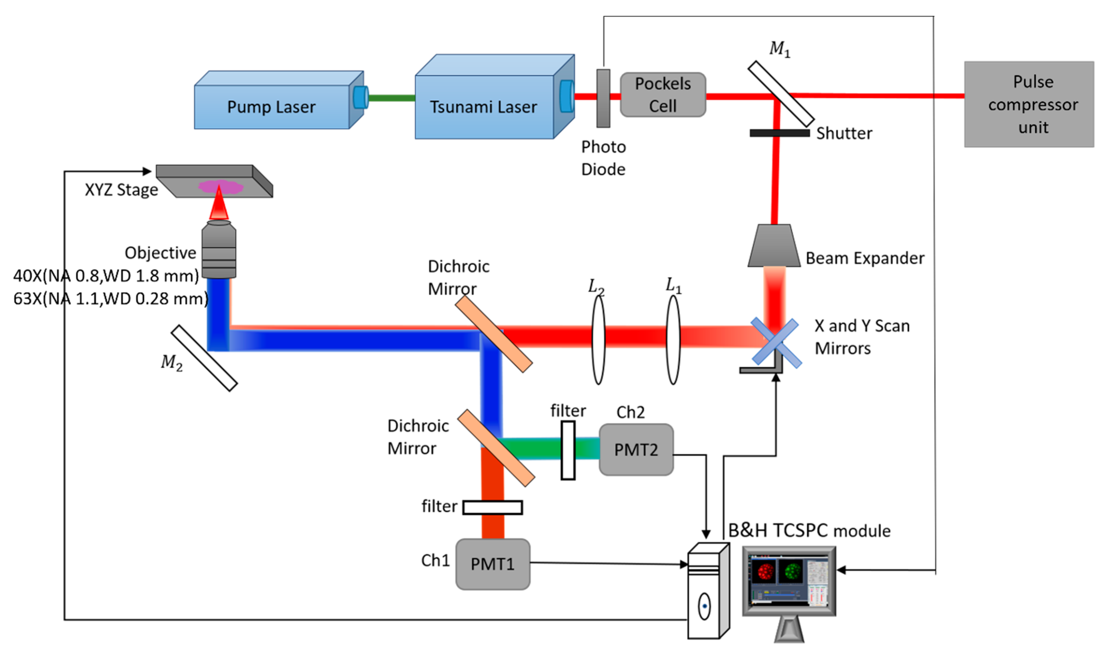
3.1. Optical Setup

An experimental MPM setup was used for the entire FCS experiments. The schematic diagram of the experimental multiphoton setup is shown in Figure 2. Two-photon excitation was achieved by a mode locked femtosecond pulsed Ti: Sapphire laser (Tsunami laser, Spectra Physics, Santa Clara, CA, USA) pumped by Millenia laser (532 nm, Spectra Physics, Santa Clara, CA, USA532 nm) and the laser intensity was modulated by a Pockels cell (350-80LA, ConOptics, Danbury, CT, USA). The excitation wavelength was set to 800 nm with an average laser power of around 20 mW. The pulse width dispersion (~100 fs) at sample plane was ascertained by an autocorrelator (CARPE, APE GmbH, Berlin, Germany) and pulse compressor (Femto control kit, APE GmbH, Berlin, Germany). Two water immersed objective lenses (40×, NA 0.8 C Achroplan NIR—working distance 1.8 mm and 63×, NA 1.2 C Apochromat—working distance 0.28 mm Carl Zeiss, Oberkochen, Germany) were employed for all measurements. The fluorescent signals were collected by two GaAsP detectors (H7422P-40 MOD, Hamamatsu Photonics, Hamamatsu, Japan), interfaced to time correlated single photon counting modules (SPC 150, Becker & Hickl GmbH, Berlin, Germany). Two spectral detection channels were enabled by using a dichroic mirror (550 nm cut off, Semrock Inc, New York, NY, USA) combined with two filters 580/150 nm and 525/50 nm (Semrock Inc, New York, NY, USA) which enabled two channels 1 (red, 550–655 nm) and 2 (blue, 417–477 nm). A sample volume of ~0.5 mL was placed in a cell dish with glass bottom (µ-Dish 35 mm, Ibidi GmbH, Gräfelfing, Germany) which was mounted on MPM stage. FCS measurements were performed by parking the laser beam at a specific location within the sample. Each measurement had the duration of 30 s and measurements were repeated 5 times to get statistical average. Autocorrelation traces were saved from each step and raw data extracted from SPCM64 software (version 9.82, Becker&Hickl GmbH, Berlin, Germany) and burst analyser (burst analyser 2, Becker&Hickl GmbH, Berlin, Germany). All FCS diagrams were plotted and analysed in MATLAB (MathWorks Inc., Natick, MA, USA) using a customized code (see Supplementary Material).

3.2. Chemicals

Solutions of Rhodamine B (Sigma Aldrich AB, Stockholm, Sweden) are prepared in MilliQ water at different concentration (10–100 nM).

3.3. FCS Data Analysis

Fluorescence autocorrelation data was obtained from SPCM64 software (version 9.82, Becker&Hickl GmbH, Berlin, Germany), and raw data were extracted from burst analyser software (burst analyser 2, Becker&Hickl, Berlin, Germany). The time tagged photon arrival data were time binned using different binning settings. The time-binned data were subject to autocorrelation by utilizing a customized algorithm, inspired by others [37], implemented in MATLAB (MathWorks Inc., Natick, MA, USA), see further Supplementary Material. The acquired autocorrelation curves were fitted using two different models. The primary model utilized in this work was based on the original model [13] as introduced in the theory section (see Equation (2)), and here referred to as G ( τ ) simple
( τ ) simple = G ( 0 ) 1 + τ τ D
In addition, according to previous literature [22] an extended model should be used for FCS in confocal setting. This model is here referred to as G ( τ ) ext   fit corresponding to:
G ( τ ) ext   fit = G ( 0 ) 1 + τ τ D 1 + a 2 ( τ τ D )
where the parameter a is introduced as a dimensional parameter defining the dimension of excitation volume.

4. Results and Validation

4.1. Effect of Numerical Aperture (NA) on FCS Measurements

It is expected that the FCS performance will depend on the choice of objective lens. In order to employ FCS in combination with imaging MPM, it would be preferable to use objective lenses with large field-of-view and long working distances but at the cost of reducing the NA. Thus, in this study the performance of two different objective lenses were investigated under similar conditions and using the same experimental system. Figure 3 shows the effect of numerical aperture on FCS measurements obtained from two different microscope objectives, 63× (NA1.2, working distance 0.28 mm) and 40× (NA 0.8, working distance 1.8 mm) for measurements of a Rhodamine B solution at 10 nM concentration. It is evident from the figure that FCS curves can be acquired using both the 63× and 40× objective lenses; however, the amplitude of the correlation function is higher for the 63× objective, i.e., G(0) = 0.6; compared to G(0) = 0.035 for the 40× objective. This is expected as a higher NA will generate a smaller excitation volume, thereby comprising less molecules giving rise to a higher G(0) value according to Equation (3) in theory section. This consequently means that the versatility for utilizing the long working distance 40× objective lens is lower as autocorrelation amplitude will approach 0 if concentration increase further.
Included in the figure, autocorrelation curves extracted directly from the SPCM64 software using so called multi-tau binning are presented (Figure 3a,d) and compared with the linear-tau algorithm with fixed binning in logarithmic (Figure 3b,e) and linear scale (Figure 3c,f). The multi-tau algorithm was found to distort the data fitting compared to using linear-tau binning. Therefore, linear-tau binning was preferred for fitting the data (see further analysis subsequent section) while multi-tau was used during acquisition for fast display and assessment of data quality.
The results obtained from the data fitting show a shift in acquired diffusion times τ D for different objective lenses. It is in the time range of 0.05 ± 0.01ms (average from 5 measurements) for 63× objective lens and 15 ± 6 ms (average from 5 measurements) for the 40× objective lens. According to the theoretical size of the 2PE volume, as described by others [2], the axial radius is 0.17 µm for the 63× objective lens (NA 1.2, λ = 800 nm) compared to 0.23 µm for the 40× lens (NA 0.8, λ = 800 nm). Through a theoretical argument (see Supplementary Material) based on previous published theory on the relation between the diffusion constant and diffusion time in the context of size of detection volume [22], the expected shift in diffusion time should be a factor 2 for the lower NA lens. However, in this case the shift is rather in the order of a factor 300. Because of this large discrepancy, the observed shift in observed diffusion time acquired for the two different objective lenses cannot simply be related to the size of focal volume and a further interpretation of this relationship will follow.

4.2. Effect of Time Binning on FCS Measurements

The impact of time binning on the processed data after autocorrelation and the acquired diffusion times after model fitting was evaluated using TCSPC raw data in form of photon arrival times obtained from measurements of solution with Rhodamine B at different concentrations (10, 20 and 40 nM) using the 63× and 40× objective lens. The acquired autocorrelated FCS data for a specific measurement (10 nM and 63× lens) are plotted for different time binning varied from 103–106 ns in Figure 4. It is evident from the figure that at shorter time binning, i.e., 103 ns, the autocorrelated data contain too much noise to be relevant, while increasing the time binning excessively (106 ns) results in loss of information and the autocorrelation function becomes hardly recognizable. Similar behavior was observed for correlation data acquired from similar solution using 40× objective lens (see further Supplementary data, Figure S1). It is clear from this evaluation that the selection of time binning is important in order to generate relevant autocorrelation data that can be subject to further data fitting. This observation agrees with the theoretical concept of FCS as presented by Elson and Madge explained as “a time interval comparable to the characteristic diffusion time is required to generate autocorrelation function” [13].
Another way of assessing the effect of time binning is to investigate the photon count per time bin. As discussed previously, the original time correlated photon count data have a binary format where “0” means no photon, and “1” is a photon counted. As photon counts are sparse, substantial binning can be performed while retaining the binary format of the data vector. This is illustrated in Figure 5 showing the photon count per time bin vector after subject to different amount of binning in the range 103–106 ns. As shown by the figure the vector is sparse and binary up to a binning of 103 ns. This also explains the lack of autocorrelation information observed for low binning in Figure 4. When increasing the binning (>5 × 10³ ns), the photon counts per time bin start to increase above one, as shown by Figure 5, and the vector is no longer binary. Increasing the binning further both elevate photon counts per time bin and noise level. This agrees with data based on concentration fluctuations should follow Poisson statistics [12]. Similar behavior was observed for correlation data acquired from similar solution using 40× objective lens (see further Supplementary data, Figure S2). Therefore, it is important to choose a binning window for which data obey this condition. From these two analyses exploring the effect of time binning, it can be concluded that the optimum time binning is around 104–105 ns for this experimental setting. This also verifies the need to validate time-binning before performing any FCS analysis using TCSPC raw data in form of photon arrival times in order to ensure relevance of data.

4.3. Effect of Concentration on FCS Measurements

Figure 6 shows the effect of concentration on the fluorescence correlation obtained from Rhodamine B solutions using the two different objective lenses 40× and 63×. As seen in the figure, the effect of increasing the concentration results in a reduction of amplitude of the autocorrelation curve. This effect was observed from the experiments performed using both objective lenses. In the case of the 63× objective lens, the G(0) value changes from 0.6 ± 0.03 (10 nM) to 0.15 ± 0.03 (40 nM). The value of G(0) change from 0.4 ± 0.005 (10 nM) to 5 × 10⁻³ ± 0.006 (40 nM) for the 40× objective lens. Since G(0) is inversely proportional to the number of particles in the detection volume and as discussed previously (see Equation (3)), this reduction in G(0) is to be expected and in accordance with the FCS theory as higher concentration corresponds to more particles in the solution.
Similar to what has been discussed in the previous section (e.g., Figure 4), the acquired diffusion time differs for the two different objective lenses; however, the effect of increasing the concentration is different. As observed from Figure 6 the acquired diffusion time is constant within the concentration range when measured using the 63× objective lens; however, when using the 40× objective, a substantially longer diffusion time (350 ± 60 ms) appears at 40 nM concentration. Furthermore, oscillations are appearing in the autocorrelated data for higher concentrations (>20 nM) and 40× objective. The physical interpretations of these oscillations and substantially longer diffusion time are unclear but likely related to the larger and less well-defined extent of the focal volume when using an objective lens with lower NA. It is clear that the 63× objective lens yields data being less sensitive to change of concentration and thereby enables a larger operational window for concentration variability when performing FCS measurements. Thus, it is evident that the choice of NA of the objective lens plays a major role in order to generate reliable FCS data. There is an unfortunate trade off and challenge when aiming for using the same objective lens for imaging and FCS acquisition. This is a significant limitation for the applicability of MPM-FCS in biomedical research studies where image acquisition and detection of location within heterogeneous samples are central requirements.

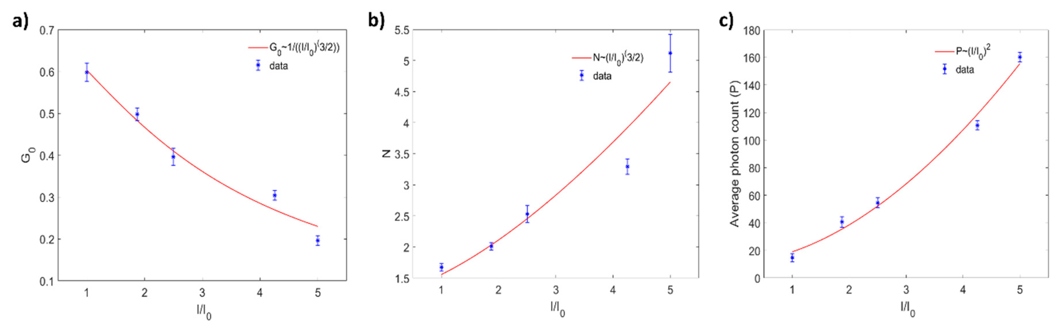
4.4. Effect of Excitation Power on FCS Measurements

Figure 7 shows the effect of excitation power on FCS measurements when the excitation power was varied between 15–50 mW and 10–30 mW for the two different objective lenses, 40× and 63× respectively, and the corresponding data and FCS model fitting are plotted. Different ranges of excitation power were applied for the objective lenses since the effective peak power inside the detection volume is expected to vary due to the difference in NA. The acquired FCS curves were found to depend on excitation intensity for both objective lenses. It is evident from the figure that excitation power will affect both parameters G(0) and diffusion time τ. In the case of the 40× objective lens, reliable FCS data were not obtained when the excitation intensities reached a lower threshold value of 15 mW and higher threshold value 50 mW. A similar behavior was observed for the 63× objective lens.
Figure 8 shows how the acquired FCS data and fitting parameters depend on the excitation intensity using the 63× objective lens. In the figure, the amplitude of autocorrelation function (G(0)), number of molecules (N) and average photon counts (P) are plotted as function of normalized excitation power (I/I0), where I0 was defined as the lowest excitation power for each objective lens. As discussed by others, ref. [29] increased excitation intensity leads to an increase in the size of the excitation volume. Therefore, the number of molecules (N) in the detection volume is expected to increase with power. Due to the inverse relation between G(0) and N, the value of G(0) decreases as excitation power increases in agreement with the experiments (Figure 8a,b). Given that the concentration in the sample is constant, N becomes proportional to the excitation volume which is expected to have an ellipsoid shape. This relationship was demonstrated by fitting the data to a curve were N~(I/I0)3/2 (Figure 8b). Subsequently, following this reasoning we can conclude that G(0) follows the relationship G(0) ~ 1/(I/I0)3/2) (Figure 8a). In Figure 8c the effect of excitation intensity on an average photon count is investigated, demonstrating a quadratic behavior, i.e., ~ (I/I0)2, as expected for two photon excitation [2]. Interestingly in these data, there are no evidence of photobleaching or excitation saturation in contrast to other reports [16,29,38]. Similar behavior was observed for the measurements using 40× objective lens (Supplementary data, Figure S3).
In addition to the above parameters, the relationship between the diffusion time and excitation intensity in the measurements was further investigated. The data from the measurements using 63× objective lens are presented in Figure 9. As shown by the figure, the values of the diffusion time were found to decrease when increasing the excitation power. Similar results were obtained using the 40× objective lens (Supplementary data, Figure S4). These results were surprising, as according to the previous theory the detected molecules are expected to diffuse through a longer distance at higher excitation intensity since the size of detection volume increases [16,39]. Previous deviations [39] from this theoretical behavior have been attributed to saturation or photobleaching effects; however, as discussed in the previous paragraph neither excitation saturation nor photobleaching was confirmed in the measurements. Instead, this deviation may be due to an alternative interpretation of the FCS measurement, as illustrated by Figure 9b. This interpretation is based on the fact that the molecules contributing to the fluorescence fluctuations are the ones at the rim of the detection volume rather than the core. The molecules confined by the detection volume will contribute to an overall increase in fluorescence signal, which agrees with the square behavior of the photon count observed in Figure 8c. Meanwhile, the molecules at the periphery of the observation volume diffuse in and out of the excitation volume and thus contribute to a faster correlation and diffusion time. At higher excitation levels, the ratio of effective surface area to size of the observation volume decreases. According to the dimensional analysis of Fick’s diffusion law, diffusion time is proportional to area when diffusion constant remains the same [40]. Thus, the diffusion time should be inversely proportional to the surface area to size ratio, i.e., the square root of the radius of the detection volume, which is related to the normalized excitation power (for further theoretical reasoning, see Supplemental Material). This inverse relationship was confirmed in the data (Figure 9a) and implies that shorter diffusion times are obtained at higher excitation intensities. This effect is most likely also contributing to the discrepancy in acquired diffusion times comparing the 40× and 63× objective lenses. As discussed previously, the confinement of detection volume using 2PE will be determined by the power distribution of excitation light in the focus. Furthermore, this effect is problematic when aiming for FCS studies in turbid media as excitation power inside the samples is expected to vary during measurements depending on the local variability of optical parameters of the sample. This spurs the need for development of protocols compensating for this effect when moving towards combination of imaging and MPM-FCS for biomedical studies of complex samples.

5. Discussion and Conclusions

The aim of this practical guideline is to clarify the conceptual principles and define experimental operating conditions in order to facilitate implementation of MPM-FCS using TCSPC. Of specific interest has been to validate and explore the potential to perform MPM-FCS using settings compliable with biomedical studies in turbid media, to allow for combination of FCS and imaging in biomedical studies. In particular, the choices of objective lens, concentration range and laser power were investigated. Furthermore, a protocol for converting raw data photon counts to autocorrelated signal was presented and the effect of binning was explored. Table 1 describes a summary of key findings along with the parameters and conditions to be considered for MPM-FCS measurements.
Two of the key parameters to be considered when performing FCS measurements using TCSPC are optimum time binning for autocorrelation and threshold range of excitation power, as also discussed by others [21]. In this study, autocorrelation curves extracted directly from the SPCM64 software using multi-tau binning and the linear-tau algorithm were compared. The analysis revealed that the data were distorted when multi-tau algorithm was used, as compared to the linear-tau binning. Instead, multi-tau was preferred for fast assessment of data during acquisition and Linear-tau algorithm was preferred for the analysis. The effect of time binning on FCS data was investigated. It was concluded from the results that it is important to find the optimum time binning for an experimental FCS which is essential to be validated before performing any FCS measurements. In this study, the optimal time binning was found to be 104–105 ns in order to allow for measurement of diffusion times in the order of 0.01–10 ms. Furthermore, the FCS analyses were performed using different excitation powers. It is clear from the measurements that the range of applied excitation power varies for objective lenses with different NA. Thus, it is necessary to validate the optimal range of excitation power and time binning for a certain experimental setup to perform FCS measurements.
One of the important aspects of extending the applicability of FCS in biomedical research is the possibility of using the same objective lens for both imaging and FCS measurements. The results demonstrated the impact of numerical aperture on FCS measurements obtained from two different microscope objectives 63× (NA1.2, working distance 0.28 mm) and 40× (NA 0.8, working distance 1.8 mm) from Rhodamine B solution at 10 nM concentration. It is evident from the results that both objective lenses had the ability to enable FCS measurements; however, the amplitude of the autocorrelation curve, G(0), acquired using the 40× (NA 0.8) objective lens was comparatively lower than 63× (NA 1.2) objective lens. This is expected as, a higher NA generate a smaller excitation volume, thus less molecules results in a higher G(0) value [9,16]. Furthermore, the concentration interval for which the measurements were possible was less for the 40× objective. Thus, the applicability of utilizing the long working distance 40× objective lens for FCS was found to be lower. An alternative approach for combining FCS and MPM would be to expand the feasibility of using high NA and short working distance objective lenses for imaging purposes. Possibly image filtering and processing could potentially aid in improving image quality using nonoptimal imaging settings. The feasibly of this approach would be possible, particularly in increasing field of view; however, it is unlikely that after processing, techniques can compensate for restrictions in working distance, which why this issue is problematic.
In addition to the limitation discussed above, the diffusion time acquired when using the two objective lenses were different. According to the theoretical relationship between the diffusion constant and diffusion time in the context of size of detection volume [11], the observed difference is larger than the expected shift. This discrepancy in the observed diffusion time acquired for the two different objective lenses cannot be explained by the size of focal volume. To date, a limited numbers of studies have investigated the relationship between focal volume optics and FCS data [39]. We further speculate that this effect is related to the results demonstrating an inverse relationship of laser power on the measured diffusion time. The study confirms an expected relationship between autocorrelation and laser power close to the equilibrium condition, i.e., at short lag times (τ → 0); however, at nonequilibrium condition, i.e., time intervals corresponding to the diffusion, the measured diffusion time was surprisingly found to be dependent on laser power. This finding can be conceptually understood in view of a dimensional analysis of Fick’s diffusion law, as the diffusion time will vary when the surface area for which the diffusion constant is defined changes given that the diffusion constant remains constant. Therefore, the measured diffusion time should be inversely proportional to the surface area to size ratio, i.e., the square root of the radius of the detection volume, which in turn is proportional to the excitation power. This inverse relationship was confirmed in the data.
To conclude, this guideline provides concepts and principles required for implementing FCS in combination with MPM. It includes crucial validation experiments that should be performed on each experimental system before undertaking FCS-MPM and that should be adapted for each specific study. Furthermore, it highlights some important limitations of the methodology, particularly when aiming at combining FCS with an experimental set up allowing for imaging MPM. Based on the novel insights on the relationship between laser power and measured diffusion times, the hope is to stimulate for the future development of protocols compensating for this effect potentially being able to work around these issues and ultimately allow MPM-FCS to become the highly useful tool in biomedical research as it is promised to be.

Supplementary Materials

The following are available online at https://www.mdpi.com/2076-3417/11/5/2122/s1, Figure S1: The effect of time binning on generating FCS curve obtained from Rhodamine B solution at a concentration of 10 nM. The data was obtained from red channel (580/150 nm) at 800 nm excitation wavelength, 25 mW excitation intensity using 40× (NA 0.8) objective lens, Figure S2: The effect of time binning on photon count rate obtained from Rhodamine B solution at concentration 10 nM. The data was obtained from red channel (580/150 nm) at 800 nm excitation wavelength, 25 mW excitation intensity using 40× (NA 0.8) objective lens, Figure S3: Plot of the (a) autocorrelation amplitude function G(0) acquired using simple data fit (G0~(I/I0)3/2) and (b) number of particles N using data fit (N~(I/I0)3/2) on autocorrelated data (time binning 10,000 ns) from experimental measurements of a Rhodamine B solution (10 nM), the 40× (NA 0.8) objective lens as a function of different laser powers, (c) average photon count as a function of excitation power. Data points in blue and red line is fitting, Figure S4: (a) Plot of the diffusion time acquired using simple data fit ( τ ~1/(I/I0)0.5 on autocorrelated data 10,000 ns) from experimental measurements of a Rhodamine B solution (10 nM), the 40× (NA 0.8) objective lens as a function of different laser powers. Data points in blue. Red lines represents fitting to two different models ( τ ~1/(I/I0)0.5 and τ ~(I/I0)) demonstrating a 1/r dependency where r is related to the size of focal volume, which will increase as laser power increases (b).

Author Contributions

Project design and planning, J.J. and M.B.E.; data acquisition, J.J.; data analysis, J.J. and M.B.E.; data and results discussion, J.J., M.B.E. and J.E.; measurements and data analysis, J.J.; supervision, M.B.E. and J.E.; writing,—original draft preparing, J.J. and M.B.E.; writing—editing and reviewing, J.J., M.B.E. and J.E.; fund acquisition and project administration, M.B.E. All authors have read and agreed to the published version of the manuscript.

Funding

Financial support was provided by Swedish Research Council (VR 2015-05002) and the Carl Trygger foundation.

Acknowledgments

The authors would like to thank Maria Smedh, Center for Cellular Imaging Core Facility, University of Gothenburg, for valuable input on the project.

Conflicts of Interest

The authors declare no conflict of interest.

References

  1. Denk, W.; Strickler, J.H.; Webb, W.W. Two-photon laser scanning fluorescence microscopy. Science 1990, 248, 73–76. [Google Scholar] [CrossRef] [Green Version]
  2. Zipfel, W.R.; Williams, R.M.; Webb, W.W. Nonlinear magic: Multiphoton microscopy in the biosciences. Nat. Biotechnol. 2003, 21, 1369–1377. [Google Scholar] [CrossRef]
  3. Sheppard, C. Scanning Confocal Microscopy. Encycl. Opt. Eng. 2003, 2525–2544. [Google Scholar] [CrossRef]
  4. Webb, R.H. Confocal optical microscopy. Rep. Prog. Phys. 1996, 59, 427–471. [Google Scholar] [CrossRef]
  5. Kirejev, V.; Guldbrand, S.; Borglin, J.; Simonsson, C.; Ericson, M.B. Multiphoton microscopy—A powerful tool in skin research and topical drug delivery science. J. Drug Deliv. Sci. Technol. 2012, 22, 250–259. [Google Scholar] [CrossRef]
  6. Konig, K. Multiphoton microscopy in life sciences. J. Microsc. 2000, 200, 83–104. [Google Scholar] [CrossRef] [PubMed]
  7. Schwille, P.; Haupts, U.; Maiti, S.; Webb, W.W. Molecular dynamics in living cells observed by fluorescence correlation spectroscopy with one- and two-photon excitation. Biophys J. 1999, 77, 2251–2265. [Google Scholar] [CrossRef] [Green Version]
  8. Haustein, E.; Schwille, P. Annual Review of Biophysics and Biomolecular Structure (ANNU REV BIOPH BIOM). Annu. Rev. Biophys. Biomol. Struct. 2007, 36, 151–169. [Google Scholar] [CrossRef] [PubMed] [Green Version]
  9. Schwille, P. Fluorescence correlation spectroscopy and its potential for intracellular applications. Cell Biochem. Biophys. 2001, 34, 383–408. [Google Scholar] [CrossRef]
  10. Schwille, P.; Heinze, K.G. Two-Photon Fluorescence Cross-Correlation Spectroscopy. ChemPhysChem 2001, 2, 269–272. [Google Scholar] [CrossRef]
  11. Magde, D.; Elson, E.L.; Webb, W.W. Fluorescence correlation spectroscopy. II. An experimental realization. Biopolymers 1974, 13, 29–61. [Google Scholar] [CrossRef]
  12. Magde, D.; Elson, E.; Webb, W.W. Thermodynamic Fluctuations in a Reacting System—Measurement by Fluorescence Correlation Spectroscopy. Phys. Rev. Lett. 1972, 29, 705–708. [Google Scholar] [CrossRef]
  13. Elson, E.L.; Magde, D. Fluorescence correlation spectroscopy. I. Conceptual basis and theory. Biopolymers 1974, 13, 1–27. [Google Scholar] [CrossRef]
  14. Rigler, R.; Mets, Ü.; Widengren, J.; Kask, P. Fluorescence correlation spectroscopy with high count rate and low background: Analysis of translational diffusion. Eur. Biophys. J. 1993, 22, 169–175. [Google Scholar] [CrossRef]
  15. Heikal, A.A.; Hess, S.T.; Baird, G.S.; Tsien, R.Y.; Webb, W.W. Molecular spectroscopy and dynamics of intrinsically fluorescent proteins: Coral red (dsRed) and yellow (Citrine). Proc. Natl. Acad. Sci. USA 2000, 97, 11996–12001. [Google Scholar] [CrossRef] [Green Version]
  16. Hess, S.T.; Webb, W.W. Focal Volume Optics and Experimental Artifacts in Confocal Fluorescence Correlation Spectroscopy. Biophys. J. 2002, 83, 2300–2317. [Google Scholar] [CrossRef] [Green Version]
  17. Wachsmuth, M.; Waldeck, W.; Langowski, J. Anomalous diffusion of fluorescent probes inside living cell investigated by spatially-resolved fluorescence correlation spectroscopy. J. Mol. Biol. 2000, 298, 677–689. [Google Scholar] [CrossRef] [Green Version]
  18. Schwille, P.; Oehlenschlager, F.; Walter, N.G. Quantitative hybridization kinetics of DNA probes to RNA in solution followed by diffusional fluorescence correlation analysis. Biochemistry 1996, 35, 10182–10193. [Google Scholar] [CrossRef]
  19. Widengren, J.; Mets, Ü.; Rigler, R. Fluorescence correlation spectroscopy of triplet states in solution: A theoretical and experimental study. J. Phys. Chem. 1995, 99, 13368–13379. [Google Scholar] [CrossRef]
  20. Schwille, P.; Korlach, J.; Webb, W.W. Fluorescence correlation spectroscopy with single-molecule sensitivity on cell and model membranes. Cytometry 1999, 36, 176–182. [Google Scholar] [CrossRef]
  21. Kim, S.A.; Heinze, K.G.; Schwille, P. Fluorescence correlation spectroscopy in living cells. Nat. Methods 2007, 4, 963–973. [Google Scholar] [CrossRef]
  22. Lakowicz, J.R. Principles of Fluorescence Spectroscopy; Springer Science+ Business Media: Berlin, Germany, 2006; pp. 1–954. [Google Scholar]
  23. Wang, Z.; Shah, J.V.; Chen, Z.; Sun, C.H.; Berns, M.W. Fluorescence correlation spectroscopy investigation of a GFP mutant-enhanced cyan fluorescent protein and its tubulin fusion in living cells with twophoton excitation. J. Biomed. Opt. 2004, 9, 395–403. [Google Scholar] [CrossRef] [PubMed]
  24. Guldbrand, S.; Kirejev, V.; Simonsson, C.; Goksör, M.; Smedh, M.; Ericson, M.B. Two-photon fluorescence correlation spectroscopy as a tool for measuring molecular diffusion within human skin. Eur. J. Pharm. Biopharm. 2013, 84, 430–436. [Google Scholar] [CrossRef] [PubMed]
  25. Benham, G.S. Chapter 6—Practical Aspects of Objective Lens Selection for Confocal and Multiphoton Digital Imaging Techniques. In Methods in Cell Biology; Matsumoto, B., Ed.; Academic Press: Cambridge, MA, USA, 2002; Volume 70, pp. 245–299. [Google Scholar]
  26. Török, P.; Kao, F. Optical Imaging and Microscopy; Springer: Berlin/Heidelberg, Germany, 2007; Volume 87. [Google Scholar] [CrossRef]
  27. Young, M.D.; Field, J.J.; Sheetz, K.E.; Bartels, R.A.; Squier, J. A pragmatic guide to multiphoton microscope design. Adv. Opt. Photonics 2015, 7, 276–378. [Google Scholar] [CrossRef] [PubMed] [Green Version]
  28. Negrean, A.; Mansvelder, H.D. Optimal lens design and use in laser-scanning microscopy. Biomed. Opt. Express 2014, 5, 1588–1609. [Google Scholar] [CrossRef] [Green Version]
  29. Becker, W.; Bergmann, A.; Haustein, E.; Petrasek, Z.; Schwille, P.; Biskup, C.; Kelbauskas, L.; Benndorf, K.; Klöcker, N.; Anhut, T.; et al. Fluorescence lifetime images and correlation spectra obtained by multidimensional time-correlated single photon counting. Microsc. Res. Tech. 2006, 69, 186–195. [Google Scholar] [CrossRef]
  30. Felekyan, S.; Kühnemuth, R.; Kudryavtsev, V.; Sandhagen, C.; Becker, W.; Seidel, C.A.M. Full correlation from picoseconds to seconds by time-resolved and time-correlated single photon detection. Rev. Sci. Instrum. 2005, 76, 1–14. [Google Scholar] [CrossRef]
  31. Becker, W. Advanced time-correlated single photon counting techniques. In Springer Series in Chemical Physics; Springer Science & Business Media: Berlin, Germany, 2005; Volume 81, pp. 1–387. [Google Scholar]
  32. Phillips, D.; Drake, R.C. Time Correlated Single-Photon Counting (Tcspc) Using Laser Excitation. Instrum. Sci. Technol. 1985, 14, 267–292. [Google Scholar] [CrossRef]
  33. Böhmer, M.; Wahl, M.; Rahn, H.-J.; Erdmann, R.; Enderlein, J. Time-resolved fluorescence correlation spectroscopy. Chem. Phys. Lett. 2002, 353, 439–445. [Google Scholar] [CrossRef]
  34. Becker, W. The bh TCSPC Handbook, 8th ed.; Becker & Hickel: Berlin, Germany, 2019; p. 968. [Google Scholar]
  35. Stock, R.S.; Ray, W.H. Interpretation of photon correlation spectroscopy data: A comparison of analysis methods. J. Polym. Sci. Polym. Phys. Ed. 1985, 23, 1393–1447. [Google Scholar] [CrossRef]
  36. James, J.; Kantere, D.; Enger, J.; Siarov, J.; Wennberg, A.-M.; Ericson, M. Report on fluorescence lifetime imaging using multiphoton laser scanning microscopy targeting sentinel lymph node diagnostics. J. Biomed. Opt. 2020, 25, 071204. [Google Scholar] [CrossRef]
  37. Laurence, T.A.; Fore, S.; Huser, T. Fast, flexible algorithm for calculating photon correlations. Opt. Lett. 2006, 31, 829–831. [Google Scholar] [CrossRef] [PubMed]
  38. Petrášek, Z.; Schwille, P. Photobleaching in Two-Photon Scanning Fluorescence Correlation Spectroscopy. ChemPhysChem 2008, 9, 147–158. [Google Scholar] [CrossRef] [PubMed]
  39. Berland, K.; Shen, G. Excitation saturation in two-photon fluorescence correlation spectroscopy. Appl. Opt. 2003, 42, 5566–5576. [Google Scholar] [CrossRef] [PubMed]
  40. Fick, A.V. On liquid diffusion. Lond. Edinb. Dublin Philos. Mag. J. Sci. 1855, 10, 30–39. [Google Scholar] [CrossRef]
Figure 1. Schematic illustrations of the fundamental principles for a fluorescence correlation spectroscopy (FCS) experiment, (a) as adopted from the original paper by Magde et al. 1974 [13], and (b) when employing a confocal microscope setting.
Applsci 11 02122 g001
Figure 2. Schematic diagram of the experimental setup enabling multiphoton laser scanning microscopy (MPM)-FCS.
Applsci 11 02122 g002
Figure 3. The effect of numerical aperture on FCS data obtained from Rhodamine B solution at 10 nM concentration acquired by using objective lenses with different numerical aperture (NA), 40× (NA 0.8) and 63× (NA 1.2). FCS data obtained from SPCM64 software produced by multi-tau algorithm (a,d), generated by customized algorithm expressed in logarithmic (b,e) and linear scale (c,f) The data was obtained from red channel (580/150 nm) at 800 nm excitation wavelength, 25 mW excitation intensity and time binned at 104 ns.
Applsci 11 02122 g003
Figure 4. The effect of time binning in the range 103–106 ns when performing autocorrelation on photon count data acquired from Rhodamine B solution at a concentration of 10 nM. The data was obtained from red channel (580/150 nm) at 800 nm excitation wavelength, 25 mW excitation intensity using 63× (NA 1.2) objective lens.
Applsci 11 02122 g004
Figure 5. The effect of time binning in the range 103–106 ns on photon count rate per time bin from data acquired from Rhodamine B solution at concentration 10 nM. The data was obtained from red channel (580/150 nm) at 800 nm excitation wavelength, 25 mW excitation intensity using 63× (NA 1.2) objective lens.
Applsci 11 02122 g005
Figure 6. The effect of concentration on FCS data obtained from Rhodamine B solution at different concentrations (10 nM, 20 nM and 40 nM) generated by different objective lenses (ac) 40× (NA 0.8) and (df) 63× (NA 1.2). Autocorrelation function data (blue) and fitted data (red) are shown. The data was obtained from red channel (580/150 nm) at 800 nm excitation wavelength, 25 mW excitation intensity.
Applsci 11 02122 g006
Figure 7. The effect of excitation power on FCS data obtained for Rhodamine B solution. Autocorrelation function data (blue) and fitted data (red) are shown. The data was obtained from red channel (580/150 nm) when excited at 800 nm wavelength using 40× (NA 0.8) and 63× (NA 1.2) objective lenses.
Applsci 11 02122 g007
Figure 8. Plot of the (a) autocorrelation amplitude function G(0) acquired using simple data fit (G(0) ~(I/I0)3/2) and (b) number of particles N using data fit (N~(I/I0)3/2) on autocorrelated data (time binning 10,000 ns) from experimental measurements of a Rhodamine B solution (10 nM), the 63× (NA 1.2) objective lens as a function of different laser powers. (c) the effect of excitation intensity on an average photon count. Data points in blue and red line is fitting.
Applsci 11 02122 g008
Figure 9. (a) Plot of the diffusion time acquired using simple data fit ( τ ~1/(I/I0)0.5 on autocorrelated data 10,000 ns) from experimental measurements of a Rhodamine B solution (10 nM), the 63× (NA 1.2) objective lens as a function of different laser powers. Data points in blue. Red lines represent fitting to two different models ( τ ~1/(I/I0)0.5 and τ ~(I/I0)) demonstrating a 1/r dependency where r is related to the size of focal volume, which will increase as laser power increases as shown in (b).
Applsci 11 02122 g009
Table 1. Summary of results describing the parameters to be considered for FCS measurements.
ParametersConditionsObservations and Recommendations
Objective lensHigh NA objective lenses (NA > 1) are preferred for FCS; however, for imaging MPM the long working distances normally restricts NA.
  • Higher NA leads to less distortions in FCS data and more reliable diffusion measurements.
  • Lower NA (NA < 1) objective lenses can be used but careful validation is required.
Concentration rangeThe concentration should preferably be in nM range for FCS, but for imaging the concentration range can vary by several orders of magnitudes.Concentration ranges needs to be validated prior to measurements:
  • Autocorrelation trace should be devoid of oscillations or distortions that may appear at higher concentration range.
  • The amplitude of the autocorrelation function (G(0)) needs to be above the threshold value.
  • The measured translational diffusion time needs to be comparable with theoretical translational diffusion time.
Excitation powerIn MPM-FCS the excitation power will determine the excitation and detection volume.
  • Look for inverse relationship of laser power on the measured diffusion time using simple model fit.
  • Based on this relationship, find the threshold range of excitation power that can be applied for certain objective lenses.
Time binningTCSPC raw data has a sparse binary data format, and time binning is required in order to perform autocorrelation.The optimal range of time binning should be validated for the specific experiments.
  • Photon count per time bin should increase above binary value
  • Photon distribution over time binning should follow Poison distribution.
Autocorrelation algorithmMulti-tau and extended data fitting models have been proposed in the literature. Here it is shown that linear-tau and simple model fitting is preferred for the data analysis.
  • Multi-tau view can be used for fast data assessment during acquisition
  • For data analysis, linear tau and simple model are preferable to enable systematic validation of parameters above.
Publisher’s Note: MDPI stays neutral with regard to jurisdictional claims in published maps and institutional affiliations.

