Shear Wave Velocity Estimation Using the Real-Time Curve Tracing Method in Ultrasound Elastography

Abstract

The estimation of shear wave velocity is very important in ultrasonic shear wave elasticity imaging (SWEI). Since the stability and accuracy of ultrasonic testing equipment have been greatly improved, in order to further improve the accuracy of shear wave velocity estimation and increase the quality of shear wave elasticity maps, we propose a novel real-time curve tracing (RTCT) technique to accurately reconstruct the motion trace of shear wave fronts. Based on the curve fitting of each frame shear wave, the propagation velocity of two-dimensional shear waves can be estimated. In this paper, shear wave velocity estimation and shear wave image reconstruction are implemented for homogeneous regions and stiff spherical inclusion regions with different elasticity, respectively. The experimental result shows that the proposed shear wave velocity estimation method based on the real-time curve tracing method has advantages in accuracy and anti-noise performance. Moreover, by eliminating artifacts of shear wave videos, the velocity map acquired can restore the shape of inclusions better. The real-time curve tracing method can provide a new idea for the estimation of shear wave velocity and elastic parameters.

1. Introduction

The elastic information of biological tissue can provide valuable references for the diagnosis of tissue function and lesions [1,2,3,4,5]. In 1998, Sarvazyan et al. proposed ultrasonic shear wave elasticity imaging technology [6]. Sandrin et al. utilized ultrafast ultrasonic imaging to catch the resulting shear wave and proposed the real-time shear wave elastic imaging algorithm in 1999 [7], which promotes the rapid development of ultrasonic elastography. There is abundant evidence that shear wave elastography (SWE) can effectively and reliably quantify the elastic characteristics of various tissues [8,9,10,11]. Ultrasonic shear wave elastography has developed rapidly because it can calculate the elastic distribution of soft tissue according to the propagation velocity of shear waves. This technology includes transient elastography (TE) [12], acoustic radiation force impulse imaging (ARFI imaging) [13,14], comb-push ultrasound shear elastography (CUSE) [15,16], supersonic shear imaging (SSI) [17,18], etc. Supersonic shear imaging is one of the most advanced shear wave elastic imaging methods, and it shows great advantages in noninvasive evaluations of liver and breast [19,20,21]. In addition, it is widely used in clinical trials [22,23], which can better reflect the elastic information of tissue.

When using the supersonic shear imaging technology, there are a large number of techniques for reconstructing the velocity image based on the mechanical properties. At present, the elastic value of tissue is characterized by estimating shear wave velocity, including the time-to-peak (TTP) method [24], the correlation-based method [25], the lateral peak (LP) method [26], the algebraic inversion method [27], Radon transform method [28,29], etc. However, the uncertainty of noise in ultrasonic motion signal limits the aforementioned methods’ application in the ultrasonic direction [26]. Based on this, McLaughlin et al. proposed a method to estimate the local shear wave velocity by obtaining the displacement information of shear waves through time signal cross-correlation in 2006 [25]. Palmeri et al. proposed the time-to-peak (TTP) method to characterize the shear wave velocity by using the time peak displacement data of the acoustic radiation force response outside the excitation region in 2008 [24]. The time-to-peak method has been successfully applied to shear wave elasticity imaging [30,31]. In order to improve the robustness of the time-to-peak method, Wang et al. introduced an application of random sample consensus (RANSAC) to estimate shear wave velocity from tissue displacement tracked by ultrasound in vivo [32]. Carrascal et al. proposed two modified shear wave velocity estimation algorithms in 2017, one of which is to search for the maximum motion in space and time, and the other of which is to apply amplitude filters to select points with a motion amplitude higher than the threshold of the shear wave group velocity estimation [26]. As this kind of peak method depends on the accurate identification of peak information, it is still necessary to improve the method of shear wave velocity estimation in the presence of noisy motion data.

We propose a real-time curve tracing (RTCT) method for shear wave trajectory, and carry out velocity estimation and two-dimensional shear wave velocity image reconstruction since the aforementioned peak method is susceptible to the local maximum when estimating the shear wave velocity. Based on the peak method, the real-time curve tracing method starts from the perspective of image processing and improves the accuracy of shear wave velocity estimation to a certain extent through connected domain processing. The accuracy of the real-time curve tracing method is proved on an ultrasound phantom by using inclusions that are softer and harder than the background material for velocity image reconstruction. At the same time, the influence of variable Gaussian noise on the accuracy of the method is studied to verify its robustness. In addition, we reproduce the velocity estimation results of two different peak measurement methods in the same phantom, and make a comparison and analysis.

2. Method and Principle

In this paper, shear waves are generated by ultrasonic radiation force. Firstly, the relationship between the energy of shear wave and the distance of the focus point is obtained by the log compressed B-mode data, that is, to search the spatial distribution of each time $i$ ($i=\left[1:i\right]$) on all $i$ time points, as shown in Equation (1).

$$S_i=\arg \left\{\max \left(u\left(x,t_i\right)\right)\right\}$$

(1)

where the displacement spatiotemporal data is given by $u\left(x,t\right)$, and the $\arg \left\{·\right\}$ operator is intended to obtain the indices for the points related to the maximum of the displacement profiles.

The position information of each point corresponding to $S_i$ is found in the frame $ith$ image $f_i\left(x,y\right)$ of the shear wave propagation video (where $\left(x,y\right)$ are the pixel coordinates, the transverse pixel spacing is 0.25 λ and the longitudinal pixel spacing is 0.5 λ, 1 λ = 0.2464 mm). Taking these points as the center, a range is determined with the standard of excitation duration, and then convolution is performed in the range with a 5 × 5 Sobel operator and $f_i\left(x,y\right)$. In other words, the position of each point corresponding to $C_i$ is taken as the center, and the edge is searched $ith$ times in a certain range. The approximate luminance difference matrices $G_x$ and $G_y$ in x and y directions are obtained, as shown in Equations (2) and (3), where $\ast$ is the convolution operation.

$$G_x=\left[\begin{array}{ccccc}1& 2& 0& -2& -1\\ 4& 8& 0& -8& -4\\ 6& 12& 0& -12& -6\\ 4& 8& 0& -8& -4\\ 1& 2& 0& -2& -1\end{array}\right]\ast f_i\left(x,y\right)$$

(2)

$$G_y=\left[\begin{array}{ccccc}-1& -4& -6& -4& -1\\ -2& -8& -12& -8& -2\\ 0& 0& 0& 0& 0\\ 2& 8& 12& 8& 2\\ 1& 4& 6& 4& 1\end{array}\right]\ast f_i\left(x,y\right)$$

(3)

Finally, the gradient magnitude M and direction θ of each pixel are calculated. The gradient amplitude and direction angle are obtained by polar coordinate transformation, which are expressed by Equations (4) and (5).

$$M\left(x,y\right)=\sqrt{G_x{\left(x,y\right)}^2+G_y{\left(x,y\right)}^2}$$

(4)

$$\theta \left(x,y\right)=\arctan \left(\frac{G_x\left(x,y\right)}{G_y\left(x,y\right)}\right)$$

(5)

where $M\left(x,y\right)$ and $\theta \left(x,y\right)$ reflect the intensity and the direction of the image edge, respectively.

In order to determine the edge information more accurately, we keep the maximum value of the local gradient and suppress its non-maximum value. The gradient intensity of the current pixel $M\left(x,y\right)$ is compared with the gradient intensity of four pixels along its positive and negative gradient directions. If the gradient intensity of the current pixel is higher than that of the other four pixels, the pixel is retained as an edge point. After that, we need to select and connect the edge points, and the specific operation is as follows: (1) selecting the appropriate threshold T, (2) marking the edge points whose gradient amplitudes are greater than T, (3) connecting the marked edge points to form a closed curve.

After $i$ times of searching, the edge information of each search is determined, and it is connected to form a closed curve. Then, the intersection of the closed curves containing any point of $C_i$ in the $i$ times search is taken as a connected domain. Meanwhile, to eliminate the artifacts of shear wave propagation, this paper includes a directional filter matrix. A directional filter with a minimum circumscribed rectangle is designed for the connected domain of the shear wave image, and the data outside the directional filter are set to 0. Next, Gaussian filtering is applied to the shear wave image $h_i\left(x,y\right)$ after this processing, and the filtered image $p_i\left(x,y\right)$ is obtained, as shown in Equation (6).

$$\begin{array}{l}{p}_i\left(x,y\right)=K\left(x,y,\sigma \right)\ast h_i\left(x,y\right)\\ =\left(\frac{1}{2\pi {\sigma }^2}{e}^{-\frac{x^2+y^2}{2{\sigma }^2}}\right)\ast h_i\left(x,y\right)\end{array}$$

(6)

where $K\left(x,y,\sigma \right)$ is the two-dimensional Gaussian kernel function, $\sigma$ is the standard deviation and $\ast$ denotes convolution operation.

Finally, the connected domain of the directional filter in image $p_i\left(x,y\right)$ is regarded as the shear wave front, and the center points in each transverse direction in the connected domain of the shear wave front are connected into a smooth curve to complete the real-time curve tracing of the shear wave front.

From the perspective of image processing, the real-time curve tracing method utilizes a curve to fit the discontinuous shear wave with a certain width, which can realize the real-time visualization of shear wave propagation. Based on the above principle, we reconstruct the shear wave velocity image by using the real-time tracing curve of shear wave propagation. For the selected region of interest (ROI), the shear wave velocity $V\left(x,y\right)$ of the pixel point $\left(x,y\right)$ is given by Equation (7).

$$V\left(x,y\right)=\frac{\Delta x}{\Delta t}$$

(7)

where $\Delta x$ is the displacement of the shear wave tracing curve relative to the previous frame, and $\Delta t$ is the interval time between each frame of the shear wave.

Equation (7) can be used to calculate the propagation velocity of the shear wave in the region of interest at each pixel, so as to reconstruct the shear wave velocity image. Certainly, interpolation and filtering algorithms can make the speed reconstruction image have better resolution and contrast. Then, the reconstructed shear wave velocity image is transformed into a two-dimensional ultrasonic elastic image by Equation (8).

$$E=3\rho c^2$$

(8)

where E is Young’s modulus, ρ is the density of the tissue and c is the shear wave propagation velocity.

3. Phantom Experiments

3.1. Experimental Environment

The excitation and acquisition of the shear wave are realized by the Verasonics ultrasonic experimental system (America), and its model is Vantage 256. The L11-4V ultrasonic linear array probe is used in the experiment, and its center frequency is 6.25 MHz. We use an ultrafast plane wave imaging technique to image the propagation of the resulting transient plane shear waves. Other parameters of the system are shown in Table 1.

Table 1. Multi-focus excitation acquisition parameters.

Acquisition Parameter	Title 3
Wavelength (λ)	0.2464 mm
Acoustic velocity (m/s)	1540
Excitation frequency (Hz)	6.25 × 106
Excitation duration (cycles)	1200
Number of array elements used in acoustic radiation force generation	32
Four focal points using supersonic shear imaging technology (λ)	20,40,60,80
Transverse range of region of interest (λ)	−20~80
Transverse resolution of beamforming (λ)	0.25
Longitudinal range of region of interest (λ)	15~95
Longitudinal resolution of beamforming (λ)	0.5
Excitation voltage (V)	50
Channel data sampling frequency (Hz)	25 × 106
Each frame acquisition interval (us)	100
Capture shear wave frame number	70

Four experiments are conducted in a 040GSE ultrasound phantom with a background elasticity of 30 kPa by the supersonic shear imaging method. The selected experimental areas are shown in Figure 1, in which the red rectangle represents the region of interest for each experiment, and the dotted box in the red rectangle is the range for velocity estimation. In other words, the dotted box is considered to be the main propagation area of the right shear wave in each group of experiments, which is also our targeted imaging area.

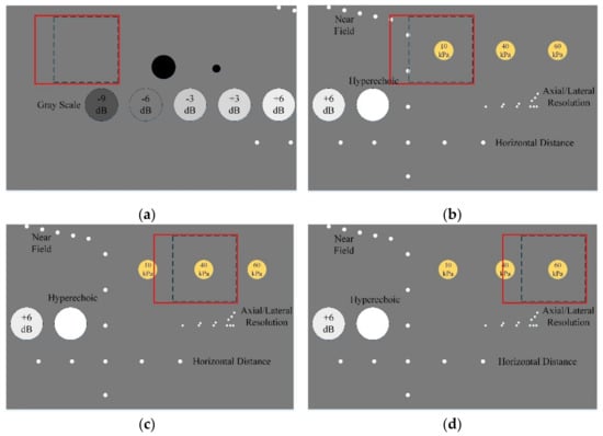
Figure 1. The selected experimental area in 040GSE ultrasound phantom. (a) The selected experimental area of homogeneous region. (b) The selected experimental area containing a 10 kPa inclusion. (c) The selected experimental area containing a 40 kPa inclusion. (d) The selected experimental area containing a 60 kPa inclusion.

In Figure 1a, a larger solid black circle and a smaller solid black circle on the right side of the region of interest represent the anechoic stepped cylinders. The circles with different decibels on the lower side of the region of interest represent grayscale target groups, ranging from −9 dB to +6 dB. In the region of interest of Figure 1b–d, there are inclusions with a diameter of 6 mm, which are different from the background elasticity, and their elasticity is 10 kPa, 40 kPa and 60 kPa, respectively. In these figures, the small white dots far smaller than the size of the inclusions are the target points, and the white circle without markings is a hyperechoic region of the same size as the other grayscale target groups.

3.2. Shear Wave Velocity Estimation

In this paper, the real-time curve tracing is performed for the 10th frame image of shear wave propagation in the targeted imaging area of Figure 1a. Figure 2a shows the original propagation trajectory of the shear wave. The shear wave front is obtained by the directional filter matrix, and then the central point of each transverse shear wave front is connected, as shown with the red curve of Figure 2b. Since the shear wave propagates in a homogeneous region, the tracing curve is close to a straight line with an inclination angle. Then, we do the same operation for the 30th frame image of shear wave propagation in the targeted imaging area of Figure 1d. Similarly, Figure 2c shows the original propagation trajectory of the shear wave, and the tracing curve is shown with the red curve of Figure 2d. Owing to the deformation of the shear wave front at the inclusion, the tracing curve protrudes to the right, which is consistent with the expected result. Because the shear wave front cannot cover the whole longitudinal range, we set two transverse lines at the head and tail of the shear wave front.

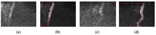
Figure 2. Experimental results of real-time curve tracing. (a) The 10th frame image of shear wave propagation in homogeneous region. (b) Tracing curve of (a). (c) The 30th frame image of shear wave propagation in the region containing a 60 kPa inclusion. (d) Tracing curve of (c).

Generally, the isotropic homogeneous region is used to analyze and evaluate the estimation method of shear wave velocity [33]. For the homogeneous region, the shear wave velocity can be quickly estimated by taking the lateral moving distance of several tracing curves in the same transverse direction as the shear wave displacement.

With the real-time curve tracing method, the tracing curves of each frame of the high-frame rate shear wave propagation in the homogeneous region of Figure 1a can be obtained. Figure 3 lists the six tracing curves that are initially frame 4 and frame interval 5. Directly perceived from Figure 3, the shear wave tracing curve is an approximately inclined straight line, and the interval of each curve is roughly equal. On the one hand, these characteristics reflect the Mach cone shape of shear wave and, on the other hand, they reflect that the shear wave propagates at a uniform speed, which indicates that the targeted area is homogeneous. Since the longitudinal range of the data that can be used to calculate the wave velocity is different in each frame, the common part of these frames is selected to estimate the shear wave velocity (about 25 λ to 85 λ). A to F are the intersections of the tracing curves of the 4th, 9th, 14th, 19th, 24th and 29th frames at a depth of 55 λ, respectively. By performing linear regression processing on the ordinates of these six intersections, the propagation velocity of the shear wave in the specified transverse direction can be estimated. Of course, one can choose the intersection point of any number of frames at a certain transverse position for linear regression to estimate the propagation velocity of the shear wave in the homogeneous region. The estimation error decreases with the increase in frame number.

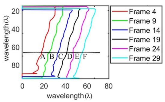
Figure 3. Tracing curves of shear wave propagation trajectories with different frames.

To verify and compare the performance of the proposed method, the time-to-peak and the lateral peak method are used to estimate the shear wave velocity in the homogeneous region under the same conditions, taking a homogeneous region with a Young’s modulus of 30 kPa as an example. The implementation processes of the time-to-peak method and the lateral peak method are shown in Figure 4. The time-to-peak method finds out the maximum time of shear wave displacement in each transverse position. The curves in Figure 4a describe the relationship between the energy of the shear wave and the time at different displacements (these data were normalized). Therefore, the shear wave velocity can be estimated from the known displacement and the time to peak, as shown in Figure 4c. The lateral peak method is used to select the information of the shear wave energy peak point to process. As shown in Figure 4b, the curves describe the relationship between the shear wave energy and distance away from the focus point at different times (these data were normalized). In that way, the velocity of the shear wave in a certain period of time can be estimated by the known time interval and the peak displacement, as shown in Figure 4d.

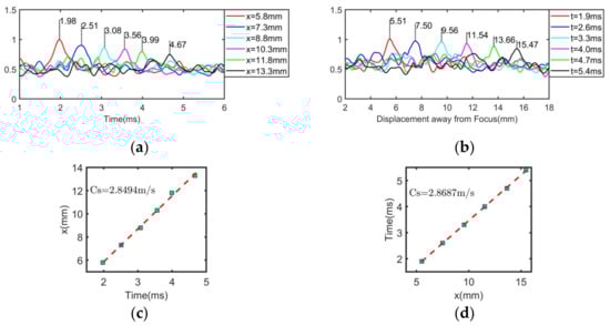
Figure 4. Experimental result of shear wave velocity estimation with the time-to-peak and the lateral peak method. (a) Velocity estimation using time-to-peak method. (b) Velocity estimation using lateral peak method. (c) Linear regression results of time-to-peak method. (d) Linear regression results of lateral peak method. Subfigures (a,b) are normalized.

3.3. Image Reconstruction of Shear Wave Velocity

3.3.1. Homogeneous Region

According to the real-time curve tracing method proposed in this paper, the experimental data of a high-frame rate shear wave propagation video can be obtained in the homogeneous region of the 040GSE ultrasound phantom shown in Figure 1a, with which the shear wave velocity image reconstruction is realized. The B-ultrasound image of the homogeneous area is shown in Figure 5a. In the B-ultrasound image, the thick red line at the top corresponds to the position of the probe, the white rectangle is the selected region of interest and the four red cross marks in the longitudinal direction correspond to the focus coordinates in Table 1. The real-time curve tracing method is utilized to reconstruct the shear wave velocity image of the selected region of interest in the homogeneous region of the 040GSE ultrasound phantom. In order to facilitate the presentation of the reconstruction effect, the results in Figure 5b are selected for subsequent detailed analysis, with a transverse range of 20 λ to 60 λ and a longitudinal range of 30 λ to 80 λ.

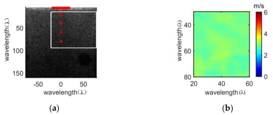
Figure 5. Velocity image reconstruction in the homogeneous region with the real-time curve tracing method. (a) The B-ultrasound image of region of interest. (b) The velocity imaging.

3.3.2. Stiff Spherical Inclusion Regions with Varying Elastic Values

In this subsection, the shear wave velocity images of the region of interest containing a stiff spherical inclusion in Figure 1b–d are reconstructed, of which the B-ultrasound images are shown in Figure 6(a-1,a-2,a-3), respectively. The elasticity of the inclusions is 10 kPa, 40 kPa and 60 kPa, and the background elasticity is 30 kPa. When reconstructing the shear wave velocity image of the stiff spherical inclusion regions, the image processing is the same as that of the homogeneous area. Two targeted regions are intercepted for subsequent analysis, as shown in Figure 6(b-1,b-2,b-3). The background is selected as the black rectangle area with a transverse range of 30 λ to 50 λ and a longitudinal range of 25 λ to 35 λ. The inclusion is selected as the black circular area with a diameter of 24 λ, about 6 mm.

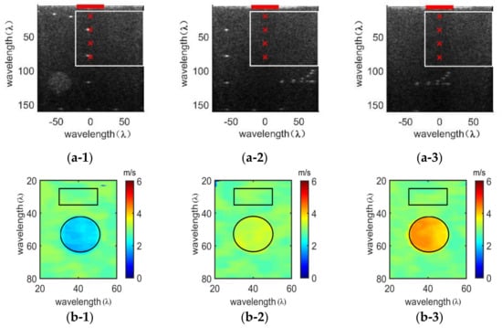
Figure 6. Velocity image reconstruction of the stiff spherical inclusion with the real-time curve tracing method. (a) The B-ultrasound image of region of interest. (b) The velocity imaging. (a-1) The B-ultrasound image of the region containing a stiff spherical inclusion of 10 kPa. (a-2) The B-ultrasound image of the region containing a stiff spherical inclusion of 40 kPa. (a-3) The B-ultrasound image of the region containing a stiff spherical inclusion of 60 kPa. (b-1) The velocity image of the region containing a stiff spherical inclusion of 10 kPa. (b-2) The velocity image of the region containing a stiff spherical inclusion of 40 kPa. (b-3) The velocity image of the region containing a stiff spherical inclusion of 60 kPa.

3.4. Noise Adaptability

In theory, even under different noises, the motion state of a shear wave can be accurately characterized as long as the propagation trajectory of the shear wave can be identified. In order to further analyze the noise adaptability of the real-time curve tracing method, the shear wave propagation images are processed under different noises. Four frame tracing curves with an initial frame number of 10 and frame interval of 5 are selected as raw reference data to conduct two sets of experiments. In the first experiment, these raw reference data are contaminated with zero-mean Gaussian noise, of which the standard deviation (STD) is set to 0.1, 0.2 and 0.3. In the second set of experiments, the mean value of Gaussian noise added in the raw reference data is set to 0.05, 0.1 and 0.2, and the standard deviation is 0.1. The results of the above two sets of experiments are given in in Figure 7 and Figure 8, respectively.

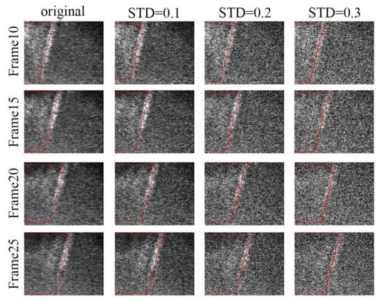
Figure 7. Gaussian noise experiment with equal noise mean.

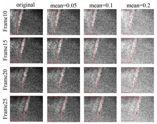
Figure 8. Gaussian noise experiment with equal noise standard deviation.

4. Results

4.1. Evaluation of Shear Wave Velocity

In the experiment, the real-time curve tracing method is used to estimate the transverse propagation velocity of a shear wave in the selected homogeneous region, and the results are compared with those of the time-to-peak method and the lateral peak method. According to the experimental method in Section 3.2, these three methods selected 50 points in each transverse direction for data analysis to ensure consistency and fairness. In the longitudinal range of 25 λ to 85 λ, 61 groups of transverse data were selected at intervals of 1 λ. With regard to the real-time curve tracing method, linear regression is performed on each group of transverse data, as shown in Figure 3, and then the average value of the 61 groups is obtained as the shear wave velocity in the homogeneous region. With regard to the time-to-peak method and the lateral peak method, the shear wave velocity is calculated by the peak information of the shear wave. The confidence interval is 95%, and the results are shown in Figure 9. The expression of velocity is average ± standard deviation, and the results are shown in Table 2. In this paper, the calculation formula of relative error X_R is shown in Equation (9).

$$X_R=\frac{V_T-V_E}{T_T}\times 100\%$$

(9)

where V_T is the theoretical velocity and V_E is the estimated velocity.

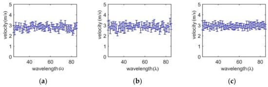
Figure 9. Velocity estimation in homogeneous region. (a) The time-to-peak method. (b) The lateral peak method. (c) The real-time curve tracing method.

Table 2. Comparison of shear wave velocity estimation.

Background Elasticity (kPa)	Theoretical Velocity (m/s)	Estimated Method	Estimated Velocity (m/s)	Relative Error (%)
30	3.1623	The time-to-peak method	2.8078 ± 0.1944	11.21%
		The lateral peak method	2.8622 ± 0.2114	9.49%
		The real-time curve tracing method	2.9382 ± 0.1221	7.09%

4.2. Result of Velocity Reconstruction Image

In the homogeneous region, the experimental data of velocity image reconstruction in the intercepted homogeneous area shown in Figure 5b are quantitatively analyzed. The estimated velocity of the shear wave in the homogeneous area with the real-time curve tracing method is 2.9026 m/s, the standard deviation is 0.1032 m/s and the relative error is 8.21%.

In the stiff spherical inclusion regions with varying elastic values, the experimental data of velocity image reconstruction in the black rectangle intercepted area and the background area shown in Figure 6b are quantitatively analyzed. The comparison results are shown in Table 3.

Table 3. Comparison of shear wave velocity estimation. Analysis of velocity image reconstruction in the intercepted area and the background area with the real-time curve tracing method.

Modulus of Elasticity (kPa)		Theoretical Velocity (m/s)	Estimated Velocity (m/s)	Relative Error (%)
1	Inclusion: 10	1.8257	1.9544 ± 0.3914	7.05%
	Background: 30	3.1623	2.9179 ± 0.2236	7.73%
2	Inclusion: 40	3.6514	3.3501 ± 0.5583	8.25%
	Background: 30	3.1623	2.9797 ± 0.2179	5.77%
3	Inclusion: 60	4.4721	4.1692 ± 0.6952	6.77%
	Background: 30	3.1623	2.9754 ± 0.2328	5.91%

When the elasticity of inclusion is 40 kPa, 10 kPa and 60 kPa, the estimated relative errors are 8.25%, 7.05% and 6.77%, respectively, which means that the relative error of estimation velocity gradually decreases with the increase in the elastic difference between inclusion and background.

4.3. Noise Adaptability Results

From Figure 7 and Figure 8, we can see that even in the case of noise, the real-time curve tracing method can still express the shear wave trajectory accurately. Since the longitudinal range of the shear wave tracing curve has changed after adding noise, this paper only selects and analyzes the common longitudinal range of four tracing curves, namely, 25 λ to 85 λ. Hereon, the real-time curve tracing method is used to estimate the shear wave velocity under the condition of no artificial noise or different noises, and the standard deviation and relative error are compared. The results are shown in Figure 10, Figure 11 and Table 4, and the theoretical shear wave velocity is 3.1623 m/s.

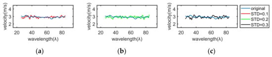
Figure 10. Shear wave velocity estimation with different standard deviation noise. The standard deviation is (a) 0.1, (b) 0.2, (c) 0.3.

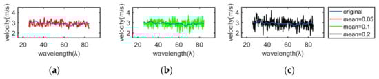
Figure 11. Shear wave velocity estimation with different mean noise. The mean is (a) 0.05, (b) 0.1, (c) 0.2.

Table 4. Estimated shear wave velocity after adding noise.

Noise Level		Estimated Velocity (m/s)	Relative Error (%)
original		2.9193 ± 0.0930	7.68%
mean = 0	STD = 0.10	2.9185 ± 0.1021	7.71%
	STD = 0.20	2.9167 ± 0.1119	7.77%
	STD = 0.30	2.9106 ± 0.1332	7.96%
STD = 0.1	Mean = 0.05	2.9111 ± 0.2110	7.94%
	Mean = 0.10	2.9069 ± 0.3181	8.08%
	Mean = 0.20	2.9033 ± 0.3938	8.19%

The results in Figure 7 and Figure 8 state clearly that the change of the Gaussian noise standard deviation will affect the blur degree of the image, and the change of the mean value will affect the brightness and darkness of the image. Compared with the blur degree of the shear wave image, the brightness and darkness of the shear wave image can affect the shear wave velocity estimation more. It can be seen in Figure 10 and Figure 11 and Table 4 that the mean value of Gaussian noise has a great influence on the shear wave velocity, which makes the standard deviation of the estimated velocity larger. Therefore, it is necessary to avoid the change of shear wave image brightness and darkness in the estimation of shear wave velocity.

5. Discussion

In the homogeneous region with an elastic modulus of 30 kPa, the estimated velocity, the standard deviation and the relative error with the time-to-peak method are 2.8078 m/s, 0.1944 m/s and 11.21%, respectively. The corresponding estimated values of the lateral peak method are 2.8622 m/s, 0.2114 m/s and 9.49%. However, the estimated velocity, the standard deviation and the relative error with the real-time curve tracing method are 2.9382 m/s, 0.1221 m/s and 7.09%, respectively. Evidently, compared to the time-to-peak method and the lateral peak method, the real-time curve tracing method improves the accuracy while estimating the shear wave velocity in the homogeneous area, which is due to the improved frame rate stability of hardware devices. The main factor affecting the accuracy of the real-time curve tracing method is the stability of the frame rate. If the frame rate stability is evaluated and modified, the accuracy of shear wave velocity estimation will be further improved. The experimental results show that the real-time curve tracing method can provide new ideas for the evaluation of shear wave velocity and elastic parameters.

It can be concluded from the experimental results of the homogeneous region of the 040GSE ultrasound phantom that the real-time curve tracing method has more advantages in image reconstruction of shear wave velocity because of its high accuracy in two-dimensional shear wave velocity estimation. In the results obtained by using the stiff spherical inclusion regions, the results fully illustrate that for the stiff spherical inclusion regions, regardless of the elasticity and location of inclusions, the shear wave velocity image can be reconstructed by using the real-time curve tracing method. The above experimental results verify the feasibility of the real-time curve tracing method for shear wave velocity image reconstruction in the stiff spherical inclusion regions.

In the noise experiment, the experimental results show that the influence of Gaussian noise on velocity estimation is small, which indicates that this method has strong noise adaptability. Since the time-to-peak method and the lateral peak method use peak data to calculate shear wave velocity, and peak value is easily affected by noise, the real-time curve tracing method has better anti-noise performance than the time-to-peak method and the lateral peak method.

In recent years, most methods are based on time domain data to estimate shear wave velocity. These methods estimate shear wave velocity by the characteristics of shear wave motion [34,35]. Among them, when the time signal cross-correlation is used to calculate the shear wave velocity [36], the size of the window will affect the measurement results of shear wave velocity. However, the proposed real-time curve tracing method avoids the influence of window size on shear wave estimation velocity by image processing technology.

At present, there are some methods to estimate shear wave velocity using frequency domain data, which are common methods proposed in recent years [37,38,39]. Most of these estimation methods have limited spatial range in the transverse and longitudinal directions. In order to change this defect, many research teams have extended these methods, such as making them generate images of phase velocity or viscoelastic characteristics [40,41]. In 2018, Kijanka and Urban proposed local phase velocity imaging to create phase velocity images at different frequencies in homogeneous and heterogeneous media using Fourier decomposition and moving windows [38]. One of the limitations of the local phase velocity imaging method is that the results may be corrupted by outliers or motion records with high noise content. However, the real-time curve tracing method can avoid outliers in image filtering.

6. Conclusions

In this paper, we present a new real-time curve tracing method to estimate the shear wave velocity. Quantitative velocity images have been achieved, particularly in the homogeneous region and in the stiff spherical inclusion regions. Compared with the traditional time-to-peak method and lateral peak method, the relative error and standard deviation of the real-time curve tracing method for velocity estimation in a homogeneous area are smaller. At the same time, the proposed method can reconstruct the shear wave velocity image more accurately. In the experiment of changing the standard deviation and mean value of Gaussian noise, the proposed method shows some robustness. The experimental results and analyses show that the real-time curve tracing method can trace the shear wave propagation in real time, and outperforms other methods in terms of the estimation accuracy. Therefore, the velocity image reconstruction and elasticity map inversion based on the real-time curve tracing method can provide more accurate and important elastic information for tissue characteristics.

References

- Amzar, D.; Cotoi, L.; Sporea, I.; Timar, B.; Schiller, O.; Schiller, A.; Borlea, A.; Pop, N.G.; Stoian, D. Shear Wave Elastography in Patients with Primary and Secondary Hyperparathyroidism. J. Clin. Med. 2021, 10, 697. [Google Scholar] [CrossRef]
- Bamber, J.; Cosgrove, D.; Dietrich, C.F. EFSUMB guidelines and recommendations on the clinical use of ultrasound elastography. Part 1: Basic principles and technology. Ultraschall Med. 2013, 34, 169–184. [Google Scholar] [CrossRef]
- Pieczewska, B.; Glińska-Suchocka, K.; Niżański, W.; Dzięcioł, M. Decreased Size of Mammary Tumors Caused by Preoperative Treatment with Aglepristone in Female Domestic Dogs (Canis familiaris) Do Not Influence the Density of the Benign Neoplastic Tissue Measured Using Shear Wave Elastography Technique. Animals 2021, 11, 527. [Google Scholar] [CrossRef]
- Yamakoshi, Y.; Sato, J.; Sato, T. Ultrasonic imaging of internal vibration of soft tissue under forced vibration. IEEE Trans. Ultrason. Ferroelect. Freq. Control. 1990, 37, 45–53. [Google Scholar] [CrossRef]
- Cepeha, C.M.; Paul, C.; Borlea, A.; Fofiu, R.; Borcan, F.; Dehelean, C.A.; Ivan, V.; Stoian, D. Shear-Wave Elastography—Diagnostic Value in Children with Chronic Autoimmune Thyroiditis. Diagnostics 2021, 11, 248. [Google Scholar] [CrossRef]
- Sarvazyan, A.P.; Rudenko, O.V.; Swanson, S.D. Shear Wave Elasticity Imaging: A new ultrasonic technology of medical diagnostics. Ultrasound Med. Biol. 1998, 24, 1419–1435. [Google Scholar] [CrossRef]
- Sandrin, L.; Catheline, S.; Tanter, M.; Hennequin, X.; Fink, M. Time-resolved pulsed elastography with ultrafast ultrasonic imaging. Ultrason. Imaging 1999, 21, 259–272. [Google Scholar] [CrossRef]
- Zhang, Z.J.; Ng, G.Y.F.; Fu, S.N. Effects of habitual loading on patellar tendon mechanical and morphological properties in basketball and volleyball players. Eur. J. Appl. Physiol. 2015, 115, 2263–2269. [Google Scholar] [CrossRef]
- Kot, B.C.W.; Zhang, Z.J.; Lee, A.W.C. Elastic Modulus of Muscle and Tendon with Shear Wave Ultrasound Elastography: Variations with Different Technical Settings. PLoS ONE 2012, 7, e44348. [Google Scholar] [CrossRef]
- Maïsetti, O.; Hug, F.; Bouillard, K. Characterization of passive elastic properties of the human medial gastrocnemius muscle belly using supersonic shear imaging. J. Biomech. 2012, 45, 978–984. [Google Scholar] [CrossRef]
- Lacourpaille, L.; Hug, F.; Bouillard, K. Supersonic shear imaging provides a reliable measurement of resting muscle shear elastic modulus. Physiol. Meas. 2012, 33, N19. [Google Scholar] [CrossRef]
- Sandrin, L.; Fourquet, B.; Hasquenoph, J.M. Transient elastography: A new noninvasive method for assessment of hepatic fibrosis. Ultrasound Med. Biol. 2003, 29, 1705–1713. [Google Scholar] [CrossRef]
- Nightingale, K.; McAleavey, S.; Trahey, G. Shear-wave generation using acoustic radiation force: In vivo and ex vivo results. Ultrasound Med. Biol. 2003, 29, 1715–1723. [Google Scholar] [CrossRef]
- Nightingale, K.; Soo, M.S.; Nightingale, R. Acoustic radiation force impulse imaging: In vivo demonstration of clinical feasibility. Ultrasound Med. Biol. 2002, 28, 227–235. [Google Scholar] [CrossRef]
- Song, P.; Zhao, H.; Manduca, A. Comb-push ultrasound shear elastography (CUSE): A novel method for two-dimensional shear elasticity imaging of soft tissues. IEEE Trans. Med. Imaging 2012, 31, 1821–1832. [Google Scholar] [CrossRef]
- Song, P.; Urban, M.W.; Manduca, A. Comb-push ultrasound shear elastography (CUSE) with various ultrasound push beams. IEEE Trans. Med. Imaging 2013, 32, 1435–1447. [Google Scholar] [CrossRef] [PubMed]
- Bercoff, J.; Tanter, M.; Fink, M. Supersonic shear imaging: A new technique for soft tissue elasticity mapping. IEEE Trans. Ultrason. Ferroelect. Freq. Contr. 2004, 51, 396–409. [Google Scholar] [CrossRef]
- Tanter, M.; Bercoff, J.; Athanasiou, A. Quantitative assessment of breast lesion viscoelasticity: Initial clinical results using supersonic shear imaging. Ultrasound Med. Biol. 2008, 34, 1373–1386. [Google Scholar] [CrossRef]
- Evans, A. Breast Shear Wave Elastography in Clinical Practice. 2019 IEEE International Ultrasonics Symposium (IUS), Glasgow, UK, 6–9 October 2019; pp. 119–121. [Google Scholar]
- Bavu, E. Noninvasive in vivo liver fibrosis evaluation using supersonic shear imaging: A clinical study on 113 hepatitis C virus patients. Ultrasound Med. Biol. 2011, 37, 1361–1373. [Google Scholar] [CrossRef] [PubMed]
- Gheonea, D.I. Real-time sono-elastography in the diagnosis of diffuse liver diseases. World J. Gastroenterol. 2010, 16, 1720–1726. [Google Scholar] [CrossRef]
- Berg, W.A.; Cosgrove, D.O.; Doré, C.J. Shear-wave elastography improves the specificity of breast us: The BE1 multinational study of 939 masses. Radiology 2012, 262, 435–449. [Google Scholar] [CrossRef]
- Zhou, J.; Zhan, W.; Chang, C. Breast lesions: Evaluation with shear wave elastography, with special emphasis on the ‘stiff rim’ sign. Radiology 2014, 272, 63–72. [Google Scholar] [CrossRef]
- Palmeri, M.L.; Wang, M.H.; Dahl, J.J.; Frinkley, K.D.; Nightingale, K.R. Quantifying hepatic shear modulus in vivo using acoustic radiation force. Ultrasound Med. Biol. 2008, 34, 546–558. [Google Scholar] [CrossRef]
- McLaughlin, J.; Renzi, D. Shear wave speed recovery in transient elastography and supersonic imaging using propagating fronts. Inverse Probl. 2006, 22, 681. [Google Scholar] [CrossRef]
- Carrascal, C.A.; Chen, S.; Manduca, A.; Greenleaf, J.F.; Urban, M.W. Improved Shear Wave Group Velocity Estimation Method Based on Spatiotemporal Peak and Thresholding Motion Search. IEEE Trans. Ultrason. Ferroelect. Freq. Contr. 2017, 64, 660–668. [Google Scholar] [CrossRef]
- Oliphant, T.E.; Manduca, A.; Ehman, R.L.; Greenleaf, J.F. Complex-valued stiffness reconstruction for magnetic resonance elastography by algebraic inversion of the differential equation. Mag. Reson. Med. 2001, 45, 299–310. [Google Scholar] [CrossRef]
- Urban, M.W.; Greenleaf, J.F. Use of the radon transform for estimation of shear wave speed. J. Acoust. Soc. Am. 2012, 132, 1982. [Google Scholar] [CrossRef]
- Rouze, N.C.; Wang, M.H.; Palmeri, M.L.; Nightingale, K.R. Robust estimation of time-of-flight shear wave speed using a radon sum transformation. IEEE Trans. Ultrason. Ferroelect. Freq. Contr. 2010, 57, 2662–2670. [Google Scholar] [CrossRef]
- Chen, S.; William, W.; Callstrom, M.R. Assessment of liver viscoelasticity by using shear waves induced by ultrasound radiation force. Radiology 2013, 266, 940–947. [Google Scholar] [CrossRef]
- Braticevici, C.F.; Andronescu, D.; Usvat, R. Acoustic radiation force imaging sonoelastography for noninvasive staging of liver fibrosis. World J. Gastroenterol. 2009, 15, 5525–5532. [Google Scholar] [CrossRef]
- Wang, M.H.; Palmeri, M.L.; Rotemberg, V.M.; Rouze, N.C.; Nightingale, K.R. Improving the robustness of time-of-flight based shear wave speed reconstruction methods using RANSAC in human liver in vivo. Ultrasound Med. Biol. 2010, 36, 802–813. [Google Scholar] [CrossRef]
- Song, P.; Manduca, A.; Zhao, H. Fast Shear Compounding Using Robust Two-dimensional Shear Wave Speed Calculation and Multi-directional Filtering. Ultrasound Med. Biol. 2014, 40, 1343–1355. [Google Scholar] [CrossRef] [PubMed]
- Rifat, A.; Gerber, S.A.; Mcaleavey, S.A. Plane wave imaging improves single track location shear wave elasticity imaging. IEEE Trans. Ultrason. Ferroelect. Freq. Contr. 2018, 65, 1402–1414. [Google Scholar]
- Racedo, J.; Urban, M.W. Evaluation of Reconstruction Parameters for 2-D Comb-Push Ultrasound Shear Wave Elastography. IEEE Trans. Ultrason. Ferroelect. Freq. Contr. 2019, 66, 254–263. [Google Scholar] [CrossRef] [PubMed]
- Ahmed, R.; Doyley, M.M. Parallel Receive Beamforming Improves the Performance of Focused Transmit-Based Single-Track Location Shear Wave Elastography. IEEE Trans. Ultrason. Ferroelect. Freq. Contr. 2020, 67, 2057–2068. [Google Scholar] [CrossRef]
- Kijanka, P.; Ambrozinski, L.; Urban, M.W. Two Point Method for Robust Shear Wave Phase Velocity Dispersion Estimation of Viscoelastic Materials. Ultrasound Med. Biol. 2019, 45, 2540–2553. [Google Scholar] [CrossRef] [PubMed]
- Kijanka, P.; Matthew, W.U. Local Phase Velocity Based Imaging (LPVI): A New Technique Used for Ultrasound Shear Wave Elastography. IEEE Trans. Med. Imaging 2018, 38, 894–908. [Google Scholar] [CrossRef]
- Kijanka, P.; Qiang, B.; Song, P. Robust phase velocity dispersion estimation of viscoelastic materials used for medical applications based on the multiple signal classification method. IEEE Trans. Ultrason. Ferroelect. Freq. Contr. 2018, 65, 423–439. [Google Scholar] [CrossRef]
- Ruud, J.G. Viscoelasticity Mapping by Identification of Local Shear Wave Dynamics. IEEE Trans. Ultrason. Ferroelect. Freq. Contr. 2017, 64, 1666–1673. [Google Scholar]
- Budelli, E. A diffraction correction for storage and loss moduli imaging using radiation force based elastography. Phys. Med. Biol. 2016, 62, 91. [Google Scholar] [CrossRef]
Publisher’s Note: MDPI stays neutral with regard to jurisdictional claims in published maps and institutional affiliations. |
© 2021 by the authors. Licensee MDPI, Basel, Switzerland. This article is an open access article distributed under the terms and conditions of the Creative Commons Attribution (CC BY) license (http://creativecommons.org/licenses/by/4.0/).