Improvement for Convolutional Neural Networks in Image Classification Using Long Skip Connection

Abstract

In this paper, we examine and research the effect of long skip connection on convolutional neural networks (CNNs) for the tasks of image (surface defect) classification. The standard popular models only apply short skip connection inside blocks (layers with the same size). We apply the long version of residual connection on several proposed models, which aims to reuse the lost spatial knowledge from the layers close to input. For some models, Depthwise Separable Convolution is used rather than traditional convolution in order to reduce both count of parameters and floating-point operations per second (FLOPs). Comparative experiments of the newly upgraded models and some popular models have been carried out on different datasets including Bamboo strips datasets and a reduced version of ImageNet. The modified version of DenseNet 121 (we call MDenseNet 121) achieves higher validation accuracy while it has about 75% of weights and FLOPs in comparison to the original DenseNet 121.

1. Introduction

Wood in general and bamboo in particular have become one of the most popular materials today due to their environmental friendliness. Because of its popularity, product quality requirement becomes more important and can be a crucial aspect in the industrial production line. Many studies in the field of defect detection and classification, in regard of digital image processing, aim to minimize or replace human vision and decision methodologies with artificial techniques [1]. Recent image processing-based methods could deal with defect classification at a decent performance level but they were limited to detecting simple, distinctive defects from the background. Silvén, O [2] used self-organizing map (SOM) for discriminating between sound wood and defects. Qi, X. [3] proposed an algorithm by combination with Blob analysis algorithm and image preprocessing approach to detect the defects. Haindl, M. [4] used fast multispectral texture defect detection method based on the underlying three-dimensional spatial probabilistic image model. Xiansheng [5] provided an online method of bamboo defect inspection and classification. Wang, X. [6] proposed a new surface grading approach by integrating the color and texture of bamboo strips based on Gaussian multi-scale space.

Recent studies in the deep learning field have proved that most problems in machine vision that were difficult in the traditional computer vision methods, were solved using convolutional neural network (CNNs). Krizhevsky et al. [7] first introduced CNN with AlexNet that trained with the difficult ImageNet dataset, solved the classification task with top-1 and top-5 error rates of 37.5% and 17.0%, which was by far better than previous works. Simonyan and Zisserman [8] proved that CNNs had to have a deep network of layers in order for this hierarchical representation of visual data to work. However, stacking multiple convolution layers can cause the problem of vanishing gradient, making the model difficult to learn. ResNet [9] and Highway Networks [10] introduced the idea that vanishing gradient problem could be tackled by by-passing the signal from layer to layer by connections. Deeper architectures were created using skip connections and achieved better accuracy. DenseNet [11] utilized these connections by creating short paths between every layer in its architecture. Skipping effectively simplifies the network, using fewer layers in the initial training stages. This accelerates learning by reducing the impact of vanishing gradients, as there are fewer layers to propagate through. The network then gradually restores the skipped layers as it learns the feature space. Towards the end of training, when all layers are expanded, it stays closer to the manifold and thus learns faster. Xception [12] and MobileNet v1 [13] presented Separable Convolutional layer, which significantly reduced computational cost, comparing to traditional Convolutional layer, with only a small decrease in accuracy.

In this paper, we study effect of long skip connection in several convolution neural networks while performing image classification tasks. The models with the long connection are proved to be more robust to converge, have better performance than its counterpart, and can be applied to every model. For DenseNet and ResNet, we change traditional convolution by Depthwise Separable Convolution for the purpose of reducing parameters and floating-point operations per second (FLOPs). We observe the long skip connections accelerate the convergence of the learning process, while performing slightly better in comparison with tested models.

This paper is organized in the following context: Section 2 shows the works related to our network. Our modified network is shown in Section 3. Section 4 presents the experimental results and analysis. The discussion, conclusions and further work are detailed in the last two sections.

2. Related Works

Skip connection has become a standard in today’s convolutional architectures. Short skip connections are used along with consecutive convolutional layers that do not change the dimension inside blocks of layers until a convolution with stride equal to two or pooling layers; while long skip connections usually exist in the architectures that are symmetrical.

Highway networks used learned gating mechanisms (as a first form of skip connection) to regulate information flow, inspired by Long Short-Term Memory (LSTM) [14] recurrent neural networks. The gating mechanisms allowed neural networks to have paths for information to follow across different layers (“information highways”), using and spreading knowledge from previous layers. The idea was explained again in ResNet that: the deeper layers are identity mapping, and the other layers are learned from the shallower layers. By this idea, ResNet’s authors created a deep residual learning architecture with 152 layers and won ILSVRC 2015 with an incredible error rate of 3.6%. Another popular model that utilized the effect of skip connection is DenseNet. This architecture heavily used feature concatenation so as to ensure maximum information flow between layers in the network. This was achieved by connecting via concatenation of all layers directly with each other, as opposed to ResNet. The DenseNet’s authors claimed that their idea led to an enormous amount of feature channels on the last layers of the network, to more compact models, and extreme feature reusability.

U-Net [15] performed long skip connections between layers in encoder and decoder; while the encoder did the convolution work, the decoder did the deconvolution (transpose convolution), which is opposed to the first path. By introducing skip connections in the encoder–decoder architecture, fine-grained details can be recovered in the prediction. Even though there was no theoretical justification, symmetrical long skip connections worked incredibly effectively in dense prediction tasks (medical image segmentation).

For the task of improving a model’s computational performance, Depthwise Separable Convolution was first introduced in Xception as an Inception [16] module and placed throughout the deep learning architecture. Depthwise Separable Convolution is made by a Depthwise Convolution (channel-wise $D_K \times D_K$ spatial convolution) followed by a pointwise convolution (1 × 1 convolution) to change the dimension. With $D_K \times D_K$ equals $3\times 3$, Depthwise Separable Convolution lowers computation effort, with only a small reduction in accuracy. MobileNet adopts the idea and built network architecture that even outperforms SqueezeNet [17] and AlexNet while the multi-adds and parameters were much fewer. MobileNet v2 [18] introduced two new features to the base architecture of the first version, which were linear bottlenecks between the layers, and shortcut connections between the bottlenecks. The latest MobileNet (v3) [19] family member used h-swish instead of sigmoid function [20] and mobile-friendly Squeeze-and-Excitation blocks [21], together with model architecture auto searching. The two later versions of MobileNet family achieved about 75% accuracy and less than 5 ms latency (running on Pixel4 Edge TPU mobile).

Recent model architectures have focused on balancing accuracy and latency; MnasNet [22] was the first to introduce automated neural architecture search approach for designing mobile models using reinforcement learning. EfficientNet [23] uniformly scaled each dimension (width, depth and resolution) with a fixed set of scaling coefficients, achieving much better accuracy and efficiency than previous CNNs.

3. Methodology

Consider $x_0$ as input image, passed through a convolutional network, $L$ is number of layers in the network, while $H_l$ is the non-linear transformation of $l^{th}$ layer. Output of $l^{th}$ is $x_l$.

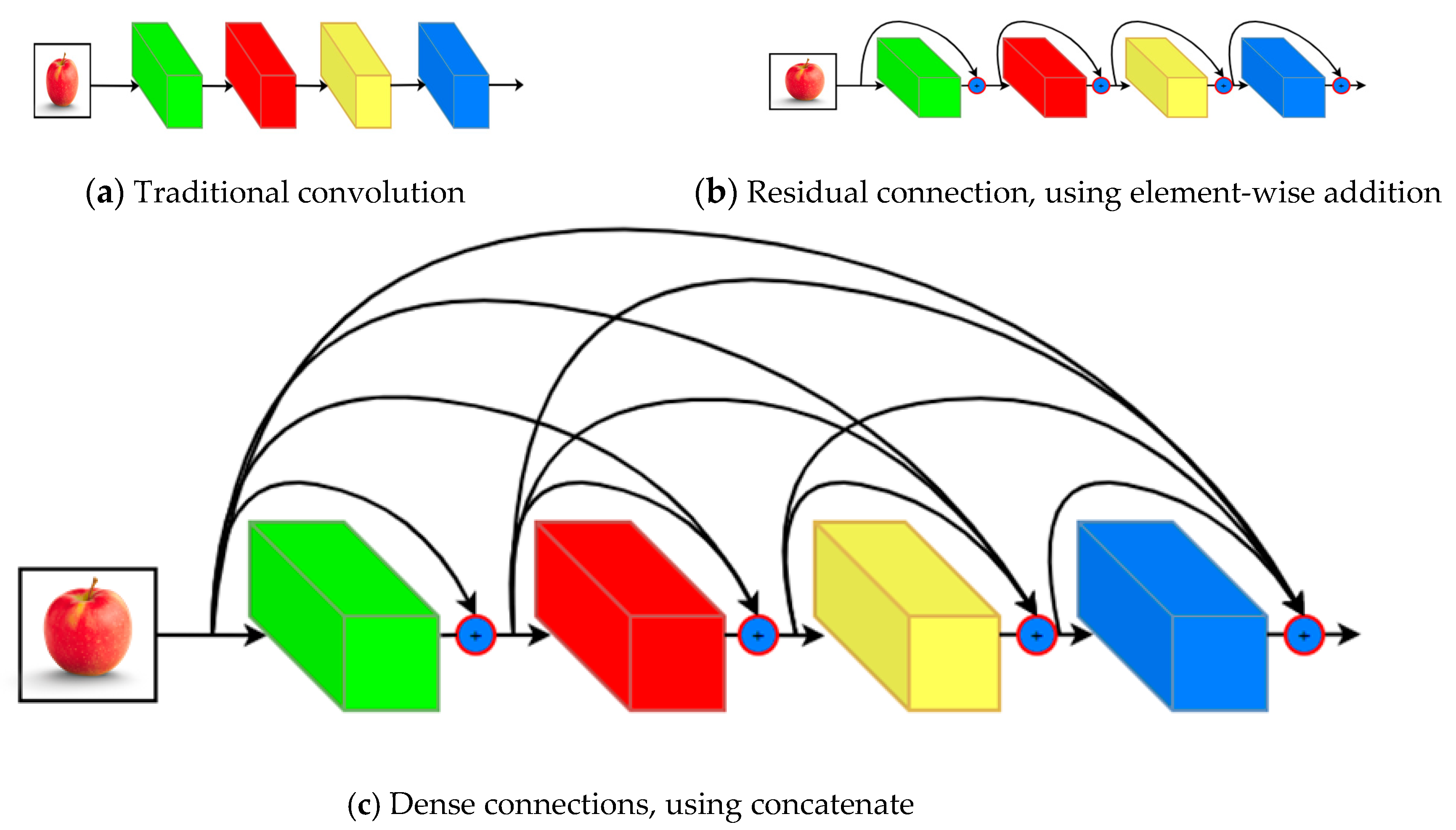
3.1. Skip Connection

Traditional feed-forward convolutional networks connect the output of the l^th layer as input to the ${\left(l + 1\right)}^{th}$ layer, which gives rise to the following layer transition: $x_l=H_l\left(x_{l-1}\right)$. The ResNet’s authors added a skip connection that bypasses the non-linear transformations with a function as identity as shown in Figure 1:

$$x_l=H_l\left(x_{l-1}\right)+x_{l-1}$$

(1)

Figure 1. Simple representation of types of convolutions from layer to layer, note that layers have the same height and width.

An advantage of ResNet was that the gradient can flow directly through the identity function from early, close to input layers to the subsequent layers.

3.2. Dense Connections

Huang et al. [11] introduced dense connections that connected every layer in feed-forward direction. Different from ResNet, DenseNet did not sum the output feature maps of the layer with the incoming feature maps but concatenated them instead. Consequently, the equation for the $l^{th}$ layer:

$$x_l=H_l\left(\left[x_0,x_1,\dots ,x_{l-1}\right]\right)$$

(2)

where $\left(\left[x_0,x_1,\dots ,x_{l-1}\right]\right)$ is the concatenation of output feature map of layers $0, 1,\dots , l-1$.

Since this grouping of feature maps cannot be done when the sizes of them are different, DenseNet is divided into Dense Blocks, where the dimensions of the feature maps remain constant within a block, but the number of filters changes between them. Huang et al. [11] also created Transition Layers, which stay between blocks and take care of the downsampling by applying a Batch Normalization (BN), a $1\times 1$ convolution and a $2\times 2$ pooling layers.

Another important feature of DenseNet is the growth rate. As defined in [11], the $l^{th}$ layer had $k_0+k\times \left(l-1\right)$ input feature map; where $k_0$ was the number of feature maps at input layer, and $k$ was the growth rate.

3.3. Depthwise Separable Convolution

Srivastava et al. [10] and Huang et al. [11] proposed Separable Convolutions layer (“s-conv” for short), which performed first a Depthwise Spatial Convolution (which acts on each input channel separately) followed by a pointwise convolution which mixes together the resulting output channels.

A standard 2D convolutional layer takes $D_H \times D_W \times M$ as input feature map I and produces a $D_h \times D_w \times N$ output feature map O where $D_W$ and $D_H$ are the spatial width and height of a input feature map, M is the number of input depth, $D_w$ and $D_h$ are the spatial width and height of a output feature map and N is the number of output depth.

Kernel K performs convolution on input feature map (with zero padding and stride one), has size $D_K \times D_K \times M\times N$, where $D_K$ is the spatial dimension of the kernel (assumed to be square) and M is the number of input channels and N is the number of output channels as defined. Normal convolutions have the computational cost of:

$$L_{conv2d}=D_K\times D_K\times M\times N\times D_h\times D_w$$

(3)

The computational cost depends multiplicatively on the number of input channels M, the number of output channels N, the kernel size $D_K \times D_K$ and the feature map size $D_h \times D_w$.

Depthwise Separable Convolution splits a kernel into 2 separate kernels that do two convolutions: the Depthwise Spatial Convolution and the pointwise convolution. Depthwise Spatial Convolution is the channel-wise $D_K \times D_K$ spatial convolution. Pointwise convolution is the $1\times 1$ convolution to change the dimension. Separable convolutions have the computational cost:

$$L_{separable conv2d}=D_K\times D_K\times M\times D_h\times D_w+M\times N\times D_h\times D_w$$

(4)

Performing division, the computational reduction is:

$$\frac{{\mathrm{L}}_{separable conv2d}}{{\mathrm{L}}_{conv2d}}=\frac{1}{N}+\frac{1}{{D_K}^2}$$

(5)

3.4. Formatting of Mathematical Components

DenseNet [11], U-Net [15] and V-Net [24] have showed that convolutional networks can be significantly deeper, more accurate, and simple to train if they contain shortcut connections between layers close to the input and ones close to the output.

Inspired by these ideas, we first create bottlenecked block with skip connection, dense connectivity and growth rate equaled to 32 similar to DenseNet’s architecture and connect every block to eaxh other in feed-forward fashion. We add longer skip connections to pass features from upper layers (blocks) to lower layers (blocks). Generally, the $t^{th}$ block receives the feature maps of all early blocks $n_0,n_1,\dots ,n_{t-1}$. The function of the $t^{th}$ layer is presented as follows:

$$n_t=H_{l,n_t}\left(x_{l,n_{t-1}}\right)+{{\displaystyle \sum }}_{i=0}^{t-1}{n}_i$$

(6)

where ${(t-1)}^{th}$ block has l layer.

We use 3 × 3 separable convolution layer instead of $3 \times 3$ normal convolution, as it reduces number of parameters as well as FLOPs, thus lowering computational effort.ơ

3.5. Bottlenecked Layers

It has been shown in [9,16] that a $1 \times 1$ convolution can be presented as bottleneck layer before each $3 \times 3$ convolution to reduce the number of input feature maps, therefore improving computational performance. We design our building blocks as this method, stacking $1 \times 1$ conv, $3 \times 3$ separable-conv, then $1 \times 1$ conv, where $1 \times 1$ conv(s) function to reducing and restore dimensions, while $3 \times 3$ s-conv(s) do the convolution with lower input/output dimensions.

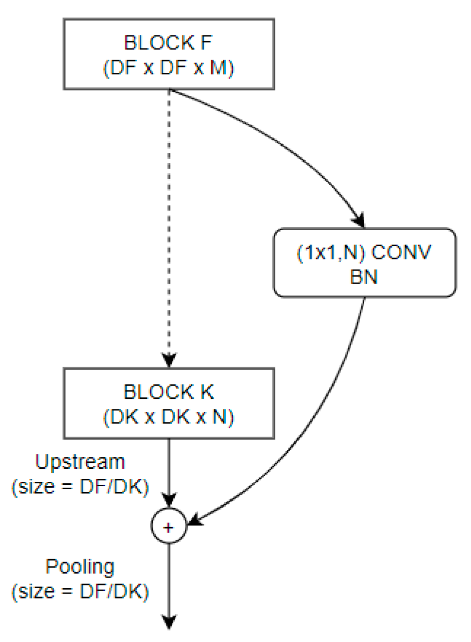
3.6. Upstream and Pooling Layers

An important aim of convolution networks is to downsample layers in which feature maps sizes change. To deal with the blocks’ depth difference, we add $1 \times 1$ conv to match block to block depth. Upstream2D and MaxPooling2D layers are added on the connections between blocks as shown in Figure 2.

Figure 2. Connection between 2 blocks with upstream and pooling layers (called Add block). BN denotes Batch Normalization and the normal line represents long skip connection between blocks while dash line states that there could be additional block(s) between block F and K.

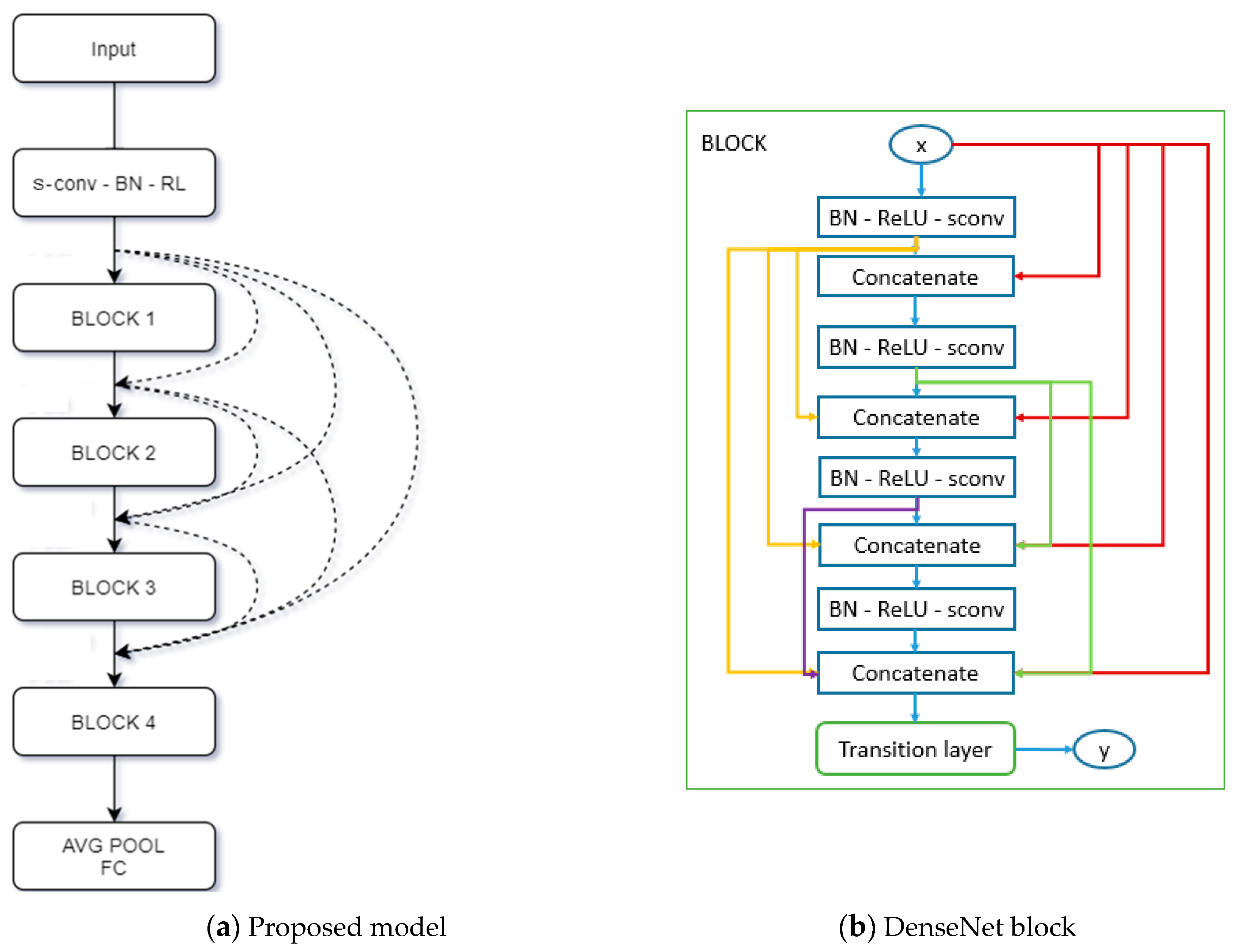
3.7. M-DenseNet Architecture

Figure 3 illustrates the simple M-DenseNet architecture. Similar to DenseNet, we create dense connection between layers in each block, then add transition layer(s) to perform downsampling. However, we change all $3 \times 3$ conv layers in DenseNet to s-conv layer, then add Add block as shown in Table 1.

Figure 3. An overview of model architecture. Note that the skip connections are created between blocks (layers with different shapes). Our model can be considered as a larger version of connection of DenseNet with separable convolution instead of normal 2D convolution.

Table 1. MDenseNet’s architectures.

Name	Size	M-DenseNet121	M-DenseNet169	M-DenseNet201
Separable-Conv2D	$112\times 112$	$7\times 7$ s-conv, stride = 2
MaxPool2D	$56\times 56$	$3\times 3$ max pool, stride = 2
Block 1	$56\times 56$	$\left[\begin{array}{c}1\times 1 conv\\ 3\times 3 s-conv\end{array}\right]\times 6$
Transition Layer 1	$56\times 56$	$1 \times 1$ conv
	$28\times 28$	$2 \times 2$ average pool, stride 2
Add block (0–1)	$56\times 56$	upsampling2d(size = 2), $1\times 1$ conv, maxpool2d
Block 2	$28\times 28$	$\left[\begin{array}{c}1\times 1 conv\\ 3\times 3 s-conv\end{array}\right]\times 12$
Transition Layer 2	$28\times 28$	$1 \times 1$ conv
	$14\times 14$	$2 \times 2$ average pool, stride 2
Add block (0-2)	$56\times 56$	upsampling2d(size = 4), $1\times 1$ conv, maxpool2d
Add block (1-2)	$28\times 28$	upsampling2d(size = 2), $1\times 1$ conv, maxpool2d
Block 3	$14\times 14$	$\left[\begin{array}{c}1\times 1 conv\\ 3\times 3 s-conv\end{array}\right]\times 24$	$\left[\begin{array}{c}1\times 1 conv\\ 3\times 3 s-conv\end{array}\right]\times 32$	$\left[\begin{array}{c}1\times 1 conv\\ 3\times 3 s-conv\end{array}\right]\times 48$
Transition Layer 3	$14\times 14$	$1 \times 1$conv
	$7\times 7$	$2 \times 2$ average pool, stride 2
Add block (0-3)	$56\times 56$	upsampling2d(size = 8), $1\times 1$ conv, maxpool2d
Add block (1-3)	$28\times 28$	upsampling2d(size = 4), $1\times 1$ conv, maxpool2d
Add block (2-3)	$14\times 14$	upsampling2d(size = 2), $1\times 1$ conv, maxpool2d
Block 4	$7\times 7$	$\left[\begin{array}{c}1\times 1 conv\\ 3\times 3 s-conv\end{array}\right]\times 16$	$\left[\begin{array}{c}1\times 1 conv\\ 3\times 3 s-conv\end{array}\right]\times 32$	$\left[\begin{array}{c}1\times 1 conv\\ 3\times 3 s-conv\end{array}\right]\times 32$
Global AvgPool2D
Dense (num_classes, SoftMax)

num_classes: number of classes.

Table 1 shows different configuration of the M-DenseNet. Blocks are shown in bracket with number of repetitions. Upsampling2d with $1\times 1$ conv2d helps add blocks match dimension. Introduced initially before the Block 1, a convolution with 64 output channels, $7\times 7$ kernel size and 2 strides are applied on the input image. The block architecture, as shown in Figure 2, follows the idea of Deeper Bottleneck Architectures [11]. Add block (m-n) means that we create long connection between block m and block n, block 0 is the output feature map of the first MaxPooling2D layer and block n is the output feature map of Transition Layer n^th.

4. Experiments and Results Analysis

4.1. Case Study on the Bamboo Strips Dataset

4.1.1. Build Dataset

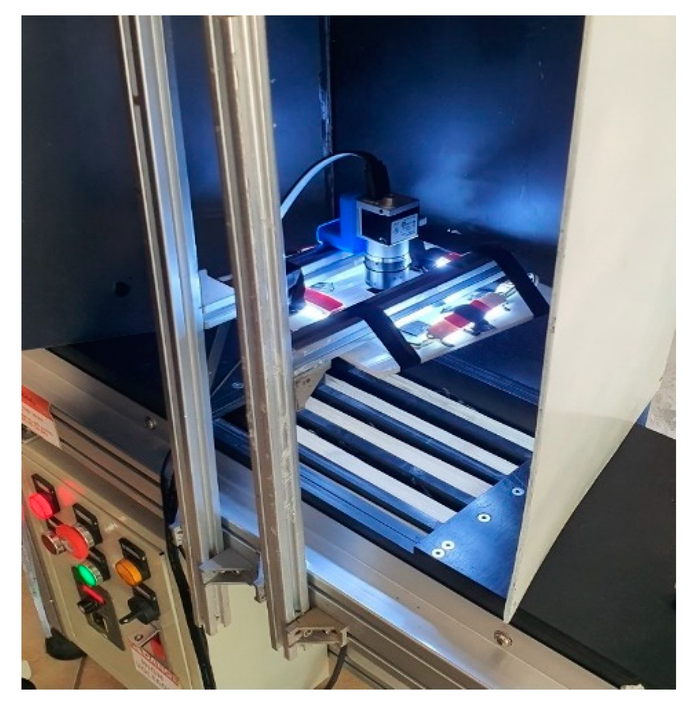
The Bamboo images are taken by using high speed Area Color camera (BASLER- acA1920--150uc, ~200 frames per second) with a lens of 8 mm focal length (TAMRON), a frame grabber and a PC. The camera is fixed above the bamboo strip and set focus on the surface. Because of the importance of keeping light in an undisturbed environment, a square shaped LED light is fixed above the bamboo strips. The type of lights, with the addition of a black box as shown in Figure 4 below, are effective against reflection and shadow, as well as the disturbing light from the environment.

Figure 4. Camera and light system.

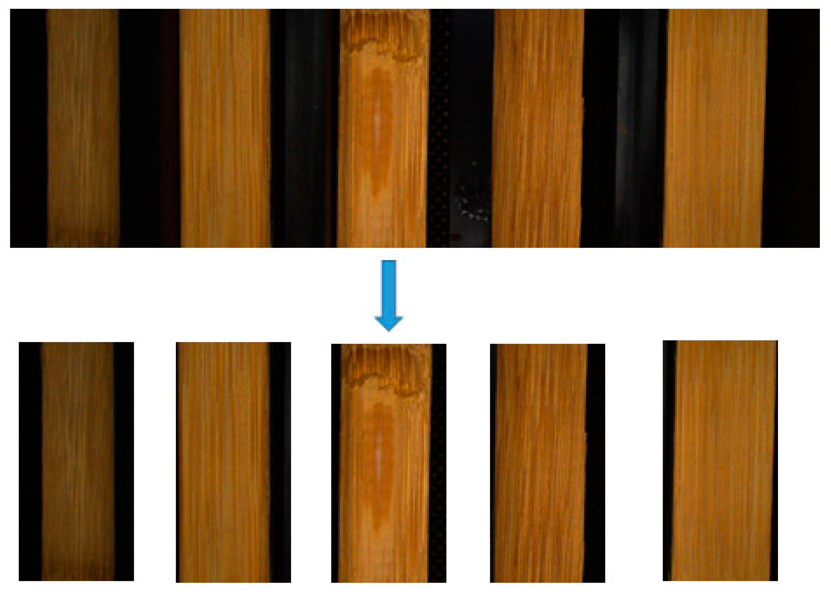
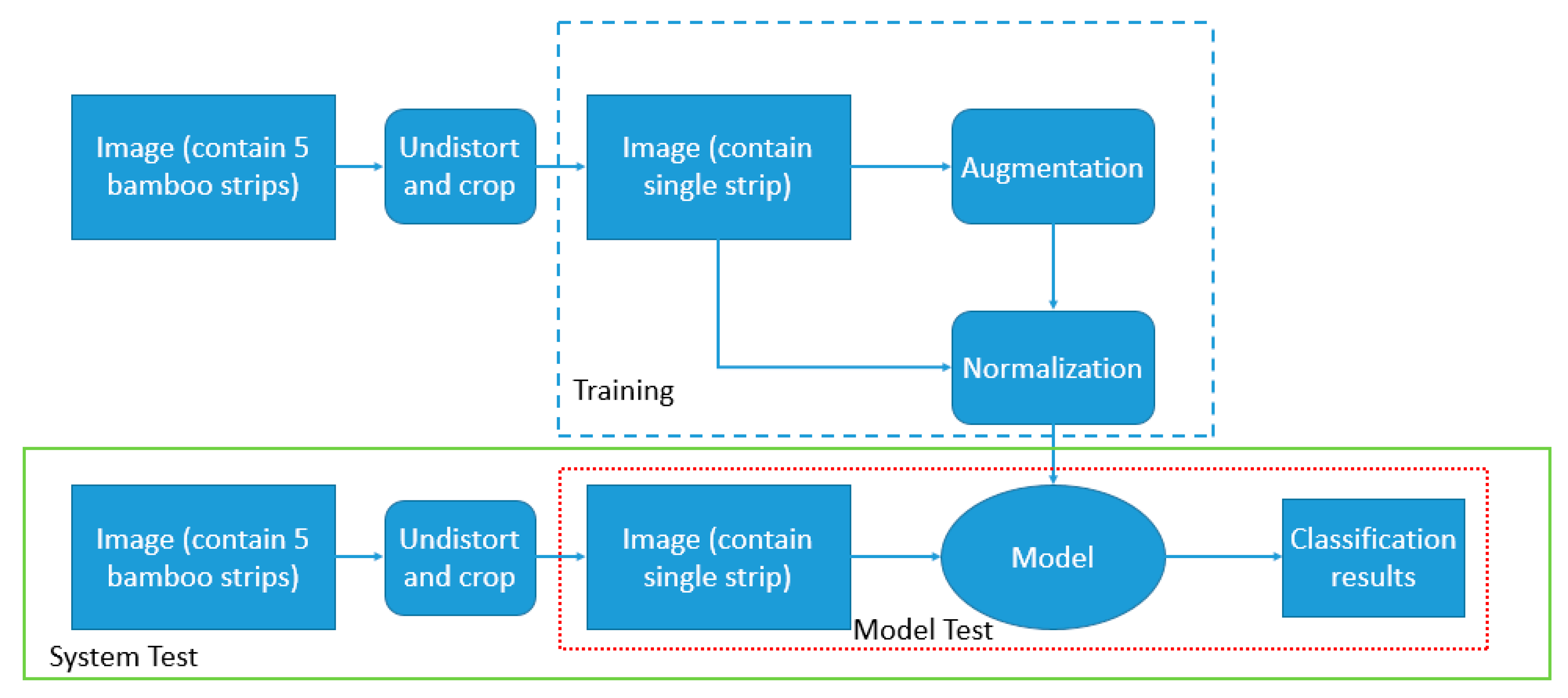
Typical bamboo strips have 2 cm width, so in order to improve production speed, we recorded images of five parallel strips over the conveyor. To deal with lens distortion, we calibrated the camera and obtain its matrix together with distortion coefficients, by the help of OpenCV library [25]. The images are then split into five equals parts (removing unwanted areas), containing each bamboo strip with similar height and width, as described in Figure 5.

Figure 5. Initial image to 5 divided images (from top to bottom).

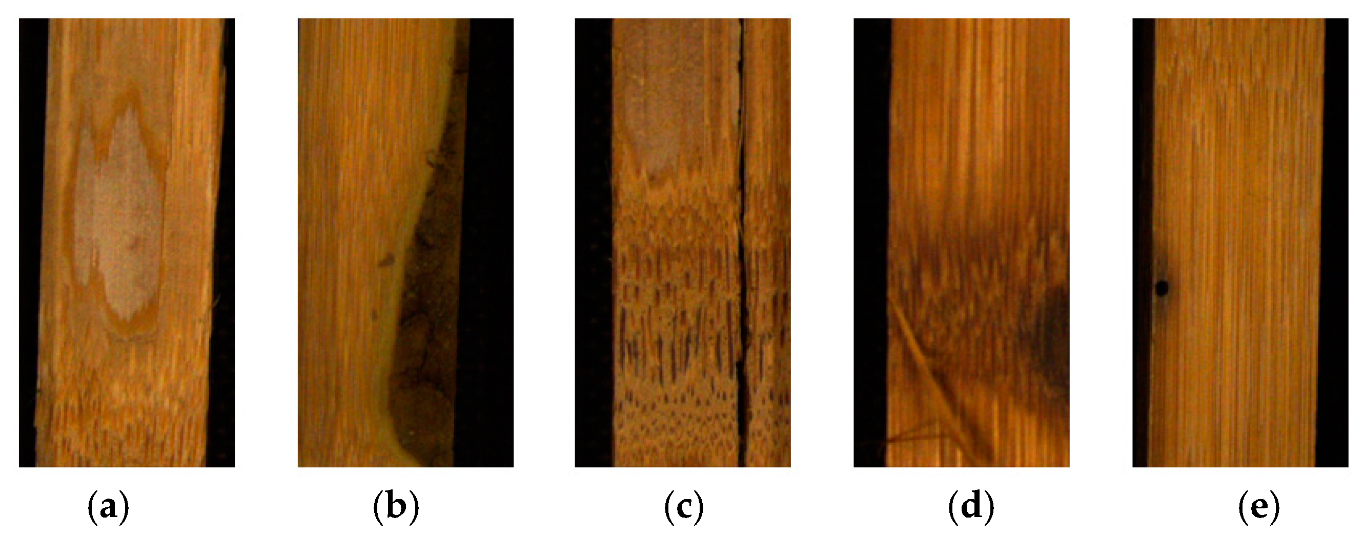
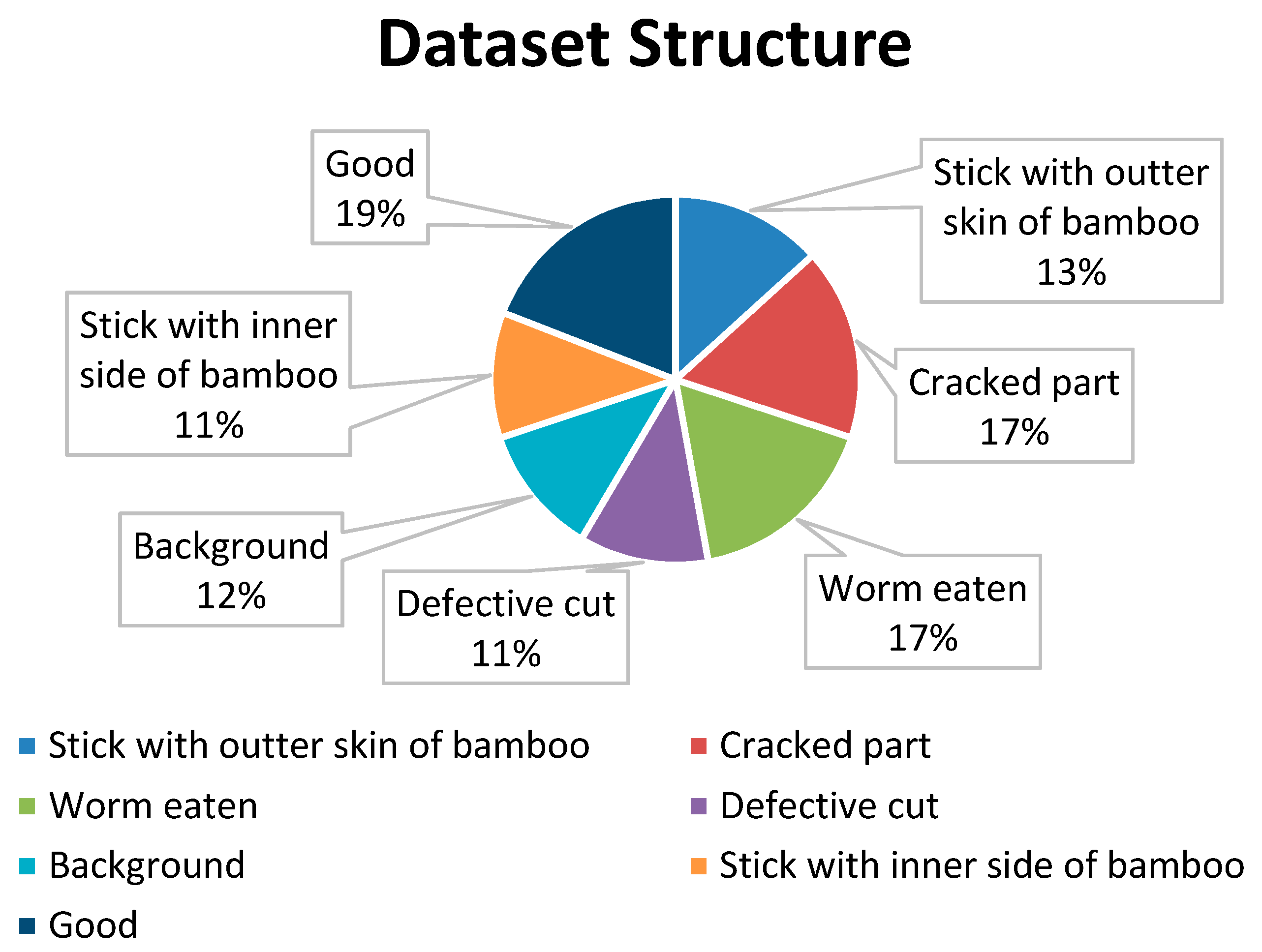
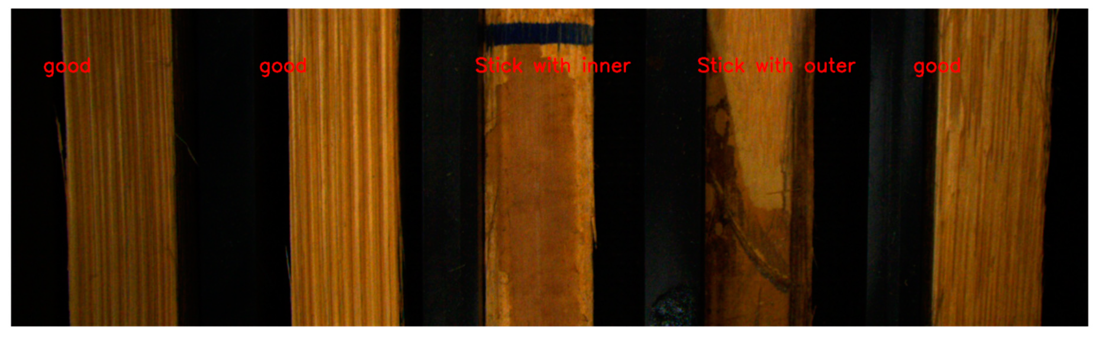
We build a Bamboo strips dataset (about 25,000 images), which contains seven classes that are classified manually. The dataset can be accessed at https://github.com/hieuth133/Bamboo, accessed on 24 January 2021. The images shape is $260\times 500\times 3$ and the dataset contains seven classes: one for good bamboo strips, five classes contain non-qualified bamboo strips images (detailed in Section 3.1), and the last one is background (images of conveyor). Example of bamboo defect images are shown in Figure 6. Images are cropped to $224\times 224\times 3$ with per-pixel mean subtracted. Because the number of images containing defect is minimal compared to the good bamboo strips images, we upsample the defect bamboo classes by using image augmentation. Using Keras ImageDataGenerator library [26], we generate new images by horizontal and vertical flipping, rotating (±2 degree), shifting height and width, changing brightness. Both original and generated images are used together to form the Bamboo dataset. Figure 7 points out the distribution of number of images from seven classes in percentages.

Figure 6. Example of non-qualified bamboo strips class images, from left to right: (a) stick with inner side, (b) stick with outer skin, (c) cracked, (d) defective cut, (e) worm eaten.

Figure 7. Bamboo dataset structure.

4.1.2. Training Model

We evaluate the M-DenseNet on our Bamboo strips dataset, as shown in Figure 8.

Figure 8. Training and testing method for Bamboo image classification.

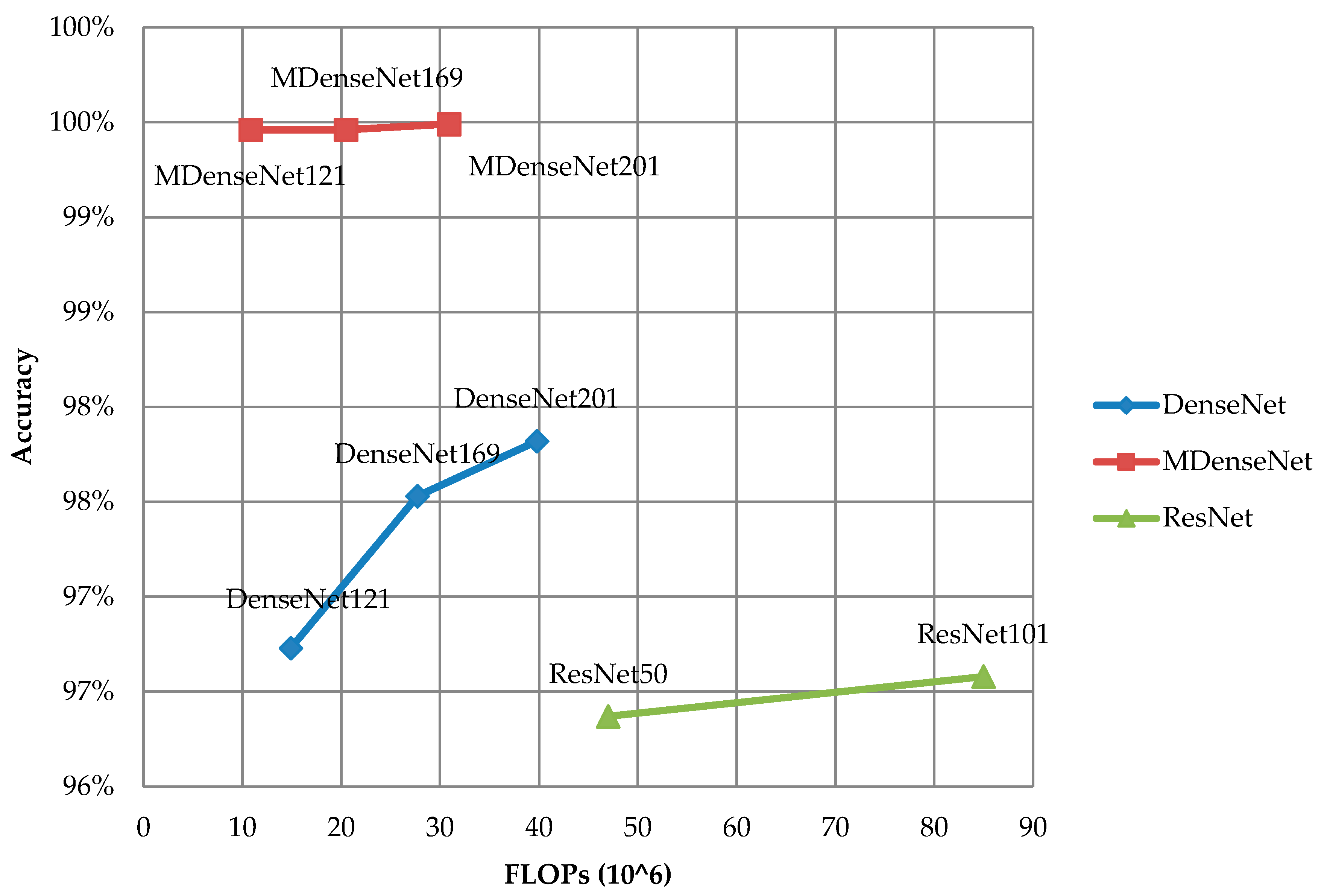
We choose batch size of 32 for 30 epochs and stochastic gradient descent (SGD), with learning rate equal to ${10}^{-3}$, divided by 10 at epoch 10 and 20, weight decay = ${10}^{-6}$, momentum = 0.9, and Nesterov momentum is applied. Training time is about 3 hours on Tesla V100-SXM2 with 16GB of VRAM, and computation capability is 7.0. Table 2 shows the results of M-DenseNet(s), DenseNet(s) and ResNet(s) trained on Bamboo dataset. All models’ accuracies are qualified for bamboo industry (≥95%), and M-DenseNet utilizes parameters more efficient than other models, which appears in Figure 9 and image prediction as shown in Figure 10. Model accuracy is defined as an average number of items correctly identified as either truly positive or truly negative out of the total number of items:

$$\frac{{\sum }_{i=1}^k\frac{t{p}_i+t{n}_i}{t{p}_i+t{n}_i+f{p}_i+f{n}_i}}{k}$$

(7)

where k is number of classes, “t” is true, “f” is false, “p” is positive and “n” is negative.

Table 2. Accuracy and floating-point operations per second (FLOPs) achieve by M-DenseNet in comparison with the other models.

Model	Parameter $\left({10}^6\right)$	FLOPs $\left({10}^6\right)$	Accuracy on Validation Set (%)
DenseNet121	7.05	14.97	96.73
DenseNet169	12.66	27.76	98.16
DenseNet201	18.34	39.90	97.83
ResNet50	23.50	47.00	96.37
ResNet101	42.00	85.00	96.58
MDenseNet121	5.51	10.83	99.46
MDenseNett169	10.42	20.50	99.46
MDenseNet201	15.71	30.94	99.49

Numbers in bold represent best result.

Figure 9. Comparison of accuracy and FLOPs between M-DenseNet, DenseNet and ResNet.

Figure 10. Image prediction final result.

4.2. Case Study on the Reduced Version of ImageNet

We also test the M-DenseNet and DenseNet families without/with long skip connection and s-conv. We use another dataset, which is a reduced version of ImageNet [27] with 100 classes and about 500 images in each class. The dataset is also accessible via the same github link above (Section 4.1.1). All models are trained by the same technique with extra augmentation [28,29,30] and normalization [31]; batch size is 32, Adam optimizer, 60 epochs and learning rate is ${10}^{-3}$.

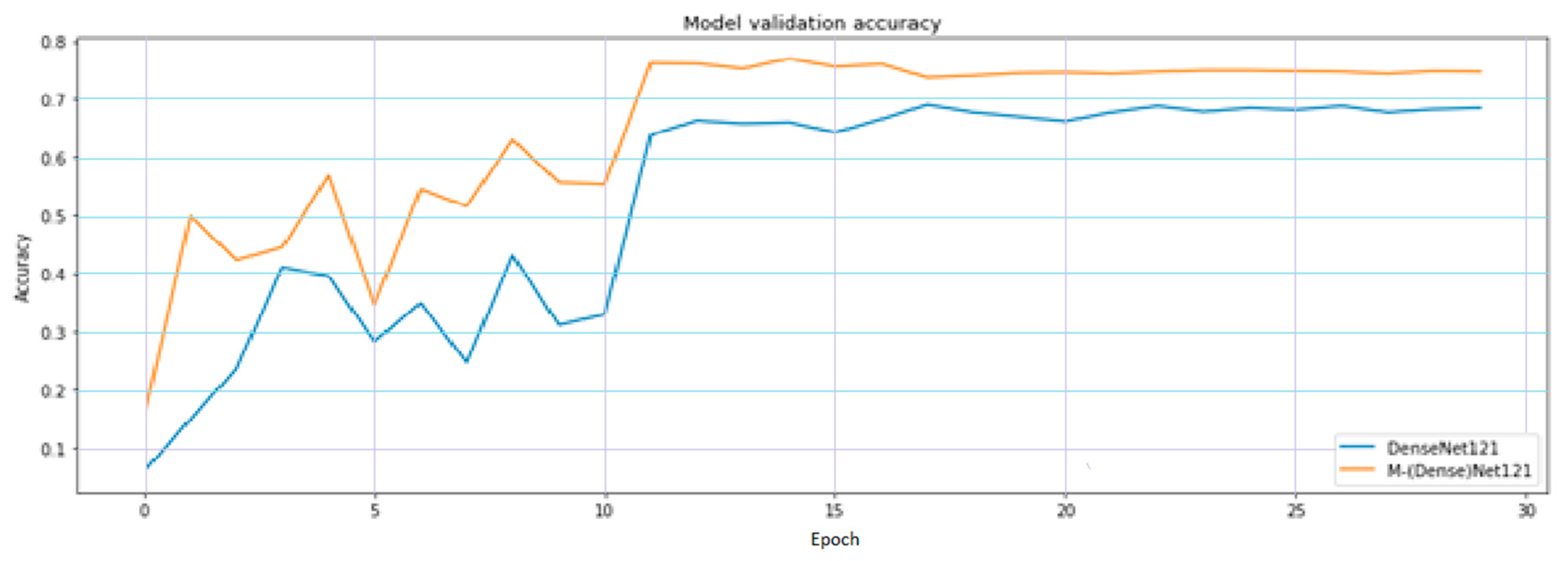
Table 3 presents the value of accuracy and FLOPs in comparison between DenseNet and M-DenseNet. By observation, models with long skip connection converge faster, as shown in Figure 11 and has a better overall result. Parameters and FLOPs of M-DenseNet family equal roughly 80% of original DenseNet, while the accuracy increases about 3–5%.

Table 3. Accuracy and FLOPs achieved by M-DenseNet in comparison with DenseNet.

Model	Parameter $\left({10}^6\right)$	FLOPS $\left({10}^6\right)$	Accuracy on Validation set (%)
DenseNet121	7.14	14.11	73.72
DenseNet169	12.80	25.30	74.54
DenseNet201	18.51	36.57	75.65
M-DenseNet121	5.50	10.83	78.56
M-DenseNet169	10.41	20.50	78.86
M-DenseNet201	15.71	30.94	79.42

Numbers in bold represent best result.

Figure 11. Comparison between DenseNet121 and M-DenseNet121 in terms of model validation accuracy from epoch 0 to 30.

Testing usage with other models: We make modifications to other models, similar to what we have done to create MDenseNet in Section 3.7. The models are EfficientNet [23] and MobileNet v1, v2, v3 [13,18,19]. We use a reduced version of ImageNet and training technique the same as that explained in Section 4.2. Below is the detail of comparison.

Figure 12 and Figure 13 point out that our modifying models perform better than the original ones with small decrease in FLOPs (6-3% for MobileNet and 2-1% for EfficientNet). This proves the effectiveness of the long skip connections to performance of CNN.

Figure 12. Comparison between MobileNet and (M) MobileNet (V1–V3, right to left, respectively).

Figure 13. Comparison between EfficientNet and (M) EfficientNet (B0–B4, left to right, respectively).

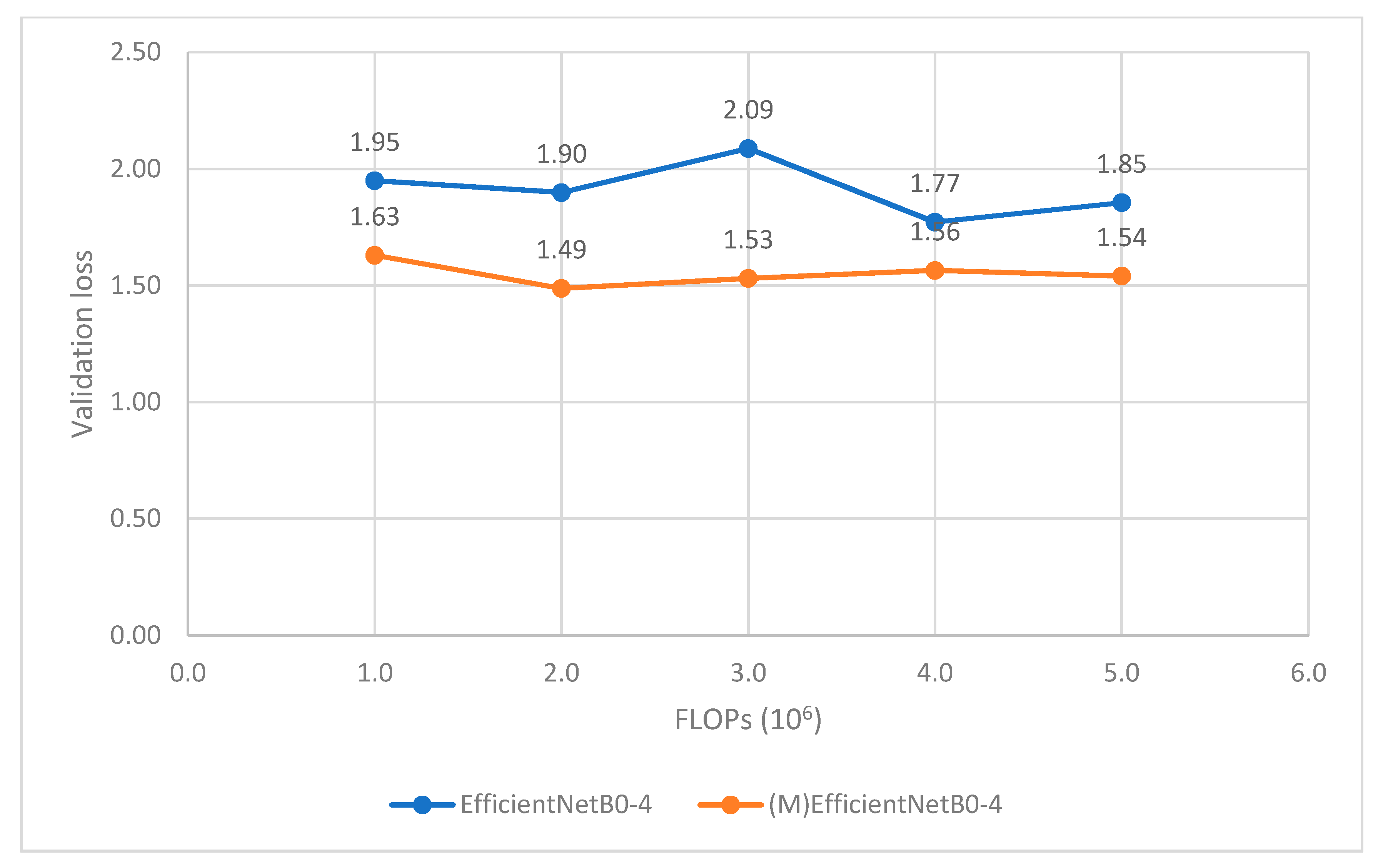
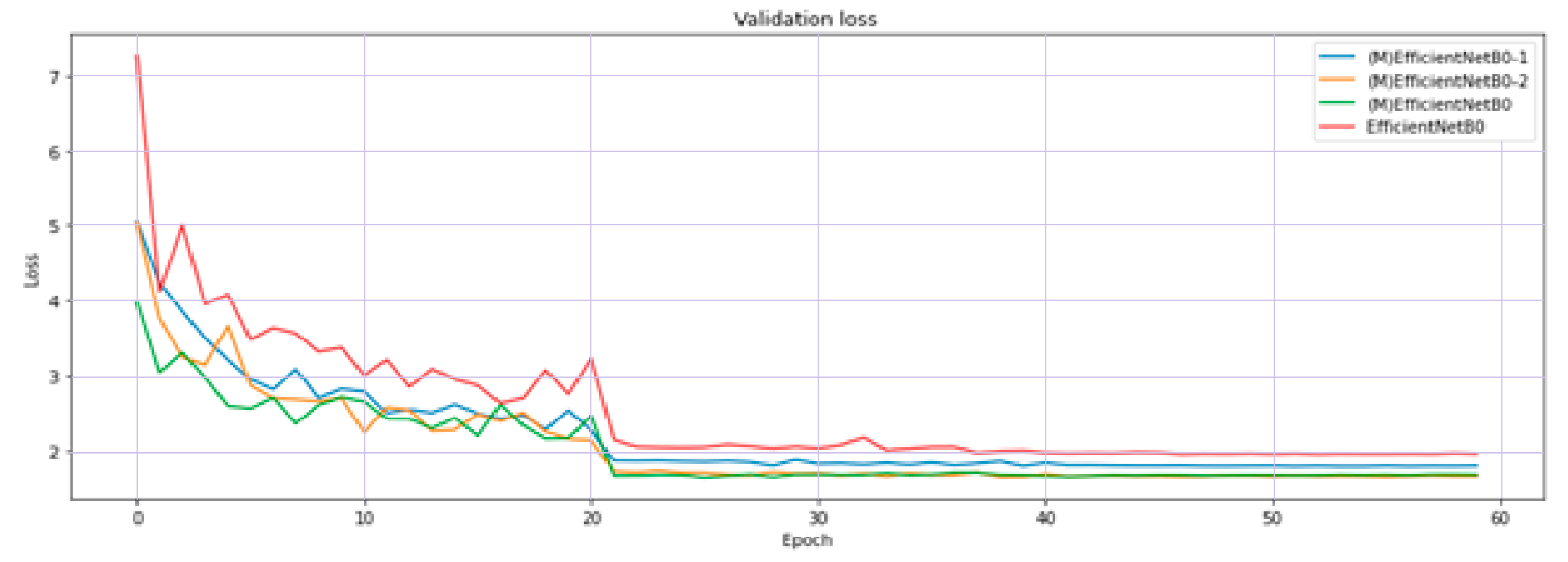
4.3. Ablation Study

We conducted an ablation study to point out the effectiveness of long skip connection to the performance of the models. We used EfficientNet B0 and three modified models based on EfficientNet B0 for testing.

The configuration for training and dataset is the same as that explained in Section 4.2. Figure 14 shows the validation loss while training 4 models in 60 epochs. Models with more long skip connections perform better than ones with less long connections.

Figure 14. Validation loss comparison between EfficientNet B0 and our modification based on EfficientNet B0 (3 models); EfficientNet B0 is the base model; (M) EfficientNet B0 is our modification model, add blocks are added that connect all blocks similar to DenseNet (Figure 3.b); (M) EfficientNet B0-1 has only connections between consecutive blocks (Block N - Block N+1); (M) EfficientNet B0-2 has connections between consecutive blocks and blocks separated by 1 block (Block N – Block N+1; Block N – Block N+2).

5. Discussion

As noted above, the modification adds to the model and turns it into a larger version of DenseNet. The upgrade seems to be small but it led to notable consequences. We present a few discussions and experiments to prove the efficiency of our proposed method.

Feature reuse: Generally, the feature maps close to the input detect small or fine-grained detail, whereas feature maps close to the output of the model capture more general features. The connection between blocks encourages layers to learn both small detail and general nature of the object. The ablation study also proves the effect of skip connections that is more connections results in better performance.

Adaptability: The method of adding long skip connections has the ability to fit well to other models, from lightweight one like MobileNet family to well-designed EfficientNet family. Comparative experiments show that the modified models converge faster and have better performance.

Difficulty: In order to perform long skip connection between layers having different size, we have to equal the shape of two layers (detail in Section 3.6). This task can consume large GPU memory capacity and is unable to work with small size GPU, as the shape of feature map of the long skip connection layer is very large.

6. Conclusions

In this paper, we have proposed a modification to improve the performance of CNNs by using the effect of long skip connections. It creates long connections between blocks of layers with different sizes of feature map. In our experiment, the models with long skip connections tend to converge faster, without overfitting. The MDenseNet 121 model achieves higher validation accuracy while it has about 75% of weights and FLOPs in comparison to the original DenseNet 121. Adding long skip connections also helps MobileNets and EfficientNets families to improve their performances (tested with a reduced version of ImageNet).

The models with long skip connections have benefits in comparison to their counterparts, as it enhances feature reuse throughout the models, encourage models to learn both the fine details (coming from layers close to input) and the more general details (coming from layers close to output) of the objects. Moreover, the proposed modification is highly adaptable to many models, from lightweight to heavily parameterized models. As ad limitation, we experience difficulty in training big models, which is a result of the large shape of the feature map in the skip connection.

We will try to control the amount of knowledge when performing long skip connection in further experiments. In future work, we will explore this architecture with deeper layers, while maintaining its performance to apply to different tasks such as segmentation or object detection.