Artificial Intelligence for Creating Low Latency and Predictive Intrusion Detection with Security Enhancement in Power Systems

Abstract

Advancement in network technology has vastly increased the usage of the Internet. Consequently, there has been a rise in traffic volume and data sharing. This has made securing a network from sophisticated intrusion attacks very important to preserve users’ information and privacy. Our research focuses on combating and detecting intrusion attacks and preserving the integrity of online systems. In our research we first create a benchmark model for detecting intrusions and then employ various combinations of feature selection techniques based upon ensemble machine learning algorithms to improve the performance of the intrusion detection system. The performance of our model was investigated using three evaluation metrics namely: elimination time, accuracy and F1-score. The results of the experiment indicated that the random forest feature selection technique had the minimum elimination time, whereas the support vector machine model had the best accuracy and F1-score. Therefore, conclusive evidence could be drawn that the combination of random forest and support vector machine is suitable for low latency and highly accurate intrusion detection systems.

1. Introduction

An exponential increase has been noticed in the number of Internet users since the last decade. Latest data reveal that there were 5.098 billion Internet users in December 2020, which equals to 64.7% of the population on the earth [1]. Consequently, the Internet is the most popular medium to connect globally and the largest knowledge repository available. It facilitates communication via different techniques such as text, video or audio, therefore making a lot of private user information available on various platforms. The introduction of IoT technology with a combination of advanced network technology has become an integrated part of humankind. The devices include smart home appliances, smart grids. These also act as building blocks of the vision for smart cities. Usage of these devices support continuous data transfer without any human intervention [2].

This has created an exponential rise in the IoT industry. A report on IoT analytics indicates that the number of IoT devices is expected to surpass 35 billion by 2025, whereas 22 billion devices were already connected in 2018 [3]. This increase corresponds to the fact that the IoT is extensively leveraged to solve problems in various domains such as smart cities, garbage management system, smart traffic management system, water supply and monitoring air standards to control pollution [4]. An IoT-based development can be seen in smart home automation appliances, smart cars, industrial M-to-M communication and robotic surveillance in the military [4,5]. Pertaining to these applications of the IoT in various domains, there is a huge amount of data transfer. This makes the devices susceptible to intrusions, as cyber criminals often try to gain control in illicit ways.

The end goal of intrusions is to access a user’s confidential information. Cyber criminals manipulate confidential information to gain remote access to the devices [6]. This may pave the way for intruders to perform illegal activities using a fake identity and possibly financial loss [7].

Some of the frequent techniques employed by intruders are discussed below:

• Malware—malware is just code packed with malicious content. About 92% of malware is deployed via email attachments and the rest as downloadable content. The primary motivation of using malware is to infect the device and steal or destroy information. In November 2020 alone, about 113 million new malware programs were reported [8].
• Phishing—it simply is an act of posing as a legitimate organization or person and asking users for sensitive information. According to the APWG report in the Q4 of 2020, 22.5% of the phishing activities targeted financial institutions, 22% of them involved SAAS/webmail and 15.2% of them were involved in payment activities [9].
• Password attack—these include frequent dictionary attacks or keyloggers to gain access to users’ passwords. Password decryption is employed to gain the original password from the hashed password. Therefore, it is essential to have a password combination consisting of alphabets, numeric and special characters.
• DDoS—a distributed denial-of-service interrupts the proper functioning of Internet-connected devices. It continuously sends fake requests to the server, consequently increasing the load on the server. Hence, when a legitimate user sends a request to the server, the server is not able to respond to valid requests. If the same activity is performed by a large number of infected devices, from which millions of requests are sent to the server and if a valid user tries to request on the server, the server is unable to respond due to high traffic or malicious requests. In a report by Netscout, 929,000 DDoS attacks were recorded within 31 days, in April-May 2020 [10].

The statistics suggest an increasing number of intrusion attacks. These attacks are successful due to a lack of awareness and proper knowledge [11]. To mitigate this important problem, a robust intrusion detection system needs to be installed in network-connected devices that continuously monitor the network traffic and data packets coming from the server, which acts as a gateway, where the gateway is responsible for analysing the data packet for potential threats [12,13].

The high-level architecture of an intrusion detection system is shown in Figure 1. It shows how the request from the user is passed to the intrusion detection system, which analyses it and classifies it as safe traffic or attempts to intrude into the network. Various classification algorithms are used to classify the incoming packets into normal and anomaly classes. An IDS monitors all packets, analyses them and if they look like previous attacking patterns, classify them as normal and anomaly, according to their behaviour.

2. Related and Background Work

In this section, we discuss the existing research in the domain of intrusion detection. We briefly also discussed the formal methodology, algorithms and results achieved by various researchers from research previously conducted.

In this paper, M. Alkasassbeh et al. [14] proposed a model for intrusion detection. The KDD dataset was used for experiments with 60,000 randomized instances. J48, MLP and Bayes network algorithms were employed to model the classification problem. The J48 algorithm reported the best results with an accuracy of 93.1083% and true positive rate of 0.93.

An in-depth comparative analysis between Bayes net, logistic regression, IBK, J48, PART, JRip, random tree, RePTree and random forest combined with a 10-fold cross-validation was also performed by S. Choudhury et al. [15]. They reported a highest accuracy score of 91.523%.

M. Belouch et al. [16] in their paper leveraged Apache Spark to employ four classifiers support vector machine, naive Bayes, decision tree and random forest. They experimented using the UNSW-NB15 dataset with all 42 features to detect intrusion. Evaluation metrics such as accuracy, sensitivity, specificity, training time and prediction time were used for comparing algorithms. Results indicated that random forest performed the best by achieving the highest accuracy score of 97.49%.

In another research, a hidden naive Bayes classifier was used by L. Koc et al. [17] for intrusion detection. It was compared with other classification algorithms. Moreover, the hidden naive Bayes classifier was found to perform better than the naive Bayes algorithm as it achieved an accuracy score of 93.72%.

In their paper, T. A. Tang et al. [18] proposed a deep neural network (DNN) model for intrusion detection. They used the NSL-KDD dataset for training the models. They selected only 6 out of 41 features. In this approach, they achieved an accuracy of 75.75%. Further, they compared the performance of this approach with another classification algorithm and found a random tree as the best performing algorithm with an accuracy 81.59%.

D. Prabakar et al. [19] proposed an enhanced feature selection technique named simulating annealing, then they used an SVM classifier for intrusion detection. They used the NDL-KDD’99 dataset to train the model. The results of the proposed method were compared with previously presented results using GWO-SVM and PSO-SVM classifiers and gained 8.71% better accuracy and 43.64% lesser execution time.

In their paper, S. Rajagopal et al. [20] proposed a model to detect network intrusions. Two famous heterogeneous datasets, UNSW NB-15 and UGR’16, were used for the model. A stack-based meta classification technique was used for classification. The results of the model show this approach as a good ensemble classification technique; they achieved an accuracy of 94% and 97.19% for the UNSW NB-15 and UGR’16 datasets, respectively.

In [21], T. Ambwani proposed a multiclass classification approach using support vector machine classifiers for intrusion detection and misuse detection. They used the KDD’19 dataset for their experiment. The work achieved 91.6738% of accuracy while performing a 23-class classification and the lowest cost for each test sample was 0.252854. They found SVM was the better performing algorithm for intrusion detection tasks in comparison with artificial neural networks.

Pertaining to the studies that have been conducted in the past, in our research we aim to identify the following:

• Experiment with various ensemble feature selection techniques to identify the best set of features.
• Build a baseline model to set a benchmark for future studies.
• Analyse the performance of feature selection techniques based upon the time taken to select a particular set of features. This is particularly essential for building a low latency real-time system.

In this paper, the authors present the major contributions of the work to build an accurate and fast intrusion detection system. Secondly, it is important for an intrusion detection system to identify highly important features from the data for the prediction. This helps in making a low latency system for real-time deployment, which is very essential considering the work. Thirdly, the amount of data being generated is increasing at a steady rate as the number of Internet users rises.

The rest of the paper is structured as follows: Section 2 describes the material and methods adopted for the experimentation along with the dataset and approach used in this work. Section 4 analyses the results of the approach undertaken to build the model and finally Section 5 concludes the paper.

3. Materials and Methods

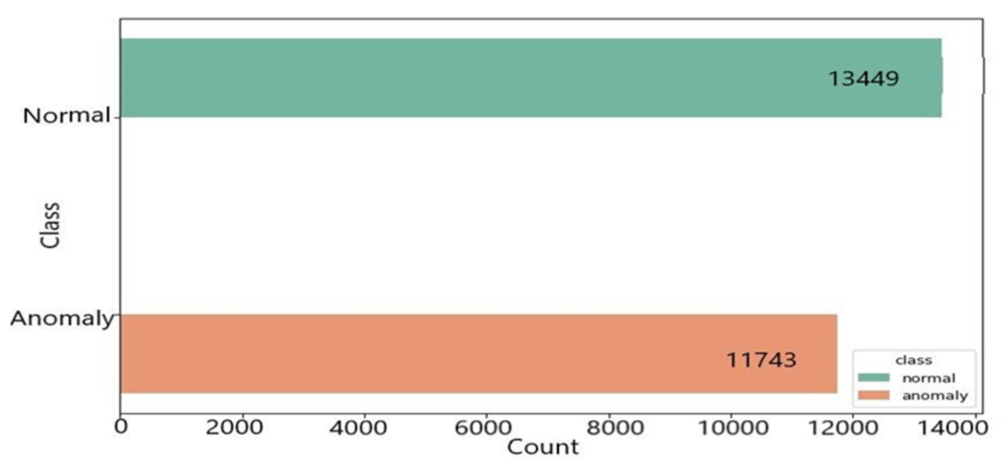
Intrusion detection systems analyse the requests from different users, which are passed to the classifier, whose purpose is to determine whether it is safe traffic or attempts to intrude the network. There have been a variety of algorithms used for such intention to classify the incoming packets in normal and anomaly classes. An IDS monitors all packets, analyses them and if they look like previous attacking patterns, classify them as normal or anomalous, according to their behaviour.

3.1. Used Dataset

The network intrusion detection dataset from Kaggle was used for training and testing the model [22]. The dataset consisted of intrusion data simulated in a military environment, where a US airline LAN was blasted with multiple intrusion attacks. The independent features of the dataset initially consisted of 38 numerical and 3 categorical features. The dependent feature consisted of two classes, namely: normal and anomaly. The anomaly class indicates an intrusion attack while the normal class means a safe network. The total number of occurrences of both classes are shown in Figure 2. The difference between the number of instances of the two classes is 1706, which is just 6.77% of the total number of instances, which is comparatively very small, and hence the dataset can be considered as balanced.

3.2. Algorithms

3.2.1. Random Forest (RF)

The random forest algorithm is an ensemble bagging technique, in which final prediction is made by selecting the majority of results from multiple decision trees. Random forests are used for classification and regression problems. The random forest algorithm gives a result based on the majority of decisions given by multiple decision trees. The forest term refers to the multiple trees whereas random refers to the random selection of input features on each decision tree. This algorithm uses raw sampling with replacement as an input. Inputs to each decision tree may be repeated, but repetition may lead to a decrement in the accuracy of the algorithm. While predicting results on a decision tree, if a small part of the dataset is replaced, then a high variance problem occurs which may change the actual prediction. In random forests, the prediction based on multiple parameters from the dataset may not have a major impact on the overall prediction of the model. The accuracy of random forest algorithms is much better than that of decision trees.

In order to give predictions on decision trees, the GINI IMPURITY and ENTROPY are calculated for optimal classification into classes on a node.

$$GINIIMPURITY=1-{{\displaystyle \sum }}_{i=1}^N{\left(P_i\right)}^2$$

(1)

where N represents the number of classes and P_i represents the probability of a class over a given input.

The GINI IMPURITY calculates the probability of misclassification of a class on a node.

$$ENTROPY=-{{\displaystyle \sum }}_{i=1}^{N}Pi\ast log2\left(Pi\right)$$

(2)

where N represents the number of classes in which the input data are being classified and $Pi$ represents the probability of a class over a given input. The ENTROPY is calculated for optimal classification into classes on each node. Each decision tree predicts an output based on given random inputs from a dataset. Random forests predict the result based on the majority of decisions taken by their decision trees on the same dataset.

3.2.2. Logistic Regression (LR)

It is a supervised learning method and is generally used for binary classification of dependent categorical features [23,24]. Algorithms predict their output based on dependent variables. Logistic regression uses a logistic curve, i.e., an “S”-shaped curve, for the separation of data points. Logistic regression predicts the probability of classification by drawing a decision boundary made by drawing a logistic curve. The logistic function is also known as a sigmoid function.

$$S\left(x\right)=\frac{1}{1+e-x}$$

(3)

The sigmoid function requires a real number as an input and gives an output in the range 0 to 1. The output of the sigmoid function is a probability for the classification. If $S\left(x\right)$ < 0.5, then the input data are classified in class A and if $S\left(x\right)$ > 0.5, then class B is assigned.

3.2.3. Support Vector Machine (SVM)

It is a supervised machine learning technique used in both classification and regression problems [25]. Generally, an SVM is used for classification problems. An SVM classifies the data into the given classes by drawing a separating line or separating planes between data points of each class. The best separating line is known as a hyperplane and the nearest data points from the hyperplane of each class are known as support vectors. Planes parallel to the hyperplane and passing through these support vectors are known as marginal planes. For the best possible classification, an SVM’s goals are to maximize the distance between both marginal planes.

The equation of the hyperplane is:

$$W^T\left(y\right)+c=0$$

(4)

where $c$ is a constant.

To calculate the distance of the data point from the hyperplane, let $\Phi \left(y\right)$ be a data point vector from the hyperplane.

$$d_H\left(\Phi \left(y_0\right)\right)=\frac{\left|W^T\Phi \left(y_0\right)+c \right| }{\Vert w\Vert }$$

(5)

where $\Vert w\Vert$ is the Euclidean norm of $w$.

Since support vectors are the nearest point from the hyperplane, we can calculate the distance for the support vector by minimizing Equation (5).

$$d_H{\left(\Phi \left(y_0\right)\right)}_{min}=min\left(\frac{\left|W^T\Phi \left(y_0\right)+c \right| }{\Vert w\Vert }\right)$$

(6)

The goal of an SVM is to maximize the minimum distance of the data points from the hyperplane.

$$w^{\ast }=\left(min\left(\frac{\left|W^T\Phi \left(y_0\right)+c \right| }{\Vert w\Vert }\right)\right)$$

(7)

$$w^{\ast }=d_H{\left(\Phi \left(y_0\right)\right)}_{min}$$

(8)

As $w^{\ast }$ in Equation (7) increases, optimal classification occurs among the given class labels.

3.3. Analysis Model

This subsection discusses the process workflow of our analysis and model building. This subsection was performed into a two-phase data analysis, which is explained in detail below.

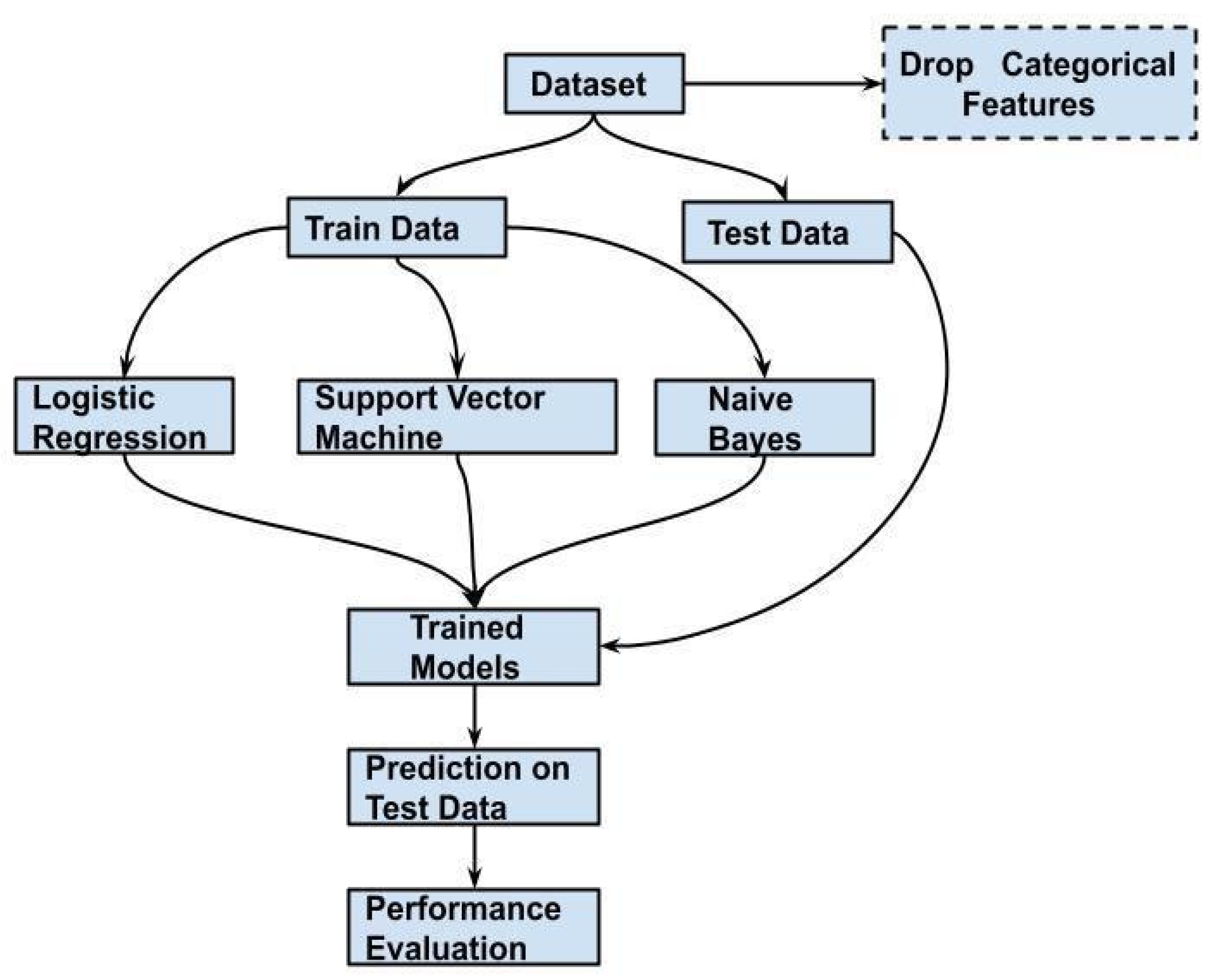
3.3.1. Baseline Model

Initially a baseline model was simulated for comparison purpose; this was particularly necessary to establish a benchmark for comparing the results of our proposed model and reporting improvements across various evaluation metrics. The workflow of the baseline model is shown in Figure 3.

Figure 3 shows the baseline model for the loading and division of the dataset into a 70-30 train-test data split. It does not consider the three categorical features from our data, namely: protocol type, service and flag from our feature set. The categorical features were removed as we performed no feature preprocessing for our baseline model, and hence only the remaining 38 quantitative features could be used as inputs.

Then, we used logistic regression (LR), support vector machine (SVM) and naive Bayes (NB) to train our model and finally tested the performance of our model using the test data as depicted in Figure 3 and Figure 4. The quantitative results of the baseline model obtained by calculating evaluation metrics are discussed in the result and analysis section of the paper.

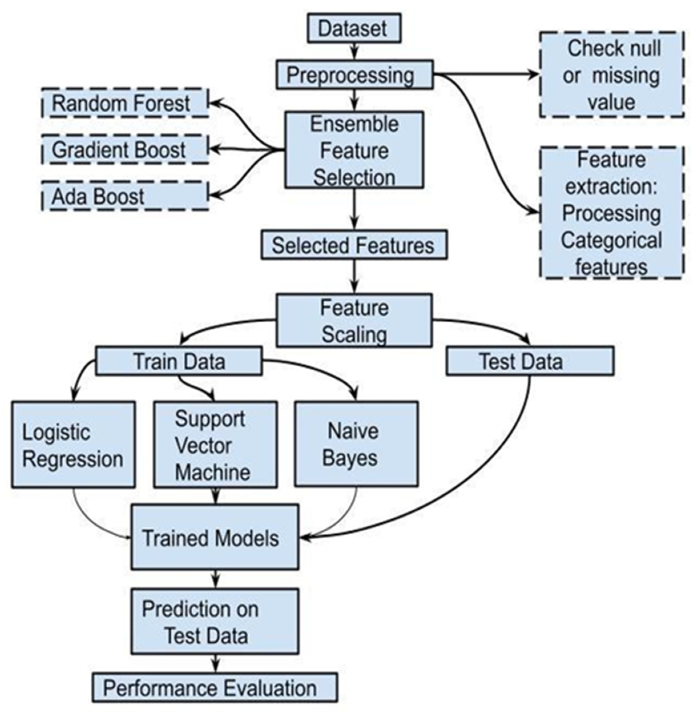
3.3.2. Proposed Model

In the secondary part of our model analysis, we aimed to improve the benchmark model and create a robust model for intrusion detection. A total of 27 models were created, where we used a varying number of feature selection techniques, features and machine learning algorithms for training. The workflow is shown in Figure 4.

Figure 4 showcases the process workflow for creating the 27 potential models. These models were a mathematical combination of three different ensemble feature selection techniques namely: random forest, gradient boosting machine and AdaBoost. Using these 3, different numbers of feature sets were selected, namely, 60 features, 30 features, 15 features, and 3 different machine learning algorithms for training, namely, logistic regression, support vector machine and naive Bayes models}.

As evident from Figure 4, we first loaded the dataset, which was followed by preprocessing, which included removing null values and performing feature extraction and dealing with categorical variables. After the preprocessing, the number of features increased from 41 to 121 features. The new feature set of 121 features consisted of 38 numerical features and 83 categorical features. The huge number of features now posed the problem of the curse of dimensionality [26]. Consequently, if dimensionality reduction had not been performed, it would have resulted in an increase in training time, computational power and difficulty for the machine learning algorithms to find robust relationships between dependent and independent variables. Keeping this in mind, we performed feature selection using 3 different ensemble techniques which selected 3 different sets of best features from our feature space of 121 features. We then scaled our data using a standard scaler [27], using the Scikit Learn library. These data were then fed to our 3 different machine learning algorithms for training and these trained models were then used to make predictions on the test data. Predictions were evaluated using various evaluation metrics. The quantitative results of the analysis for these 27 models are discussed in greater detail in the results section of the paper.

4. Results

In order to explain the results, this section aims to depict and present the results in greater detail and depth. The evaluation of results is divided into three phases: the baseline model evaluation, the optimal feature model evaluation and finally, the comparison of optimal feature models with the baseline model. To evaluate the performance of our feature selected models, three different evaluation metrics were used which are described briefly below:

• Elimination time: this describes the time taken by the ensemble algorithm to perform recursive feature elimination to get the set of most valuable features out of a total of 121 features available. This is largely important as a lower elimination time indicates a faster approach to identify the set of valuable features, but this metric alone does not provide conclusive evidence of the best technique to be used to build a robust intrusion detection system. Therefore, two other evaluation metrics, namely, accuracy and F1-score, were also used to identify the best model and comment on the accuracy and time trade-off of the models.
• Accuracy: for a binary classification problem, accuracy can be defined as the ratio of the sum of all true positives and true negatives to the sum of true positives, true negatives, false positive and false negative.
• F1-score: it is defined as the harmonic mean of precision and recall and is used to measure a test accuracy.

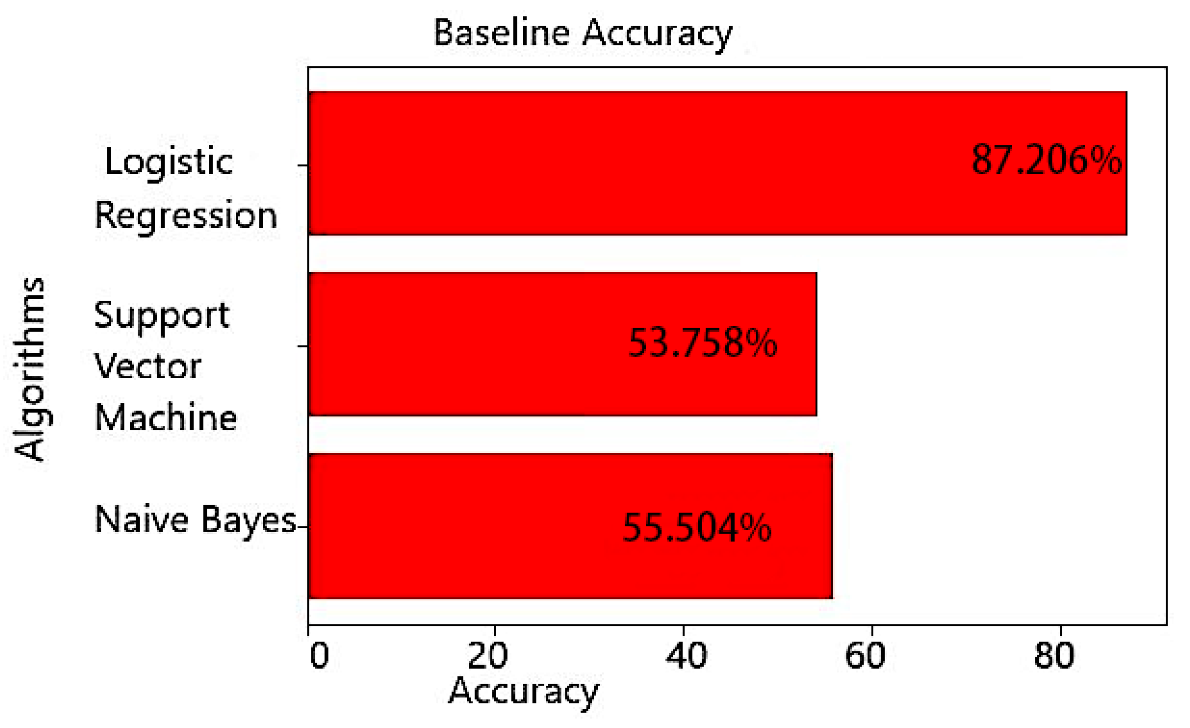
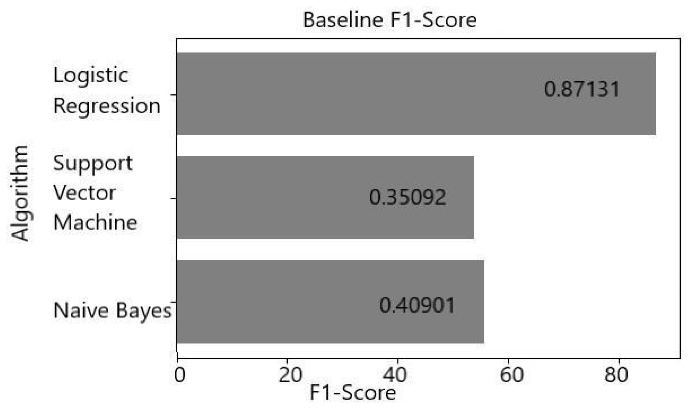
4.1. Evaluation of Baseline Model

We aimed to create a baseline model to build a reference point or benchmark to compare and analyse the results of our proposed techniques. In this subsection, we discuss the quantitative results pertaining to our approach for the baseline model shown in Figure 3.

From

Table 1. Accuracy and F1-score of baseline model.

Algorithm	Accuracy	F1-Score
Logistic regression	87.206%	0.87131
Support vector machine	53.758%	0.35092
Naive Bayes	55.504%	0.40901

, it is evident that the logistic regression model is best able to find the complex relationship between dependent and independent variables and achieves the highest accuracy and F1-score.

While creating the baseline model, no data preprocessing was performed and models were built using data which contained noise, thus making it particularly difficult to model the relationship between dependent and independent variables.

It is also evident from Figure 5 and Figure 6 that the logistic regression model is comparatively better than the support vector machine and naive Bayes as it achieves a higher accuracy and F1-score.

Therefore, the quantitative measures of performance, namely, accuracy and F1-score of our baseline model will now work as a benchmark or point of reference for next phases of our research.

4.2. Evaluation of 27 Feature Selected Model (Proposed)

In this subsection, the authors aim to holistically analyse the whole process of feature selection and the performance of the feature selection models using elimination time, accuracy and F1-score as evaluation metrics. This will largely help us to get an in-depth analysis of the whole process and will help us pinpoint the trade-offs and advantages of certain techniques over others.

For building feature selection models, we performed recursive feature elimination using the inbuilt Scikit Learn API. Three Ensemble algorithms namely random forest, gradient boosting and AdaBoost were used to perform recursive feature elimination. The process resulted in three sets of features containing 60, 30 and 20 features, respectively. The respective feature sets were then trained using logistic regression, support vector machines and naive Bayes. The quantitative results of the time it took to perform feature selection are shown in

Table 2. Time taken by ensemble feature selection algorithms.

No. of Features Selected	Random Forest	Gradient Boost	Ada Boost
60	21.009 s	133.8944 s	158.044 s
30	30.4625 s	183.720 s	222.788 s
20	36.819 s	190.019 s	234.9901 s

; the accuracy of the selected features is shown in

Table 3. Accuracy of 27 models (proposed) using various feature sets and feature selection techniques.

Algorithm	% Accuracy Using 60 Features			% Accuracy Using 30 Features			% Accuracy Using 20 Features
	RF	GB	AB	RF	GB	AB	RF	GB	AB
LR	97.04	97.02	97.01	96.77	96.69	96.77	94.09	95.58	96.53
SVM	98.86	98.86	98.87	99.08	99.06	98.94	98.43	98.77	98.58
NB	86.96	87.90	88.09	93.39	94.58	91.73	93.06	94.39	91.90

and the F1-score is shown in

Table 4. F1-Score of 27 models (proposed) using various feature set and feature selection techniques.

Algorithm	F1-Score Using 60 Features			F1-Score Using 30 Features			F1-Score Using 20 Features
	RF	GB	AB	RF	GB	AB	RF	GB	AB
LR	0.9703	0.9700	0.9699	0.9675	0.9667	0.9675	0.9406	0.9552	0.9651
SVM	0.9885	0.9885	0.9886	0.9908	0.9905	0.9893	0.9843	0.9876	0.9857
NB	0.8645	0.8747	0.8767	0.9338	0.9454	0.9172	0.9304	0.9434	0.9189

.

From Table 2, we can see that the elimination time of the random forest algorithm for finding the best possible set of features is minimum in the three cases where we aimed to find out the best 60, best 30 and best 20 features from our feature set of 121 features.

Though the elimination time of the random forest algorithm might be the least when compared to the other two algorithms, that does not necessarily mean that the set of features the random forest (RF) was able to find in the three cases are the best for modelling our problem. Therefore, to reach conclusive evidence about which algorithm was able to find the best set of features for the cases we further needed to look into the performance of the machine learning algorithms which used those sets of features for testing and making predictions on the test data.

From Table 3 and Table 4, we can clearly see that AdaBoost (AB) was the best feature selection technique to identify the most valuable set of 60 features, having the highest accuracy and F1-score when used with a support vector machine as the classifier.

Gradient boost (GB) as a feature selection technique was best able to select a set of 20 features to model the relationship between dependent and independent variables using a support vector machine.

However, from Table 3 and Table 4, it is evident that the combination of random forest for feature selection and support vector machine for training the classifier gave the highest accuracy and F1-score on the test data using only 30 features, when compared to other combinations of feature selection and training algorithms with varying number of features in the feature set. It can also be concluded from Table 4 that random forest has a comparatively lesser feature selection time compared to the other ensemble techniques hence making it a robust and time efficient technique.

Furthermore, Table 3 and Table 4 suggest that a set of 30 features is the optimal number of features for our particular problem as both increase to 60 features or decrease to 20 features caused a degradation in the accuracy and F1-score of our models.

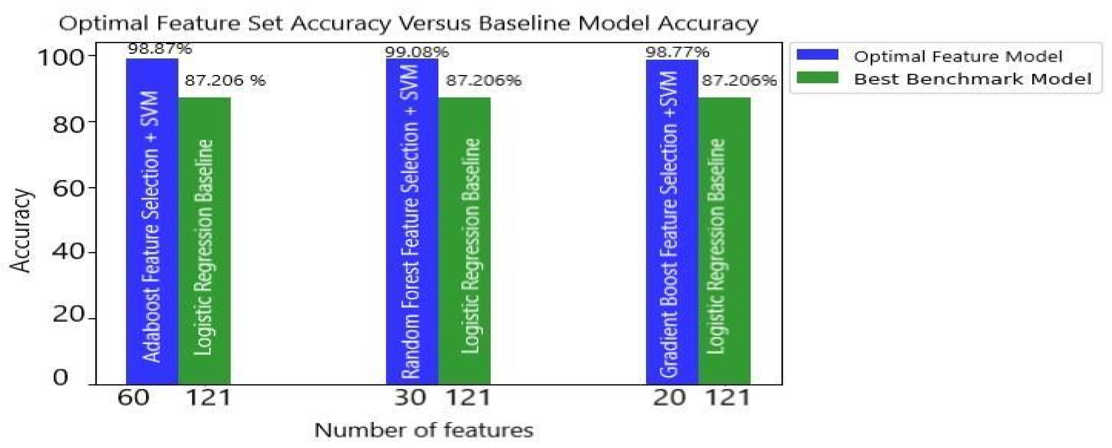
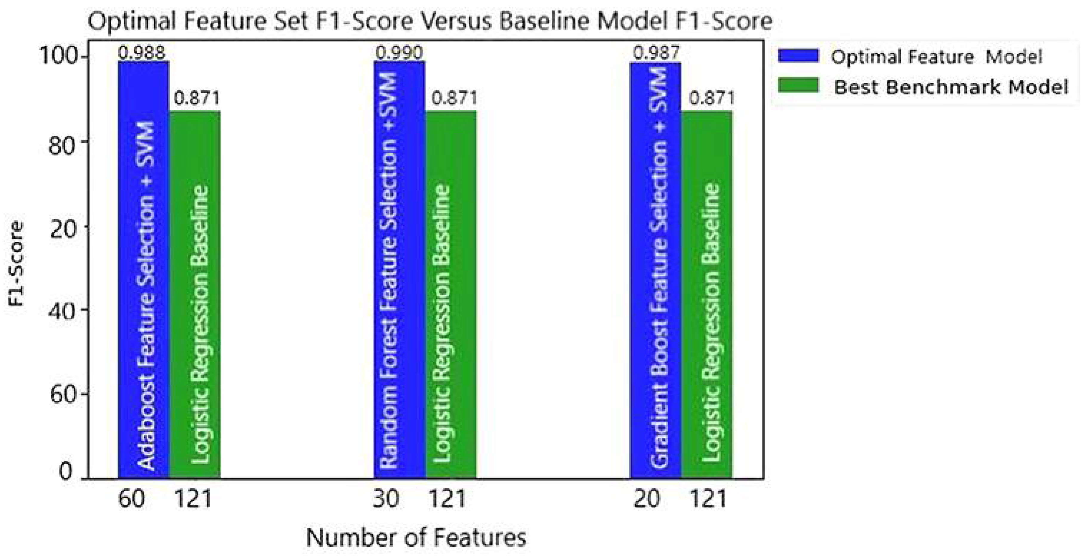
4.3. Comparison of Optimal Feature Model with Baseline Model

In the last two subsections we show how the baseline model and machine learning models with optimal feature sets were modelled. In this subsection, the authors quantitatively analyse the improvements in performance of those machine learning models generated by the optimal feature sets compared to the baseline model [28,29]. The visual differences in accuracy and F1-score can be seen in the bar graph in Figure 7 and Figure 8.

Figure 7 shows the highest accuracy achieved by the combination of various feature selection and machine learning techniques for a varying feature set containing 60, 30 or 20 features. It also shows that each of our optimal feature models with a lesser number of features compared to our baseline model outperformed the performance of our baseline model, which had an accuracy of 87.206%.

Similar inferences can be made from Figure 8, which shows the highest F1-score achieved by the combination of various feature selection and machine learning techniques for a varying feature set containing 60, 30 or 20 features

5. Discussion

The proposed optimal feature models have a lesser number of features compared to our baseline model and outperformed the performance of our baseline model which had a F1-score of 0.871.

Table 5. Comparison of optimal feature set models with baseline model.

Model	(%) Accuracy	F1-Score	Accuracy Increment	F1-Score Increment	Features Used (%)
LR Baseline (121 Features)	87.20	0.871	-	-	-
AB + SVM (60 Features)	98.87	0.988	11.664	0.117	49.58
RF + SVM (30 Features)	99.08	0.990	11.874	0.119	24.79
GB + SVM (20 Features)	98.77	0.987	11.564	0.116	16.52

depicts quantitatively the improvement made by our research when compared with the baseline model.

From Table 5, we can see the accuracy and F1-score increment in our optimal feature models when compared to the baseline model. This experimentation found that the combination of a random forest for feature selection and a support vector machine for training our model on those selected features provides the highest accuracy and F1-score increment. Moreover, it was found that the optimal number of features for our problem was 30 features as increment or decrement in feature count reduced the accuracy of our models. The results discussed above have some major overlapping drawbacks as the model is not fully capable of identifying zero-day attack, the performance of the model is also very dependent on the train-test data distribution and how the hyperparameters are tuned.

Pertaining to these results, it can be inferred that integrating artificial intelligence into intrusion detection systems (IDSs) will largely help industry and organisations, as they will not have to depend on rule-based systems to identify potential threats to the system, and any new signatures classified as threats may be added to the database for future analysis and detection. This will automate the workflow of identifying threats and reduce the manual intervention required to perform such detection, which is also prone to manual error at times.

6. Conclusions

This paper primarily focused on improving the performance of intrusion detection systems. It first created a benchmark/baseline model, which was later enhanced by using three different ensemble feature selection techniques combined with three machine learning algorithms. A comparative analysis of feature selection techniques was presented using elimination time as the metric. This comparative analysis using machine learning models was performed using accuracy and F1-score as the performance metrics. It was observed that the proposed approach of a random forest with a support vector machine outperformed all other 26 models as reported in Discussion Section. The results indicated an improvement of 11.874% in absolute accuracy and 0.119 in terms of absolute F1-Score as compared to the existing model using logistic regression from the literature. This proposed model also satisfied the requirements of having a low latency and high predictive accuracy. In the future, to further work on reducing the latency of the systems, various feature selection techniques such as filter-based feature selection, simulated annealing can be investigated with deep learning and hybrid deep learning models. This proposed model can also be effectively used in real-time systems, which process millions of gigabytes of data thanks to the advancement in network technology as a future perspective.

References

1. Internet Growth Statistics 1995 to 2021—The Global Village Online. Available online: https://www.internetworldstats.com/emarketing.htm (accessed on 13 September 2021).
2. Nobakht, M.; Sivaraman, V.; Boreli, R. A host-based intrusion detection and mitigation framework for smart home iot using openflow. In Proceedings of the 2016 11th International Conference on Availability, Reliability and Security (ARES), Salzburg, Austria, 31 August–2 September 2016; IEEE: New York, NY, USA, 2016; pp. 147–156. [Google Scholar]
3. Vailshery, L.S. Number of Connected Devices Worldwide 2030 (January 2021). Available online: https://www.statista.com/ (accessed on 16 September 2021).
4. Perwej, Y.; Haq, K.; Parwej, F.; Mumdouh, M.; Hassan, M. The internet of things (iot) and its application domains. Int. J. Comput. Appl. 2019, 975, 182. [Google Scholar] [CrossRef]
5. Theodoridis, E.; Mylonas, G.; Chatzigiannakis, I. Developing an iot smart city framework. In Proceedings of the IISA 2013, Piraeus, Greece, 10–12 July 2013; IEEE: New York, NY, USA, 2013; pp. 1–6. [Google Scholar]
6. Liao, H.J.; Lin, C.H.R.; Lin, Y.C.; Tung, K.Y. Intrusion detection system: A comprehensive review. J. Netw. Comput. Appl. 2013, 36, 16–24. [Google Scholar] [CrossRef]
7. Lastdrager, E.E. Achieving a consensual definition of phishing based on a systematic review of the literature. Crime Sci. 2014, 3, 9. [Google Scholar] [CrossRef]
8. Zaharia, A. 300+ Terrifying Cybercrime & Cybersecurity Statistics [2021 Edition] (March 2021). Available online: https://www.comparitech.com (accessed on 16 September 2021).
9. Phishing Activity Trends Reports. Available online: https://apwg.org/trendsreports/ (accessed on 18 September 2021).
10. Netscout Threat Intelligence Report (April 2021). Available online: https://www.netscout.com/threatreport365 (accessed on 21 September 2021).
11. Finkelhor, D.; Walsh, K.; Jones, L.; Mitchell, K.; Collier, A. Youth internet safety education: Aligning programs with the evidence base. Trauma Violence Abuse 2020, 22, 1233–1247. [Google Scholar] [CrossRef] [PubMed]
12. Anand, A.; Patel, B. An overview on intrusion detection system and types of attacks it can detect considering different protocols. Int. J. Adv. Res. Comput. Sci. Softw. Eng. 2012, 2, 94–98. [Google Scholar]
13. Pedregosa, F.; Varoquaux, G.; Gramfort, A.; Michel, V.; Thirion, B.; Grisel, O.; Blondel, M.; Prettenhofer, P.; Weiss, R.; Dubourg, V.; et al. Scikit-learn: Machine learning in Python. J. Mach. Learn. Res. 2011, 12, 2825–2830. [Google Scholar]
14. Alkasassbeh, M.; Almseidin, M. Machine learning methods for network intrusion detection. arXiv 2018, arXiv:1809.02610. [Google Scholar]
15. Choudhury, S.; Bhowal, A. Comparative analysis of machine learning algorithms along with classifiers for network intrusion detection. In Proceedings of the 2015 International Conference on Smart Technologies and Management for Computing, Communication, Controls, Energy and Materials (ICSTM), Chennai, India, 6–8 May 2015; IEEE: New York, NY, USA, 2015; pp. 89–95. [Google Scholar]
16. Belouch, M.; El Hadaj, S.; Idhammad, M. Performance evaluation of in trusion detection based on machine learning using Apache Spark. Proc. Comput. Sci. 2018, 127, 1–6. [Google Scholar] [CrossRef]
17. Koc, L.; Mazzuchi, T.A.; Sarkani, S. A network intrusion detection system based on a hidden naïve bayes multiclass classifier. Exp. Syst. Appl. 2012, 39, 13492–13500. [Google Scholar] [CrossRef]
18. Tang, T.A.; Mhamdi, L.; McLernon, D.; Zaidi, S.A.R.; Ghogho, M. Deep learning approach for network intrusion detection in software defined networking. In Proceedings of the 2016 International Conference on Wireless Networks and Mobile Communications (WINCOM), Reims, France, 27–29 October 2020; IEEE: New York, NY, USA, 2016; pp. 258–263. [Google Scholar]
19. Prabakar, D.; Sasikala, S.; Saravanan, T.; Gomathi, S.; Ramesh, S. Enhanced simulating an nealing and svm for intrusion detection system in wireless sensor networks. Res. Sq. 2021. [Google Scholar] [CrossRef]
20. Rajagopal, S.; Kundapur, P.P.; Hareesha, K.S. A stacking ensemble for network intrusion detection using heterogeneous datasets. Secur. Commun. Netw. 2020, 2020, 4586875. [Google Scholar] [CrossRef] [Green Version]
21. Ambwani, T. Multi class support vector machine implementation to intru395 sion detection. In Proceedings of the IEEE International Joint Conference on Neural Networks, Portland, OR, USA, 20–24 July 2003; Volume 3, pp. 2300–2305. [Google Scholar]
22. Bhosale, S. Network Intrusion Detection (October 2018). Available online: https://www.kaggle.com/sampadab17 (accessed on 19 July 2021).
23. Sperandei, S. Understanding logistic regression analysis. Biochem. Med. 2014, 24, 12–18. [Google Scholar] [CrossRef] [PubMed]
24. Cox, D.R. The regression analysis of binary sequences. J. R. Stat. Soc. Ser. B 1958, 20, 215–232. [Google Scholar] [CrossRef]
25. Vapnik, V. Pattern recognition using generalized portrait method. Automat. Remote Control 1963, 24, 774–780. [Google Scholar]
26. Murphy, K.P. Machine Learning: A Probabilistic Perspective; MIT Press: Cambridge, MA, USA, 2012. [Google Scholar]
27. Sharma, U.; Tomar, P.; Ali, S.S.; Saxena, N.; Bhadoria, R.S. Optimized authentication system with high security and privacy. Electronics 2021, 10, 458. [Google Scholar] [CrossRef]
28. Swarnkar, M.; Bhadoria, R.S.; Sharma, N. Security, privacy, trust management and performance optimization of blockchain technology. In Applications of Blockchain in Healthcare; Springer: Singapore, 2021; pp. 69–92. [Google Scholar]
29. Sharma, P.; Borah, M.D.; Namasudra, S. Improving security of medical big data by using Blockchain technology. Comput. Electr. Eng. 2021, 96, 107529. [Google Scholar] [CrossRef]
Figure 1. High-level architecture of intrusion detection system (IDS).
Applsci 11 11988 g001
Figure 2. Number instances of each class in normal and anomaly datasets.
Applsci 11 11988 g002
Figure 3. Workflow for creating baseline model.
Applsci 11 11988 g003
Figure 4. Workflow for creating 27 experimental models.
Applsci 11 11988 g004
Figure 5. Accuracy of baseline models.
Applsci 11 11988 g005
Figure 6. F1-score of baseline models.
Applsci 11 11988 g006
Figure 7. Accuracy comparison of optimal feature set model and baseline model.
Applsci 11 11988 g007
Figure 8. F1-score comparison of optimal feature set model and baseline model.
Applsci 11 11988 g008