Modeling and Stability Analysis for the Vibrating Motion of Three Degrees-of-Freedom Dynamical System Near Resonance

Abstract

The focus of this article is on the investigation of a dynamical system consisting of a linear damped transverse tuned-absorber connected with a non-linear damped-spring-pendulum, in which its hanged point moves in an elliptic path. The regulating system of motion is derived using Lagrange’s equations, which is then solved analytically up to the third approximation employing the approach of multiple scales (AMS). The emerging cases of resonance are categorized according to the solvability requirements wherein the modulation equations (ME) have been found. The stability areas and the instability ones are examined utilizing the Routh–Hurwitz criteria (RHC) and analyzed in line with the solutions at the steady state. The obtained results, resonance responses, and stability regions are addressed and graphically depicted to explore the positive influence of the various inputs of the physical parameters on the rheological behavior of the inspected system. The significance of the present work stems from its numerous applications in theoretical physics and engineering.

1. Introduction

In the last two decades, some researchers have produced numerous works trying to solve the problems of excessive vibrations of mechanical systems, including the use of absorbers to treat and absorb active and the passive vibrations, e.g., [1,2,3,4,5,6].

The motion of a pendulum vibration absorber (PVA) with a spin base is investigated in [2] to deal with vertical excitation. By altering the rotational motion, the distinctive frequency of the pendulum absorber can be modified dynamically over a large range. A longitudinal absorber is used in [3] to stabilize and regulate vibrations of a spring pendulum, with non-linear stiffness, expressing ship roll motion. To achieve a semi-closed solution for the approximation from second order, the authors used the approach of multiple scales (AMS) [7], investigating the response of the considered model near resonance cases. They applied the influence of an additional transvers absorber to generalize this problem as in [4] and [5]. It is demonstrated in [6] how to autonomously modify the rotating speed of PVA, with two degrees of freedom (DOF), by identifying the phase between the PVA and primary vibrations. The pivot’s motion of a simple pendulum with rigid arm that connected with a longitudinal absorber on an elliptic trajectory is examined in [8]. All resonance cases are generally grouped, and the case of two concurrent basic external resonances is examined. The generalization of this work is found in [9] for the case of a damped elastic pendulum instead of the un-stretched one. The ME are obtained and solved numerically to check the stability and instability regions in view of RHC.

Different trajectories for a pivot point of linear and non-linear elastic pendulums with various DOF are studied in numerous works, e.g., [10,11,12,13,14,15,16,17,18,19]. The case of fixed pivot point of 3DOF rigid body pendulum (RBP) is examined in [10], in which three resonance cases are studied simultaneously from the perspective of the AMS. In [11,12], the authors dealt with a damped pendulum motion under the influence of various forces taking into account the movement of the pivot point on a circle with a stationary angular velocity. In [13,14,15], Lissajous paths are considered for the motion of the spring’s suspension point as constrained motion. All possible fixed points are graphed in [13] and categorized in terms of being stable or not, while in [14], the authors verified the obtained analytic solutions for the elastic RBP through comparison with the numerical results. The approximate solutions and their stability regions for a non-linear damped RBP are examined in [15] using the AMS and RHC, respectively.

Many scientific works have recently studied the motion of the pendulum’s suspension point on elliptic pathways for a variety of models such as [16,17,18,19]. The linear and non-linear dampings of a spring RBP on an elliptic route are inspected in [16,17], respectively. The double pendulum motion on an elliptic pathway was studied in [18]; one of them is a simple rigid pendulum while the other one is an elastically damped. The motion was investigated when a longitudinal harmonic force and a rotating moment were applied to the pendulum end point and to the suspension point, respectively. The effect of two external perpendicular forces besides an applied moment on a spring pendulum motion movement that follows the same route is examined in [19].

Two systems were considered in [20]: the first one is a subsystem that produces a swing motion, and the other is an absorber that moves linearly with respect to it, which can be used in various fields of engineering. The harmonic balance method (HBM) [7] is applied in [21] to examine the vibrational response of a connected mass with a damped oscillator, in addition to an excited pendulum hinged to this mass. The averaging approach is employed in [22] to obtain the analytic results of the 2DOF non-linear vibrating dynamical system consisting of a non-linear spring with attached damper. The authors concluded that the oscillation and amplitude can be reduced through adjusting the parameters of the system. Therefore, it can be used to improve the design of a non-linear absorber. The vibrating motion of an auto-parametric absorber (APA) connected with a Duffing oscillator was investigated numerically and experimentally in [23]. The impacts of a magneto-rheological (MR) damper and a shape storage alloy (SMA) spring on the absorption effect and regular solution stability were investigated in [24], while the author presented in [25] an analysis of the oscillation and energy harvesting of APA vibration. The analytical, computational, and experimental studies of a dynamical system containing an electromagnetic device are presented in [26], in which the analytic solutions were achieved using the HBM. Therefore, the author constructed another dynamic model in [27] to reduce the vibration and harvesting energy simultaneously, in which it is concluded that the initial resonance’s area is the ideal area for suppression. The presence of solutions for a class of multi-point boundary value problems presented on the positive half-line for a fractional differential equation at resonance is explored in [28]. The asymptotic behavior of dynamical system trajectories caused by the algorithm and generalized known results when the metric space is bounded are examined in [29].

This study addresses the behavior of a 3DOF vibrating system consisting of a non-linear damped spring pendulum linked to an absorber with linear damper, which is exposed to the impact of a force in the spring’s transverse direction. It is assumed that the whole motion is in a plane in which the spring’s hanging point rotates in an elliptic path with steady angular velocity. The second kind of Lagrange’s equations have been used to construct the equations of motion (EOM), which are then solved using the AMS up to the third approximations. The requirements of solvability were satisfied through the elimination of secular terms, and thereby, the ME were gained. The RHC was used to examine the fixed points of the stability analysis of solutions at the steady state. As a result, the non-linear stability was examined to determine the zones of stability and instability. The system’s behavior is depicted through the examination of several plots relating to various curves of the solutions’ time histories, resonance, and stability zones. This model is significant since it is used in a variety of engineering applications such as construction, bridges, and spinning machines.

2. Description of the Vibrating System

A vibrational system with 3DOF is described in Figure 1, in which a damped elastic pendulum with normal length $l_0$, non-linear stiffness $K_1$ and $K_2$, and pendulum mass $m_1$ is considered. A pivot point $O_1$ of the pendulum is limited to move in an elliptic route with stationary angular velocity $\mathrm{\Omega }$, while the pendulum’s other end is attached to a linear absorber of mass $m_2$, a normal length $l_{10}$, and linear stiffness $K_3$. According to the sketch of Figure 1, we may write the corresponding coordinates of $O_1$ to the axes $OX$ and $OY$ in the forms $a\cos (\mathrm{\Omega }t)$ and $b\sin (\mathrm{\Omega }t)$, respectively. Here, the ellipse’s minor and major axes are represented by $a$ and $b$, respectively. On the supplementary circle $b$, the equivalent point of $O_1$ will be assigned by $Q$.

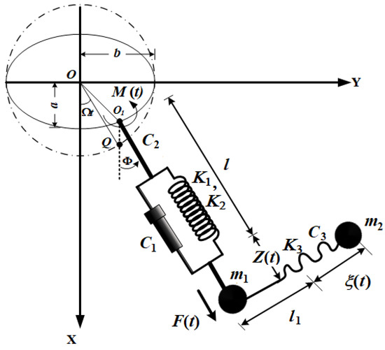
Figure 1. The examined model.

The system’s motion is addressed to be under the influence of applied harmonic force $F(t)=F_1\cos ({\mathrm{\Omega }}_{1}t)$ at the spring’s radial direction, as well as a harmonic moment $M(t)=M_0\cos ({\mathrm{\Omega }}_{2}t)$ at $O_1$ in the anticlockwise direction. Here, ${\mathrm{\Omega }}_1,{\mathrm{\Omega }}_2$ and $F_1,M_0$ are the frequencies and amplitudes of $F(t)$ and $M(t)$. The extensions of the spring and absorber are supposed to be $Z(t)$ and $\xi (t)$, respectively. Furthermore, $C_1,C_2,$ and $C_3$ are thought to indicate the coefficients of viscous damping for the spring’s longitudinal, swing oscillations, and the absorber’s elongation, respectively.

The kinetic and potential energies $T$ and $V$ of the system can be expressed in the following ways

$$\begin{array}{ll}T& =\frac{1}{2}(m_1+m_2)\{{\mathrm{\Omega }}^2[a^2{\sin }^2(\mathrm{\Omega }t)+b^2{\cos }^2(\mathrm{\Omega }t)]+{Z^{\prime }}^2+{(l+Z)}^2{{\mathrm{\Phi }}^{\prime }}^2\\ & +2\mathrm{\Omega }{Z}^{\prime }[b\cos (\mathrm{\Omega }t)\sin \mathrm{\Phi }-a\sin (\mathrm{\Omega }t)\cos \mathrm{\Phi }]+2\mathrm{\Omega }(l+Z){\mathrm{\Phi }}^{\prime }\\ & \times [b\cos (\mathrm{\Omega }t)\cos \mathrm{\Phi }+a\sin (\mathrm{\Omega }t)\sin \mathrm{\Phi }]\}+\frac{1}{2}{m}_2\{{{\xi }^{\prime }}^2+{(l_1+\xi )}^2{{\mathrm{\Phi }}^{\prime }}^2\\ & -2\mathrm{\Omega }(l_1+\xi ){\mathrm{\Phi }}^{\prime }[b\cos (\mathrm{\Omega }t)\sin \mathrm{\Phi }+a\sin (\mathrm{\Omega }t)\cos \mathrm{\Phi }]+2\mathrm{\Omega }{\xi }^{\prime }\\ & \times [b\cos (\mathrm{\Omega }t)\cos \mathrm{\Phi }-a\sin (\mathrm{\Omega }t)\sin \mathrm{\Phi }]+2Z^{\prime }{\xi }^{\prime }\sin (2\mathrm{\Phi })+2(l_1+\xi )\\ & \times Z^{\prime }{\mathrm{\Phi }}^{\prime }\cos (2\mathrm{\Phi })+2(l+Z){\mathrm{\Phi }}^{\prime }{\xi }^{\prime }\cos (2\mathrm{\Phi })-2(l+Z)(l_1+\xi ){{\mathrm{\Phi }}^{\prime }}^2\sin (2\mathrm{\Phi })\},\\ V& =\frac{1}{2}{K}_1{(Z+Z_r)}^2+\frac{1}{3}{K}_2{(Z+Z_r)}^3+\frac{1}{2}{K}_3{(\xi +{\xi }_r)}^2+m_{1}g(l+Z)(1-\cos \mathrm{\Phi })\\ & +m_{2}g[(l+Z)(1-\cos \mathrm{\Phi })+(l_1+\xi )\sin \mathrm{\Phi }];\\ l& =l_0+Z_r,\hspace{0.17em}\hspace{0.17em}\hspace{0.17em}\hspace{0.17em}\hspace{0.17em}\hspace{0.17em}\hspace{0.17em}{l}_1=l_{10}+{\xi }_r.\end{array}$$

(1)

Here, $Z_r$ and ${\xi }_r$ are the spring’s and the absorber’s static elongations, respectively; the angle formed by the vertical at $O_1$ and the line passing across $O_1{m}_1$ are denoted by $\mathrm{\Phi }$; $g$ is the acceleration of gravity, and the primes are the differentiation in relation to time $t$.

According to Equation (1), Lagrange’s function $L=T-V$ can be determined, and then, the controlling system of motion can be obtained using the next equations of Lagrange [30]

$$\begin{array}{l}\frac{d}{dt}(\frac{\partial L}{\partial Z^{\prime }})-\frac{\partial L}{\partial Z}=Q_Z,\\ \frac{d}{dt}(\frac{\partial L}{\partial {\mathrm{\Phi }}^{\prime }})-\frac{\partial L}{\partial \mathrm{\Phi }}=Q_{\mathrm{\Phi }},\\ \frac{d}{dt}(\frac{\partial L}{\partial {\xi }^{\prime }})-\frac{\partial L}{\partial \xi }=Q_{\xi }.\end{array}$$

(2)

Here, $(Q_Z,Q_{\mathrm{\Phi }},Q_{\xi })$ are the system’s non-conservative generalized forces, while $(Z,\mathrm{\Phi },\xi )$ and $(Z^{\prime },{\mathrm{\Phi }}^{\prime },{\xi }^{\prime })$ are the generalized coordinates and velocities, respectively. The forms of $Q_Z,Q_{\mathrm{\Phi }},$ and $Q_{\xi }$ are

$$\begin{array}{l}{Q}_Z=F_1\cos ({\mathrm{\Omega }}_{1}t)-C_1{Z}^{\prime },\\ Q_{\mathrm{\Phi }}=M_0\cos ({\mathrm{\Omega }}_{2}t)-C_2{\mathrm{\Phi }}^{\prime },\\ Q_{\xi }=-C_3{\xi }^{\prime }.\end{array}$$

(3)

Substituting from (1) and (3) into (2), the dimensionless form of the controlling system of EOM has the following form

$$\begin{array}{cc}\hfill \ddot{z}+c_1\dot{z}& +z+z_r+\alpha {(z+z_r)}^2+(1-\cos \mathrm{\Phi })w_1^2-(1+z){\dot{\mathrm{\Phi }}}^2+\beta [(\ddot{\eta }-(r+\eta ){\dot{\mathrm{\Phi }}}^2)\hfill \\ & \times \sin (2\mathrm{\Phi })+((r+\eta )\ddot{\mathrm{\Phi }}+2\dot{\mathrm{\Phi }}\dot{\eta })\cos (2\mathrm{\Phi })]-\frac{{\varpi }^2}{l}[b\sin (\varpi \tau )\sin \mathrm{\Phi }\hfill \\ & +a\cos (\varpi \tau )\cos \mathrm{\Phi }]=f_{1}cos(p_1\tau ),\hfill \\ \hfill \{{(1+z)}^2& +\beta [{(r+\eta )}^2-2(1+z)(r+\eta )\sin (2\mathrm{\Phi })]\}\ddot{\mathrm{\Phi }}+c_2\dot{\mathrm{\Phi }}+2[1+z\hfill \\ & -2\beta (r+\eta )\sin (2\mathrm{\Phi })]\dot{z}\hspace{0.17em}\dot{\mathrm{\Phi }}+2[(r+\eta )-(1+z)\sin (2\mathrm{\Phi })]\beta \hspace{0.17em}\dot{\mathrm{\Phi }}\hspace{0.17em}\dot{\eta }\hfill \\ & +(1+z)w_1{}^2\sin \mathrm{\Phi }+\beta (r+\eta )w_1{}^2\cos \mathrm{\Phi }+\beta [(r+\eta )\ddot{z}+(1+z)\ddot{\eta }\hfill \\ & -2(r+\eta )(1+z){\dot{\mathrm{\Phi }}}^2]\cos (2\mathrm{\Phi })-\frac{{\varpi }^2}{l}(1+z)[b\sin (\varpi \tau )\cos \mathrm{\Phi }-a\cos (\varpi \tau )\hfill \\ & \times \sin \mathrm{\Phi }]+\frac{{\varpi }^2}{l}\beta (r+\eta )[b\sin (\varpi \tau )\sin \mathrm{\Phi }-a\cos (\varpi \tau )\cos \mathrm{\Phi }]=m_0\cos (p_2\tau ),\hfill \\ \hfill \ddot{\eta }+\ddot{z}\sin (2\mathrm{\Phi })& +c_3\dot{\eta }-\frac{{\varpi }^2}{l}[b\sin (\varpi \tau )\cos \mathrm{\Phi }+a\cos (\varpi \tau )\sin \mathrm{\Phi }]-[(1+z)\sin (2\mathrm{\Phi }\hspace{0.17em})\hfill \\ & +r+\eta ]{\dot{\mathrm{\Phi }}}^2+[2\dot{z}\hspace{0.17em}\dot{\mathrm{\Phi }}+(1+z)\ddot{\mathrm{\Phi }}]\cos (2\mathrm{\Phi })+w_1^2\sin \mathrm{\Phi }+w_2^2(\eta +{\eta }_r)=0,\hfill \end{array}$$

(4)

where

$$\begin{array}{l}\tau ={\omega }_{1}t,\hspace{0.17em}\hspace{0.17em}\hspace{0.17em}\hspace{0.17em}z=\frac{Z}{l},\hspace{0.17em}\hspace{0.17em}\hspace{0.17em}\hspace{0.17em}{z}_r=\frac{Z_r}{l},\hspace{0.17em}\hspace{0.17em}\hspace{0.17em}\hspace{0.17em}\eta =\frac{\xi }{l},\hspace{0.17em}\hspace{0.17em}\hspace{0.17em}\hspace{0.17em}{\eta }_r=\frac{{\xi }_r}{l},\hspace{0.17em}\hspace{0.17em}\hspace{0.17em}\hspace{0.17em}{\omega }_1=\sqrt{\frac{K_1}{m_1+m_2}},\hspace{0.17em}\hspace{0.17em}\hspace{0.17em}\hspace{0.17em}{\omega }_2=\sqrt{\frac{g}{l}},\\ {\omega }_3=\sqrt{\frac{K_3}{m_2}},\hspace{0.17em}\hspace{0.17em}\hspace{0.17em}\hspace{0.17em}{w}_1=\frac{{\omega }_2}{{\omega }_1},\hspace{0.17em}\hspace{0.17em}\hspace{0.17em}\hspace{0.17em}{w}_2=\frac{{\omega }_3}{{\omega }_1},\hspace{0.17em}\hspace{0.17em}\hspace{0.17em}\hspace{0.17em}\varpi =\frac{\mathrm{\Omega }}{{\omega }_1},\hspace{0.17em}\hspace{0.17em}\hspace{0.17em}\hspace{0.17em}\beta =\frac{m_2}{m_1+m_2},\hspace{0.17em}\hspace{0.17em}\hspace{0.17em}\hspace{0.17em}r=\frac{l_1}{l},\\ \alpha =\frac{K_{2}l}{{\omega }_1^2(m_1+m_2)},\hspace{0.17em}\hspace{0.17em}\hspace{0.17em}\hspace{0.17em}{c}_1\hspace{0.17em}=\frac{C_1}{(m_1+m_2){\omega }_1},\hspace{0.17em}\hspace{0.17em}\hspace{0.17em}\hspace{0.17em}{c}_2=\frac{C_2}{(m_1+m_2)l^2{\omega }_1},\hspace{0.17em}\hspace{0.17em}\hspace{0.17em}\hspace{0.17em}{c}_3=\frac{C_3}{m_2{\omega }_1},\\ f_1=\frac{F_1}{(m_1+m_2)l{\omega }_1^2},\hspace{0.17em}\hspace{0.17em}\hspace{0.17em}\hspace{0.17em}{m}_0=\frac{M_0}{(m_1+m_2)l^2{\omega }_1^2},\hspace{0.17em}\hspace{0.17em}\hspace{0.17em}\hspace{0.17em}{p}_1=\frac{{\mathrm{\Omega }}_1}{{\omega }_1},\hspace{0.17em}\hspace{0.17em}\hspace{0.17em}\hspace{0.17em}{p}_2=\frac{{\mathrm{\Omega }}_2}{{\omega }_1},\end{array}$$

Denote the parameters that are dimensionless, and the dots represent the differentiation regarding to $\tau$, in which the generalized coordinates and their corresponding first derivatives have the following initial conditions

$$\begin{array}{l}z(0)=z_0,\hspace{0.17em}\hspace{0.17em}\hspace{0.17em}\hspace{0.17em}\hspace{0.17em}\hspace{0.17em}\mathrm{\Phi }(0)={\mathrm{\Phi }}_0,\hspace{0.17em}\hspace{0.17em}\hspace{0.17em}\hspace{0.17em}\hspace{0.17em}\hspace{0.17em}\eta (0)={\eta }_0,\\ \dot{z}(0)=0,\hspace{0.17em}\hspace{0.17em}\hspace{0.17em}\hspace{0.17em}\hspace{0.17em}\hspace{0.17em}\hspace{0.17em}\dot{\mathrm{\Phi }}(0)=0,\hspace{0.17em}\hspace{0.17em}\hspace{0.17em}\hspace{0.17em}\hspace{0.17em}\hspace{0.17em}\hspace{0.17em}\hspace{0.17em}\hspace{0.17em}\hspace{0.17em}\dot{\eta }(0)=0.\end{array}$$

3. The Desired Solutions

In this part of the present research work, we use the AMS to acquire the approximate analytic solutions of the EOM (4), categorize the different cases of resonance, and extract both the solvability criteria and the ME. Then, we look at the oscillations of the system close to the static equilibrium position [31]. To accomplish this target, we approximate the functions $\sin \mathrm{\Phi }$ and $\cos \mathrm{\Phi }$ up to the third-order as follows

$$\sin \mathrm{\Phi }=\mathrm{\Phi }-\frac{{\mathrm{\Phi }}^3}{6}, \hspace{0.17em}\hspace{0.17em}\hspace{0.17em}\hspace{0.17em}\hspace{0.17em}\hspace{0.17em}\hspace{0.17em}\hspace{0.17em}\hspace{0.17em}\hspace{0.17em}\hspace{0.17em}\hspace{0.17em}\hspace{0.17em}\hspace{0.17em}\hspace{0.17em}\hspace{0.17em}\cos \mathrm{\Phi }=1-\frac{{\mathrm{\Phi }}^2}{2}.$$

(5)

The damping coefficients, force’s amplitudes, moment, elliptical semi-axes, and other parameters can then be represented in terms of a small parameter $0<\epsilon <<1$ as follows

$$\begin{array}{l}{c}_1={\epsilon }^2{\tilde{c}}_1,\hspace{0.17em}\hspace{0.17em}\hspace{0.17em}\hspace{0.17em}{c}_2={\epsilon }^2{\tilde{c}}_2,\hspace{0.17em}\hspace{0.17em}\hspace{0.17em}\hspace{0.17em}{c}_3={\epsilon }^2{\tilde{c}}_3,\hspace{0.17em}\hspace{0.17em}\hspace{0.17em}\hspace{0.17em}\beta =\epsilon \tilde{\beta },\hspace{0.17em}\hspace{0.17em}\hspace{0.17em}\hspace{0.17em}\\ f_1={\epsilon }^3{\tilde{f}}_1,\hspace{0.17em}\hspace{0.17em}\hspace{0.17em}\hspace{0.17em}{m}_0={\epsilon }^3{\tilde{m}}_0,\hspace{0.17em}\hspace{0.17em}\hspace{0.17em}\hspace{0.17em}a={\epsilon }^2\tilde{a},\hspace{0.17em}\hspace{0.17em}\hspace{0.17em}\hspace{0.17em}b={\epsilon }^2\tilde{b},\hspace{0.17em}\hspace{0.17em}\hspace{0.17em}\hspace{0.17em}\alpha ={\epsilon }^2\tilde{\alpha }.\end{array}$$

(6)

As a result, we can express the functions $z,\mathrm{\Phi },$ and $\eta$ in terms of $\epsilon$ and the new functions $\tilde{z},\tilde{\mathrm{\Phi }},$ and $\tilde{\eta }$ as follows

$$z=\epsilon \tilde{z},\hspace{0.17em}\hspace{0.17em}\hspace{0.17em}\hspace{0.17em}\hspace{0.17em}\hspace{0.17em}\hspace{0.17em}\hspace{0.17em}\hspace{0.17em}\mathrm{\Phi }=\epsilon \hspace{0.17em}\tilde{\mathrm{\Phi }},\hspace{0.17em}\hspace{0.17em}\hspace{0.17em}\hspace{0.17em}\hspace{0.17em}\hspace{0.17em}\hspace{0.17em}\hspace{0.17em}\hspace{0.17em}\eta =\epsilon \tilde{\eta }.$$

(7)

According to the procedure of AMS, we can write these functions as follows

$$\begin{array}{l}\tilde{z}(\tau ,\epsilon )={\displaystyle \sum _{i=1}^3{\epsilon }^{i-1}{\tilde{\chi }}_i({\tau }_0,}{\tau }_1,{\tau }_2)+O({\epsilon }^3),\\ \tilde{\mathrm{\Phi }}(\tau ,\epsilon )={\displaystyle \sum _{i=1}^3{\epsilon }^{i-1}{\tilde{\varphi }}_i({\tau }_0,}{\tau }_1,{\tau }_2)+O({\epsilon }^3),\\ \tilde{\eta }(\tau ,\epsilon )={\displaystyle \sum _{i=1}^3{\epsilon }^{i-1}{\tilde{\gamma }}_i({\tau }_0,}{\tau }_1,{\tau }_2)+O({\epsilon }^3),\end{array}$$

(8)

where ${\tau }_n={\epsilon }^n\tau \hspace{0.17em}\hspace{0.17em}\hspace{0.17em}(n=0,1,2)$ denote new time dependent scales on $\tau ,$ in which ${\tau }_0$ and ${\tau }_k\hspace{0.17em}\hspace{0.17em}(k=1,2)$ denote a fast and slow time scales, respectively. Because of the smallness of $\epsilon$, the orders ${\epsilon }^3$ and higher have been excluded.

In light of the supposed solutions (8), we need to transform the time derivatives regarding $\tau$ into additional ones with respect to the scales ${\tau }_0,{\tau }_1,$ and ${\tau }_2$. Therefore, we consider the following differential operators

$$\begin{array}{l}\frac{d}{d\tau }=D_0+\epsilon D_1+{\epsilon }^2{D}_2,\\ \frac{d^2}{d{\tau }^2}=D_0^2+2\epsilon D_0{D}_1+{\epsilon }^2(D_1^2+2D_0{D}_2),\end{array}$$

(9)

where $D_n=\frac{\partial }{\partial {\tau }_n};\hspace{0.17em}\hspace{0.17em}n=1,2.$

When (5)–(9) are substituted into (4), a family of partial differential equations (PDE) regarding $\epsilon$ arises. Equating the coefficients of the like powers of $\epsilon$ on both sides of each one of the families of PDE to gain the below groups of PDE gives as a result

Order of$\epsilon$

$$\begin{array}{l}{D}_0^2{\tilde{\chi }}_1+{\tilde{\chi }}_1=0,\\ D_0^2{\tilde{\varphi }}_1+w_1^2{\tilde{\varphi }}_1=-r\tilde{\beta }{w}_1^2,\\ D_0^2{\tilde{\gamma }}_1+w_2^2{\tilde{\gamma }}_1=-(D_0^2{\tilde{\varphi }}_1+w_1^2{\tilde{\varphi }}_1),\end{array}$$

(10)

Order of${\epsilon }^2$

$$\begin{array}{cc}{D}_0^2{\tilde{\chi }}_2+{\tilde{\chi }}_2& =\frac{\tilde{a}{\varpi }^2}{l}\cos (\varpi {\tau }_0)-\frac{w_1^2}{2}{\tilde{\varphi }}_1^2+{(D_0{\tilde{\varphi }}_1)}^2-2D_0{D}_1{\tilde{\chi }}_1-r\tilde{\beta }{D}_0^2{\tilde{\varphi }}_1-\tilde{\alpha }{z}_r^2,\hfill \\ D_0^2{\tilde{\varphi }}_2+w_1^2{\tilde{\varphi }}_2& =\frac{\tilde{b}{\varpi }^2}{l}\sin (\varpi {\tau }_0)-{\tilde{\chi }}_1(w_1^2{\tilde{\varphi }}_1+2D_0^2{\tilde{\varphi }}_1)-2(D_0{\tilde{\chi }}_1{D}_0{\tilde{\varphi }}_1+D_0{D}_1{\tilde{\varphi }}_1)\hfill \\ & -\tilde{\beta }[(w_1^2{\tilde{\gamma }}_1+D_0^2{\tilde{\gamma }}_1)+r(D_0^2{\tilde{\chi }}_1+r{D}_0^2{\tilde{\varphi }}_1)],\hfill \\ D_0^2{\tilde{\gamma }}_2+w_2^2{\tilde{\gamma }}_2& =\frac{\tilde{b}{\varpi }^2}{l}\sin (\varpi {\tau }_0)-(D_0^2{\tilde{\varphi }}_2+w_1^2{\tilde{\varphi }}_2+{\tilde{\chi }}_1{D}_0^2{\tilde{\varphi }}_1)-D_0{\tilde{\varphi }}_1(2D_0{\tilde{\chi }}_1-r{D}_0{\tilde{\varphi }}_1)\hfill \\ & -2(D_0{D}_1{\tilde{\gamma }}_1+D_0{D}_1{\tilde{\varphi }}_1+{\tilde{\varphi }}_1{D}_0^2{\tilde{\chi }}_1),\hfill \end{array}$$

(11)

Order of${\epsilon }^3$

$$\begin{array}{cc}\hfill D_0^2{\tilde{\chi }}_3+{\tilde{\chi }}_3& ={\tilde{f}}_1\cos (p_1{\tau }_0)-{\tilde{c}}_1{D}_0{\tilde{\chi }}_1+{\tilde{\chi }}_1[{(D_0^2{\tilde{\varphi }}_1)}^2-2\tilde{\alpha }{z}_r]+{\tilde{\varphi }}_1[\frac{\tilde{b}}{l}\hspace{0.17em}{\varpi }^2\sin (\varpi {\tau }_0)\hfill \\ & -w_1^2{\tilde{\varphi }}_2-2\tilde{\beta }{D}_0^2{\tilde{\gamma }}_1]-D_1^2{\tilde{\chi }}_1+2D_0{\tilde{\varphi }}_1(D_0{\tilde{\varphi }}_2+D_1{\tilde{\varphi }}_1-\tilde{\beta }{D}_0{\tilde{\gamma }}_1)\hspace{0.17em}\hfill \\ & -2(D_0{D}_2{\tilde{\chi }}_1+D_0{D}_1{\tilde{\chi }}_2+r\tilde{\beta }{D}_0{D}_1{\tilde{\varphi }}_1)-\tilde{\beta }({\tilde{\gamma }}_1{D}_0^2{\tilde{\varphi }}_1+r{D}_0^2{\tilde{\varphi }}_2),\hfill \\ \hfill D_0^2\frac{{\partial }^2{\tilde{\varphi }}_3}{\partial {\tau }_0{}^2}+w_1^2{\tilde{\varphi }}_3& ={\tilde{m}}_0\cos (p_2{\tau }_0)+\frac{\tilde{a}}{l}{\varpi }^2\cos (\varpi {\tau }_0)(r\tilde{\beta }-{\tilde{\varphi }}_1)-{\tilde{c}}_2{D}_0{\tilde{\varphi }}_1+{\tilde{\chi }}_1[\frac{\tilde{b}}{l}{\varpi }^2\hfill \\ & \times \sin (\varpi {\tau }_0)-w_1^2{\tilde{\varphi }}_2-2D_0{\tilde{\chi }}_1{D}_0{\tilde{\varphi }}_1-4D_0{D}_1{\tilde{\varphi }}_1-\tilde{\beta }{D}_0^2{\tilde{\gamma }}_1-{\tilde{\chi }}_1{D}_0^2{\tilde{\varphi }}_1\hfill \\ & -2D_0^2{\tilde{\varphi }}_2]-{\tilde{\varphi }}_1(w_1^2{\tilde{\chi }}_2-\frac{1}{2}r\tilde{\beta }{w}_1^2{\tilde{\varphi }}_1-\frac{1}{6}{w}_1^2{\tilde{\varphi }}_1^2-4r\tilde{\beta }{D}_0^2{\tilde{\varphi }}_1)-{\tilde{\gamma }}_1(\tilde{\beta }{D}_0^2{\tilde{\chi }}_1\hfill \\ & +2r\tilde{\beta }{D}_0^2{\tilde{\varphi }}_1)-\tilde{\beta }{w}_1^2{\tilde{\gamma }}_2-D_1^2{\tilde{\varphi }}_1-2D_0{\tilde{\chi }}_1(D_1{\tilde{\varphi }}_1+D_0{\tilde{\varphi }}_2)-2D_0{\tilde{\varphi }}_1(D_1{\tilde{\chi }}_1\hfill \\ & +r\tilde{\beta }{D}_0{\tilde{\gamma }}_1+D_0{\tilde{\chi }}_2-r\tilde{\beta }{D}_0{\tilde{\varphi }}_1)-2(D_0{D}_2{\tilde{\varphi }}_1+\tilde{\beta }{D}_0{D}_1{\tilde{\gamma }}_1+r\tilde{\beta }{D}_0{D}_1{\tilde{\chi }}_1\hfill \\ & +r^2\tilde{\beta }{D}_0{D}_1{\tilde{\varphi }}_1+D_0{D}_1{\tilde{\varphi }}_2+{\tilde{\chi }}_2{D}_0^2{\tilde{\varphi }}_1)-\tilde{\beta }(D_0^2{\tilde{\gamma }}_2+r{D}_0^2{\tilde{\chi }}_2+r^2{D}_0^2{\tilde{\varphi }}_2),\hfill \\ \hfill D_0^2{\tilde{\gamma }}_3+w_2^2{\tilde{\gamma }}_3& ={\tilde{\varphi }}_1[\frac{\tilde{a}}{l}{\varpi }^2\cos (\varpi {\tau }_0)+\frac{1}{6}{w}_1^2{\tilde{\varphi }}_1^2+2{(D_0{\tilde{\varphi }}_1)}^2-4D_0{D}_1{\tilde{\chi }}_1-2D_0^2{\tilde{\chi }}_2\hfill \\ & +\hspace{0.17em}2{\tilde{\varphi }}_1{D}_0^2{\tilde{\varphi }}_1]-{\tilde{\chi }}_1(2D_0{D}_1{\tilde{\varphi }}_1+D_0^2{\tilde{\varphi }}_2)-{\tilde{c}}_3{D}_0{\tilde{\gamma }}_1-(D_0^2{\tilde{\varphi }}_3+w_1^2{\tilde{\varphi }}_3)\hfill \\ & -2D_0{\tilde{\varphi }}_1(D_1{\tilde{\chi }}_1-r{D}_1{\tilde{\varphi }}_1+D_0{\tilde{\chi }}_2-\frac{1}{2}{\tilde{\gamma }}_1{D}_0{\tilde{\varphi }}_1-r{D}_0{\tilde{\varphi }}_2)-2D_0{\tilde{\chi }}_1(D_1{\tilde{\varphi }}_1\hfill \\ & +D_0{\tilde{\varphi }}_2)-[D_0^2{\tilde{\gamma }}_1+(1+{\tilde{\chi }}_2)D_0^2{\tilde{\varphi }}_1]-2(D_0{D}_2{\tilde{\gamma }}_1+D_0{D}_2{\tilde{\varphi }}_1+D_0{D}_1{\tilde{\gamma }}_2\hfill \\ & +D_0{D}_1{\tilde{\varphi }}_2+{\tilde{\varphi }}_2{D}_0^2{\tilde{\chi }}_1).\hfill \end{array}$$

(12)

Based on the preceding groups of Equations (10)–(12), we can solve them sequentially. Accordingly, we will start with the general solutions of the system of Equation (10) which take the following forms

$$\begin{array}{l}{\tilde{\chi }}_1=B_1\hspace{0.17em}{e}^{i{\tau }_0}+{\overline{B}}_1\hspace{0.17em}{e}^{-i{\tau }_0},\\ {\tilde{\varphi }}_1=B_2\hspace{0.17em}{e}^{i{w}_1{\tau }_0}+{\overline{B}}_2\hspace{0.17em}{e}^{-i{w}_1{\tau }_0}-r\tilde{\beta },\\ {\tilde{\gamma }}_1=B_3\hspace{0.17em}{e}^{i{w}_2{\tau }_0}+{\overline{B}}_3\hspace{0.17em}{e}^{-i{w}_2{\tau }_0}+\frac{w_1^2}{w_2^2}r\tilde{\beta };\hspace{0.17em}\hspace{0.17em}\hspace{0.17em}\hspace{0.17em}\hspace{0.17em}\hspace{0.17em}\hspace{0.17em}\hspace{0.17em}\hspace{0.17em}\hspace{0.17em}\hspace{0.17em}\hspace{0.17em}\hspace{0.17em}\hspace{0.17em}i=\sqrt{-1}\hspace{0.17em}.\end{array}$$

(13)

Here, $B_j\hspace{0.17em}\hspace{0.17em}\hspace{0.17em}(j=1,2,3)$ represent functions of ${\tau }_k\hspace{0.17em}\hspace{0.17em}(k=1,2)$ and ${\overline{B}}_j$ denote their complex conjugates.

Making use of the above solutions (13) into the second group of PDE (11) yields secular terms, the removal of which demands that

$$\begin{array}{l}{D}_1{B}_1=0,\hspace{0.17em}\\ D_1{B}_2=-\frac{\hspace{0.17em}i\tilde{\beta }}{2\hspace{0.17em}}{r}^2{w}_1{B}_2,\\ D_1{B}_3=\frac{i\tilde{\beta }}{2w_2}(w_2^2-w_1^2)B_3.\end{array}$$

(14)

As a result, the second-order solutions are as follows:

$$\begin{array}{cc}{\tilde{\chi }}_2& =\frac{{\varpi }^2\tilde{a}}{2l(1-{\varpi }^2)}{e}^{i\varpi {\tau }_0}-\frac{3\hspace{0.17em}{w}_1^2{B}_2^2}{2(1-4\hspace{0.17em}{w}_1^2)}{e}^{2i{w}_1{\tau }_0}+\frac{2r\tilde{\beta }}{1-w_1^2}{w}_1^2{B}_2\hspace{0.17em}{e}^{i{w}_1{\tau }_0}-(\frac{1}{2}{r}^2{\tilde{\beta }}^2{w}_1^2+\tilde{\alpha }{z}_r^2\hfill \\ & -w_1^2{B}_2{\overline{B}}_2)+c.c.,\hfill \\ {\tilde{\varphi }}_2& =\frac{2-w_1}{1-2\hspace{0.17em}{w}_1}{w}_1{B}_1{\overline{B}}_2\hspace{0.17em}{e}^{i(1-w_1){\tau }_0}-\frac{i{\varpi }^2\tilde{b}}{2l(w_1^2-{\varpi }^2)}{e}^{i\varpi {\tau }_0}-\frac{1+w_1^2}{1-w_1^2}r\tilde{\beta }{B}_1\hspace{0.17em}{e}^{i{\tau }_0}\hfill \\ & -\frac{2+w_1}{1+2\hspace{0.17em}{w}_1}{w}_1{B}_1{B}_2\hspace{0.17em}{e}^{i(1+w_1){\tau }_0}-\tilde{\beta }{B}_3\hspace{0.17em}{e}^{i{w}_2{\tau }_0}-\frac{w_1^2}{w_2^2}r{\tilde{\beta }}^2+c.c.,\hfill \\ {\tilde{\gamma }}_2& =\frac{i{\varpi }^2\tilde{b}}{2l(w_2^2-{\varpi }^2)}{e}^{i\varpi {\tau }_0}-\frac{r{w}_1^2{B}_2^2}{(w_2^2-4w_1^2)}{e}^{2i{w}_1{\tau }_0}+\frac{2B_1{\overline{B}}_2}{w_2^2-{(1-w_1)}^2}{e}^{i(1-w_1){\tau }_0}\hfill \\ & +\frac{2B_1{B}_2}{w_2^2-{(1+w_1)}^2}{e}^{i(1+w_1){\tau }_0}+\frac{3+w_1^2}{1-w_2^2}r\tilde{\beta }{B}_1\hspace{0.17em}{e}^{i{\tau }_0}-\frac{r^2\tilde{\beta }{w}_1^2}{w_2^2-w_1^2}{B}_2\hspace{0.17em}{e}^{i{w}_1{\tau }_0}\hfill \\ & +\frac{w_1^4}{w_2^4}r{\tilde{\beta }}^2+\frac{2}{w_2^2}r{w}_1^2{B}_2{\overline{B}}_2+c.c.\hfill \end{array}$$

(15)

Here, $c.c.$ signifies the complex conjugate of the prior terms.

Substituting (13)–(15) into the third group of PDE (12) and removing terms that produce the secular one to gain the requirements of solvability of the third order of approximation results as follows

$$\begin{array}{rr}2i{D}_2{B}_1& -[\frac{{(1+w_1^2)}^2}{(w_1^2-1)}{r}^2{\tilde{\beta }}^2-i{\tilde{c}}_1-2\tilde{\alpha }{z}_r-\frac{6(1-w_1^2)}{(1-4\hspace{0.17em}{w}_1^2)}{w}_1^2{B}_2{\overline{B}}_2]B_1=0,\hfill \\ 2i{w}_1{D}_2{B}_2& +w_1\{i{\tilde{c}}_2+\tilde{\alpha }{z}_r^2{w}_1-\frac{(1-w_1^2)\hspace{0.17em}{w}_1}{2(1-4\hspace{0.17em}{w}_1^2)}[(1+8\hspace{0.17em}{w}_1^2)B_2{\overline{B}}_2-12B_1{\overline{B}}_1]\hfill \\ & -\frac{r^2{\tilde{\beta }}^2{w}_1}{4(1-w_1^2)w_2^2}[(14-3r^2)\hspace{0.17em}{w}_2^2-2(4-w_2^2)\hspace{0.17em}{w}_1^4+(8+3r^2{w}_2^2)\hspace{0.17em}{w}_1^2]\}{B}_2=0,\hfill \\ 2i{w}_2{D}_2{B}_3& -\{{\tilde{\beta }}^2(w_1^2-w_2^2)[1+\frac{1}{4w_2^2}(w_1^2-w_2^2)]-i{\tilde{c}}_3{w}_2+r^2{\tilde{\beta }}^2{w}_2^2+2\hspace{0.17em}{w}_1^2{B}_2{\overline{B}}_2\}{B}_3=0.\hfill \end{array}$$

(16)

Based on the foregoing, we can phrase the third-order solutions as in the forms

$$\begin{array}{cc}{\tilde{\chi }}_3& =\frac{{\tilde{f}}_1}{2(1-p_1^2)}{e}^{i{p}_1{\tau }_0}+\frac{ir\tilde{b}\tilde{\beta }{\varpi }^4}{2l({\varpi }^2-w_1^2)(1-{\varpi }^2)}{e}^{i\varpi {\tau }_0}-q_1{B}_2\hspace{0.17em}{e}^{i(w_1+\varpi ){\tau }_0}+q_2{B}_2\hspace{0.17em}{e}^{i(w_1-\varpi ){\tau }_0}\hfill \\ & -q_3{B}_2^2\hspace{0.17em}{e}^{2i{w}_1{\tau }_0}+q_4{B}_1{B}_2\hspace{0.17em}{e}^{i(1+w_1){\tau }_0}-\frac{3(1+w_1)}{4(1+2\hspace{0.17em}{w}_1)}{w}_1{B}_1{B}_2^2\hspace{0.17em}{e}^{i(1+2w_1){\tau }_0}-q_5{B}_1{\overline{B}}_2\hspace{0.17em}{e}^{i(1-w_1){\tau }_0}\hfill \\ & -r^2\tilde{\beta }\hspace{0.17em}{w}_1^2(\frac{w_1^2}{w_2^2}{\tilde{\beta }}^2+2B_2{\overline{B}}_2)+\frac{3(1-w_1)}{4(1-2\hspace{0.17em}{w}_1)}{w}_1{B}_1{\overline{B}}_2^2\hspace{0.17em}{e}^{i(1-2w_1){\tau }_0}-\frac{r{\tilde{\beta }}^2}{(1-w_2^2)}(w_1^2+3\hspace{0.17em}{w}_2^2)\hfill \\ & \times B_3\hspace{0.17em}{e}^{i{w}_2{\tau }_0}+q_6{B}_2{B}_3\hspace{0.17em}{e}^{i(w_1+w_2){\tau }_0}+q_7{B}_2{\overline{B}}_3\hspace{0.17em}{e}^{i(w_1-w_2){\tau }_0}-q_8{B}_2\hspace{0.17em}{e}^{i{w}_1{\tau }_0}+c.c,\hfill \\ {\tilde{\varphi }}_3& =\frac{{\tilde{m}}_0}{2(w_1^2-p_2^2)}{e}^{i{p}_2{\tau }_0}-q_9\hspace{0.17em}{e}^{i\varpi {\tau }_0}+q_{10}{B}_1\hspace{0.17em}{e}^{i(1+\varpi ){\tau }_0}-q_{11}{B}_1\hspace{0.17em}{e}^{i(1-\varpi ){\tau }_0}+q_{12}{B}_1\hspace{0.17em}{e}^{i{\tau }_0}\hfill \\ & +\frac{1+w_1^2}{1-w_1^2}r\tilde{\beta }{B}_1^2\hspace{0.17em}{e}^{2i{\tau }_0}+q_{13}{B}_2\hspace{0.17em}{e}^{i(w_1+\varpi ){\tau }_0}+q_{14}{B}_2\hspace{0.17em}{e}^{i(w_1-\varpi ){\tau }_0}+q_{15}{B}_2^2\hspace{0.17em}{e}^{2i{w}_1{\tau }_0}\hfill \\ & +\frac{w_1}{4(1+2\hspace{0.17em}{w}_1)}(6+5\hspace{0.17em}{w}_1+w_1^2)B_1^2{B}_2\hspace{0.17em}{e}^{i(2+w_1){\tau }_0}-\frac{(1-49\hspace{0.17em}{w}_1^2)}{48(1-4\hspace{0.17em}{w}_1^2)}{B}_2^3\hspace{0.17em}{e}^{3i{w}_1{\tau }_0}\hfill \\ & +q_{16}{B}_1{B}_3\hspace{0.17em}{e}^{i(1+w_2){\tau }_0}-q_{17}{B}_2{B}_3\hspace{0.17em}{e}^{i(w_1+w_2){\tau }_0}-\frac{r^2{\tilde{\beta }}^2{w}_2^2}{w_1^2-w_2^2}{B}_3\hspace{0.17em}{e}^{i{w}_2{\tau }_0}+q_{18}{B}_1{\overline{B}}_3\hspace{0.17em}{e}^{i(1-w_2){\tau }_0}\hfill \\ & -\frac{w_1{B}_1^2{\overline{B}}_2}{4(1-2\hspace{0.17em}{w}_1)}(6-5\hspace{0.17em}{w}_1+w_1^2)e^{i(2-w_1){\tau }_0}+\frac{2(w_1-w_2)w_1}{(2\hspace{0.17em}{w}_1-w_2)w_2}r\tilde{\beta }{B}_2{\overline{B}}_3\hspace{0.17em}{e}^{i(w_1-w_2){\tau }_0}\hfill \\ & -q_{19}+q_{20}{B}_1{B}_2\hspace{0.17em}{e}^{i(1+w_1){\tau }_0}-q_{21}{B}_1{\overline{B}}_2\hspace{0.17em}{e}^{i(1-w_1){\tau }_0}+c.c.,\hfill \\ {\tilde{\gamma }}_3& =\frac{i\tilde{b}{\varpi }^2{B}_1}{l({\varpi }^2-w_1^2)[w_2^2-{(1+\varpi )}^2]}{e}^{i(1+\varpi ){\tau }_0}-\frac{{\tilde{m}}_0}{2(w_2^2-p_2^2)}{e}^{i{p}_2{\tau }_0}-q_{22}{e}^{i\varpi {\tau }_0}\hfill \\ & -\frac{i\tilde{b}{\varpi }^2{B}_1}{l({\varpi }^2-w_1^2)[w_2^2-{(1-\varpi )}^2]}{e}^{i(1-\varpi ){\tau }_0}+\frac{r\tilde{\beta }{(1+w_1^2)}^2{A}_1^2}{(w_1^2-1)(w_2^2-4)}{e}^{2i{\tau }_0}-q_{23}{\overline{B}}_2\hspace{0.17em}{e}^{i(w_1+\varpi ){\tau }_0}\hfill \\ & -q_{24}{B}_2\hspace{0.17em}{e}^{i(w_1-\varpi ){\tau }_0}-\frac{2(2+w_1)w_1{B}_1^2{B}_2}{(1+2\hspace{0.17em}{w}_1)[w_2^2-{(2+w_1)}^2]}{e}^{i(2+w_1){\tau }_0}+q_{25}{B}_1{B}_2^2\hspace{0.17em}{e}^{i(1+2w_1){\tau }_0}\hfill \\ & -q_{26}{B}_2^3\hspace{0.17em}{e}^{3i{w}_1{\tau }_0}+\frac{3+w_1^2}{1+2\hspace{0.17em}{w}_2}\tilde{\beta }{B}_1{B}_3\hspace{0.17em}{e}^{i(1+w_2){\tau }_0}+\frac{2r\tilde{\beta }\hspace{0.17em}{w}_1}{w_1+2\hspace{0.17em}{w}_2}{B}_2{B}_3\hspace{0.17em}{e}^{i(w_1+w_2){\tau }_0}\hfill \\ & -q_{27}{\overline{B}}_1{B}_2^2\hspace{0.17em}{e}^{i(2w_1-1){\tau }_0}-\frac{3+w_1^2}{2\hspace{0.17em}{w}_2-1}\tilde{\beta }{\overline{B}}_1{B}_3\hspace{0.17em}{e}^{i(w_2-1){\tau }_0}+\frac{w_1{B}_2^2{B}_3}{4(w_1+w_2)}{e}^{i(2w_1+w_2){\tau }_0}\hfill \\ & +\frac{2(2-w_1)w_1{\overline{B}}_1^2{B}_2}{(1-2\hspace{0.17em}{w}_1)[w_2^2-{(2-w_1)}^2]}{e}^{i(-2+w_1){\tau }_0}+\frac{2r\tilde{\beta }\hspace{0.17em}{w}_1}{w_1+2\hspace{0.17em}{w}_2}{\overline{B}}_2{B}_3\hspace{0.17em}{e}^{i(w_2-w_1){\tau }_0}\hfill \\ & +\frac{w_1{\overline{B}}_2^2{B}_3}{4(w_1-w_2)}{e}^{i(w_2-2w_1){\tau }_0}+q_{28}{B}_1{e}^{i{\tau }_0}+q_{29}{B}_1{B}_2\hspace{0.17em}{e}^{i(1+w_1){\tau }_0}+q_{30}{B}_2^2\hspace{0.17em}{e}^{2i{w}_1{\tau }_0}\hfill \\ & +q_{31}{B}_2\hspace{0.17em}{e}^{i{w}_1{\tau }_0}+q_{32}{\overline{B}}_1{B}_2\hspace{0.17em}{e}^{i(-1+w_1){\tau }_0}+q_{33}+c.c.,\hfill \end{array}$$

(17)

where $q_s\hspace{0.17em}\hspace{0.17em}(s=1,2,3,\dots ,33)$ are given in Appendix A.

In light of the removal conditions (14) and (16) of secular terms, we can estimate the functions $B_j\hspace{0.17em}\hspace{0.17em}\hspace{0.17em}(j=1,2,3)$. We can easily acquire the desired approximate analytical expressions of $z,\mathrm{\Phi },$ and $\eta$ up to the third approximation in view of the uses of the hypothesis (7), solutions (8), and the attained solutions (13), (15), and (17).

4. Resonance Categorizes and Modulation Equations (ME)

In this section, we look at how to categorize the various cases of resonance based on the aforementioned solutions, which are legitimate as long as their dominators are not zero [8]. As these dominators go closer to zero, resonance cases emerge. As a result, these cases can be categorized into the fundamental external case of resonance which is met at $p_1=1,$ $p_2=w_1,$ $p_2=w_2$; the internal case of resonance which is found at $w_1=1,$ $w_2=1,$$\varpi =1,$$w_1=2,$ $2\hspace{0.17em}{w}_1=1,$$w_2=2,$$\varpi =w_1,$$\varpi =w_2,$$w_1=w_2,$ $3w_1=w_2,$ $2w_1=w_2,$ $w_1=0,$ $w_2=0,$ $\varpi =0$; and the combined resonance case which is encountered at $w_1\pm \varpi =1,$ $w_1\pm w_2=1,$ $w_2\pm \varpi =1,$ $w_2\pm \varpi =w_1,$ $\pm (w_2-w_1)=1,$ $\pm (w_2-w_1)=2,$ $\hspace{0.17em}\pm (w_2-2w_1)=1$.

It should be emphasized that if any of the prior resonance cases is achieved, the behavior of the examined system would be difficult. As a result, the methods employed would have to be modified.

We will look at two fundamental external resonances and one internal resonance that are carried out simultaneously to handle this situation. As a consequence, we take into account the occurrence of all three of the following cases at the same time:

$$p_1\approx 1,\hspace{0.17em}\hspace{0.17em}\hspace{0.17em}\hspace{0.17em}\hspace{0.17em}\hspace{0.17em}{p}_2\approx w_1,\hspace{0.17em}\hspace{0.17em}\hspace{0.17em}\hspace{0.17em}\hspace{0.17em}\hspace{0.17em}3w_1\approx w_2.$$

(18)

These relations (18) indicate how close $p_1,p_2,$ and $3w_1$ are to $1\hspace{0.17em},\hspace{0.17em}\hspace{0.17em}{w}_1,$ and $w_2$, respectively. To do this, the dimensionless values defined by the parameters ${\sigma }_j\hspace{0.17em}\hspace{0.17em}(j=1,2,3)$ of detuning (which characterize the distance between the oscillations and the rigorous resonance) can be inserted as follows:

$$\begin{array}{l}{p}_1=1+{\sigma }_1,\\ p_2=w_1+{\sigma }_2,\\ 3w_1=w_2+{\sigma }_3.\end{array}$$

(19)

Therefore, the order of ${\sigma }_j$ can thus be inferred as follows:

$${\sigma }_1=\epsilon {\tilde{\sigma }}_1,\hspace{0.17em}\hspace{0.17em}\hspace{0.17em}\hspace{0.17em}\hspace{0.17em}\hspace{0.17em}\hspace{0.17em}\hspace{0.17em}\hspace{0.17em}\hspace{0.17em}{\sigma }_2=\epsilon {\tilde{\sigma }}_2,\hspace{0.17em}\hspace{0.17em}\hspace{0.17em}\hspace{0.17em}\hspace{0.17em}\hspace{0.17em}\hspace{0.17em}\hspace{0.17em}\hspace{0.17em}{\sigma }_3=\epsilon {\tilde{\sigma }}_3.$$

(20)

Substituting (19) and (20) into (11) and (12), and then removing the generated secular terms, we get the relevant solvability requirements that are based on the approximated equations as follows:

$$\begin{array}{cc}{D}_1{B}_1& =0,\hspace{0.17em}\hfill \\ D_1{B}_2& =-\frac{\hspace{0.17em}i}{2\hspace{0.17em}}{r}^2\tilde{\beta }\hspace{0.17em}{w}_1{B}_2,\hfill \\ D_1{B}_3& =-\frac{i\tilde{\beta }}{2\hspace{0.17em}{w}_2}(w_1^2-w_2^2)B_3,\hfill \\ 2i{D}_2{B}_1& =\frac{{\tilde{f}}_1}{2}{e}^{i{\tilde{\sigma }}_1{\tau }_1}-[\frac{{(1+w_1^2)}^2}{(1-w_1^2)}{r}^2{\tilde{\beta }}^2+i{\tilde{c}}_1+2\tilde{\alpha }{z}_r+\frac{6(1-w_1^2)}{(1-4\hspace{0.17em}{w}_1^2)}{w}_1^2{B}_2{\overline{B}}_2]B_1,\hfill \\ 2i{D}_2{B}_2& =\{\frac{r^2{\tilde{\beta }}^2\hspace{0.17em}{w}_1}{4(1-w_1^2)w_2^2}[(14-3r^2)w_2^2-2(4-w_2^2)w_1^4+(8+3r^2{w}_2^2)w_1^2]\}{B}_2\hfill \\ & -i{\tilde{c}}_2-\tilde{\alpha }{z}_r^2{w}_1-\frac{(1-w_1^2)w_1}{2(1-4\hspace{0.17em}{w}_1^2)}[12B_1{\overline{B}}_1-(1+8w_1^2)B_2{\overline{B}}_2]+\frac{{\tilde{m}}_0}{2}{e}^{i{\tilde{\sigma }}_2{\tau }_1},\hfill \\ 2i{w}_2{D}_2{B}_3& =\{{\tilde{\beta }}^2(w_1^2-w_2^2)[1+\frac{1}{4\hspace{0.17em}{w}_2^2}(w_1^2-w_2^2)]-i{\tilde{c}}_3{w}_2+r^2{\tilde{\beta }}^2\hspace{0.17em}{w}_2^2+2\hspace{0.17em}{w}_1^2{B}_2{\overline{B}}_2\}{B}_3\hfill \\ & -\frac{4\hspace{0.17em}{w}_1^2}{1-4\hspace{0.17em}{w}_1^2}(1-w_1^2)B_2^3\hspace{0.17em}{e}^{i{\tilde{\sigma }}_3{\tau }_1}.\hfill \end{array}$$

(21)

According to a careful inspection of the foregoing solvability conditions, we have a system of six non-linear PDE in terms of the functions $B_j\hspace{0.17em}\hspace{0.17em}(j=1,2,3)$ that are dependent on the slow scales ${\tau }_k(k=1,2)$. Then, we can introduce the following polar form of these functions:

$$B_j=\frac{{\tilde{a}}_j({\tau }_1,{\tau }_2)}{2}{e}^{i{\psi }_j({\tau }_1,{\tau }_2)},\hspace{0.17em}\hspace{0.17em}\hspace{0.17em}\hspace{0.17em}\hspace{0.17em}\hspace{0.17em}\hspace{0.17em}{a}_j=\epsilon {\tilde{a}}_j\hspace{0.17em}\hspace{0.17em}\hspace{0.17em}\hspace{0.17em}\hspace{0.17em}\hspace{0.17em}(j=1,2,3),$$

(22)

where ${\psi }_j$ and ${\tilde{a}}_j$ denote real functions of the phases and their amplitudes of $\tilde{z},\tilde{\mathrm{\Phi }},$ and $\tilde{\eta }$.

Based on the above analysis, the first-order derivative of operators $B_j\hspace{0.17em}\hspace{0.17em}(j=1,2,3)$ can be stated as follows:

$$\frac{d{B}_j}{d\tau }=\epsilon D_1{B}_j+{\epsilon }^2{D}_2{B}_j.$$

(23)

Therefore, we can convert the PDE (21) into ordinary differential equations (ODE) according to the uses of (22), (23), and the next modified phases,

$$\begin{array}{l}{\theta }_1({\tau }_1,{\tau }_2)={\tilde{\sigma }}_1{\tau }_1-{\psi }_1({\tau }_1,{\tau }_2),\\ {\theta }_2({\tau }_1,{\tau }_2)={\tilde{\sigma }}_2{\tau }_1-{\psi }_2({\tau }_1,{\tau }_2),\\ {\theta }_3({\tau }_1,{\tau }_2)={\tilde{\sigma }}_3{\tau }_1+3{\psi }_2({\tau }_1,{\tau }_2)-{\psi }_3({\tau }_1,{\tau }_2),\end{array}$$

(24)

into the requirement of solvability (21). Partitioning the real parts and the imaginary ones yields the next system of six first-order ODE in terms of $a_j$ and ${\theta }_j\hspace{0.17em}\hspace{0.17em}(j=1,2,3)$

$$\begin{array}{cc}\frac{d{a}_1}{d\tau }& =\frac{f_1}{2}\sin {\theta }_1-\frac{1}{2}{c}_1{a}_1,\hfill \\ a_1\frac{d{\theta }_1}{d\tau }& =a_1[{\sigma }_1-\alpha z_r-\frac{{(1+w_1^2)}^2}{2(1-w_1^2)}{r}^2{\beta }^2-\frac{3(1-w_1^2)}{4(1-4\hspace{0.17em}{w}_1^2)}{w}_1^2{a}_2^2]+\frac{f_1}{2}\cos {\theta }_1,\hfill \\ \frac{d{a}_2}{d\tau }& =\frac{m_0}{2\hspace{0.17em}{w}_1}\sin {\theta }_2-\frac{1}{2}{c}_2{a}_2,\hfill \\ a_2\frac{d{\theta }_2}{d\tau }& =a_2\{{\sigma }_2-w_1[\alpha z_r^2-r^2\beta +\frac{(w_1^2-1)}{8(4\hspace{0.17em}{w}_1^2-1)}[12a_1^2-(1+8\hspace{0.17em}{w}_1^2)a_2^2]\hfill \\ & -\frac{r^2{\beta }^2}{4(1-w_1^2)\hspace{0.17em}{w}_2^2}(w_2^2(14-3r^2)-2(4-w_2^2)\hspace{0.17em}{w}_1^4+(8+3r^2{w}_2^2)\hspace{0.17em}{w}_1^2)]\}+\frac{m_0}{2\hspace{0.17em}{w}_1}\cos {\theta }_2,\hfill \\ \frac{d{a}_3}{d\tau }& =-\frac{1}{2}[\frac{(1-w_1^2)\hspace{0.17em}{w}_1^2}{(1-4\hspace{0.17em}{w}_1^2)\hspace{0.17em}{w}_2}{a}_2^3\sin {\theta }_3+c_3{a}_3],\hfill \\ a_3\frac{d{\theta }_3}{d\tau }& =a_3\{{\sigma }_3+3\hspace{0.17em}{w}_1\{\alpha z_r^2-r^2\beta +\frac{(1-w_1^2)}{8(1-4\hspace{0.17em}{w}_1^2)}[12a_1^2-(1+8\hspace{0.17em}{w}_1^2)a_2^2]\hfill \\ & -\frac{r^2{\beta }^2}{4(1-w_1^2)w_2^2}[w_2^2(14-3r^2)-2(4-w_2^2)w_1^4+(8+3r^2{w}_2^2)\hspace{0.17em}{w}_1^2]\}\hfill \\ & -\frac{3m_0}{2\hspace{0.17em}{w}_1{a}_2}\cos {\theta }_2+\frac{1}{2\hspace{0.17em}{w}_2}[\beta (w_1^2-w_2^2)+\frac{1}{2}{w}_1^2{a}_2^2+\frac{{\beta }^2}{4\hspace{0.17em}{w}_2^2}(4r^2{w}_2^4+4\hspace{0.17em}{w}_2^2(w_1^2-w_2^2)\hfill \\ & +{(w_1^2-w_2^2)}^2)]\}-\frac{(1-w_1^2)\hspace{0.17em}{w}_1^2}{2(1-4\hspace{0.17em}{w}_1^2)\hspace{0.17em}{w}_2}{a}_2^3\cos {\theta }_3.\hfill \end{array}$$

(25)

This system reveals the ME for both $a_j$ and ${\theta }_j\hspace{0.17em}\hspace{0.17em}(j=1,2,3)$ of the studied three cases of resonances. For the following selected values of the physical parameters of the considered model, the solutions of the system are graphically displayed in distinct plots as drawn in Figure 2, Figure 3, Figure 4, Figure 5 and Figure 6

$$\begin{array}{l}a=0.3\hspace{0.17em}\mathrm{m},\hspace{0.17em}\hspace{0.17em}\hspace{0.17em}\hspace{0.17em}b=0.5\hspace{0.17em}\mathrm{m},\hspace{0.17em}\hspace{0.17em}\hspace{0.17em}\hspace{0.17em}g=9.8\hspace{0.17em}\mathrm{m}/{\sec }^2,\hspace{0.17em}\hspace{0.17em}\hspace{0.17em}\hspace{0.17em}\beta =0.25,\hspace{0.17em}\hspace{0.17em}\hspace{0.17em}\hspace{0.17em}{f}_1=0.0004,\\ m_0=0.00007,\hspace{0.17em}\hspace{0.17em}\hspace{0.17em}\hspace{0.17em}{\sigma }_1=-0.001,\hspace{0.17em}\hspace{0.17em}\hspace{0.17em}\hspace{0.17em}{\sigma }_2=0.01,\hspace{0.17em}\hspace{0.17em}\hspace{0.17em}\hspace{0.17em}{\sigma }_3=0.001.\end{array}$$

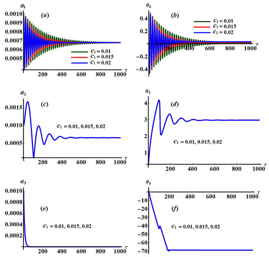
Figure 2. Relations of amplitudes $a_j(\tau )\hspace{0.17em}\hspace{0.17em}(j=1,2,3)$ and the modified phases ${\theta }_j(\tau )$ at $c_2=0.02,\hspace{0.17em}\hspace{0.17em}{c}_3=0.2$, ${\omega }_1=3.354,$ and ${\omega }_2=3.131$: (a–f) when $c_1(=0.01,0.015,0.02)$.

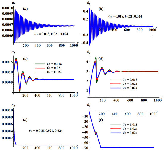
Figure 3. Relations of $a_j(\tau )\hspace{0.17em}\hspace{0.17em}(j=1,2,3)$ and ${\theta }_j(\tau )$ at $c_1=0.01,\hspace{0.17em}\hspace{0.17em}{c}_3=0.2,$ ${\omega }_1=3.354$ and ${\omega }_2=3.131$: (a–f) when $c_2(=0.018,0.021,0.024)$.

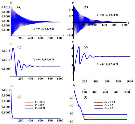
Figure 4. Characterization of the time histories of $a_j(\tau )\hspace{0.17em}\hspace{0.17em}(j=1,2,3)$ and ${\theta }_j(\tau )$ at $c_1=0.01,\hspace{0.17em}\hspace{0.17em}{c}_2=0.02,$ ${\omega }_1=3.354,$ and ${\omega }_2=3.131$: (a–f) when $c_3(=0.19,0.2,0.21)$.

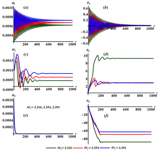
Figure 5. Changes of $a_j\hspace{0.17em}(j=1,2,3)$ and ${\theta }_j$ with $\tau$ at ${\omega }_2=3.131,$ $c_1=0.01,\hspace{0.17em}\hspace{0.17em}{c}_2=0.02,$ and $c_3=0.2$: (a–f) when ${\omega }_1(=3.316,3.354,3.391)$.

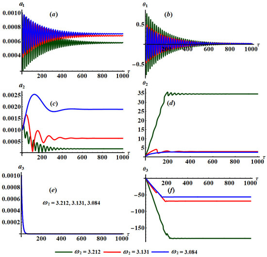
Figure 6. Changes of $a_j\hspace{0.17em}(j=1,2,3)$ and ${\theta }_j$ with $\tau$ at ${\omega }_1=3.354,$ $c_1=0.01,\hspace{0.17em}\hspace{0.17em}{c}_2=0.02,$ and $c_3=0.2$: (a–f) when ${\omega }_2(=3.212,3.131,3.084)$.

When the amplitudes $a_j$ and the adjusted phases ${\theta }_j$ are varied with time $\tau$ for distinct values of the damping coefficients $c_j\hspace{0.17em}\hspace{0.17em}(j=1,2,3)$ and the frequencies ${\omega }_k\hspace{0.17em}\hspace{0.17em}(k=1,2)$, we can predict that the above system (25) has a good influence according to these values.

A more in-depth study of Figure 2, Figure 3 and Figure 4 shows that they are calculated when $c_1(=0.01,0.015,0.02)$, $c_2(=0.018,0.021,0.024)$, and $c_3(=0.19,0.2,0.21)$, respectively. These figures are drawn at ${\omega }_1=3.354$ and ${\omega }_2=3.131$ when $(c_2=0.02,\hspace{0.17em}\hspace{0.17em}{c}_3=0.2),$ $(c_1=0.01,\hspace{0.17em}\hspace{0.17em}{c}_3=0.2),$ and $(c_1=0.01,\hspace{0.17em}\hspace{0.17em}{c}_2=0.02)$. Moreover, Figure 5 and Figure 6 are drawn at $c_1=0.01,$ $c_2=0.02,$ and $c_3=0.2$ when ${\omega }_1(=3.316,3.354,3.391)$ and ${\omega }_2(=3.212,3.131,3.084)$, respectively, for stationary values of ${\omega }_2=3.131$ as in Figure 5 and ${\omega }_1=3.354$ as in Figure 6.

According to the plotted curves in Figure 2, we observe that when $c_1$ has various values, the time histories of the amplitude $a_1$ and the adjusted phase ${\theta }_1$ behave as decaying waves until reaching a stationary behavior at the end of the investigated period of time, as seen in Figure 2a,b. The fluctuations of $a_2$ and ${\theta }_2$ waves with time $\tau$ become clear in the first quarter of the period of time and become stationary after that as explored in Figure 2c,d. On the other hand, a sharp descent of the curves describing the waves of $a_3$ and ${\theta }_3$ is observed in the curves of Figure 2e,f, which is due to the last two equations of the system (25). There is no variation of the $a_2,a_3$ and ${\theta }_2,{\theta }_3$ curves with the change of $c_1$ values due to the formulations of the equations of these curves.

The change of the various values of $c_2$ is evident in the curves describing the time histories of the amplitude $a_2$ and the modified phase ${\theta }_2$ because the third and fourth equations of system (25) are dependent on $c_2$, as seen in Figure 3c,d, while the other equations do not depend explicitly on $c_2$. Therefore, there is no variation, to some extent, of the curves describing $a_1,a_3$ and ${\theta }_1,{\theta }_3$ as drawn in the other parts of Figure 3.

Since the last two equations of system (25) depend on $c_3$, an observed variation of the curves describes the modified phase ${\theta }_3$, as seen in Figure 4f. There is no observed variation in the curves of the other variables because the first four equations of system (25) do not depend on $c_3$ explicitly as indicated in the other parts of Figure 4.

An examination of the system of equations (25) shows that these equations are dependent on ${\omega }_1$ and ${\omega }_2$. Therefore, we expect a good impact of these parameters on the time histories of $a_j\hspace{0.17em}\hspace{0.17em}(j=1,2,3)$ and ${\theta }_j$ which met with the plotted curves of Figure 5 and Figure 6. These curves describing the waves of these variables oscillate in a decaying manner as drawn in parts (a)–(d) of these figures or monotonically decrease with time as seen in parts (e) and (f) of the same figures. Based on this analysis, we come to the conclusion that the behavior of the system of equations (25) is stable and free of chaos.

Figure 7, Figure 8, Figure 9, Figure 10 and Figure 11 present the phase plane diagrams of $a_j\hspace{0.17em}(j=1,2,3)$ and ${\theta }_j$ when $c_j$ and ${\omega }_k\hspace{0.17em}\hspace{0.17em}(k=1,2)$ have various values. An inspection of the curves of these figures shows that we have spirals curves that are directed to one point, which gives an impression of the steady motion of these amplitudes and phases.

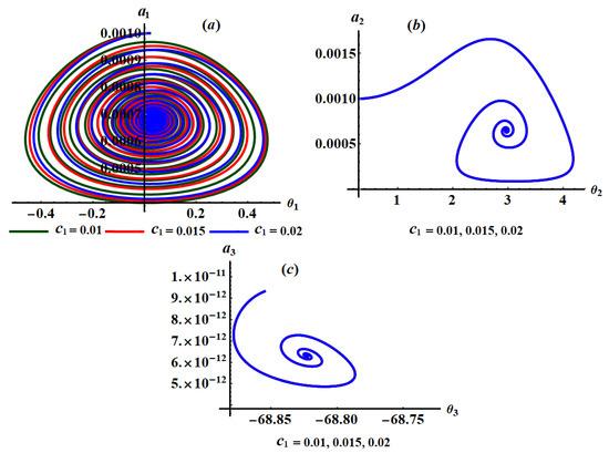
Figure 7. Phase planes $a_j{\theta }_j\hspace{0.17em}\hspace{0.17em}(j=1,2,3)$ at $c_2=0.02,\hspace{0.17em}\hspace{0.17em}{c}_3=0.2,\hspace{0.17em}\hspace{0.17em}{\omega }_1=3.354,$ and ${\omega }_2=3.131$: (a–c) when $c_1(=0.01,0.015,0.02)$.

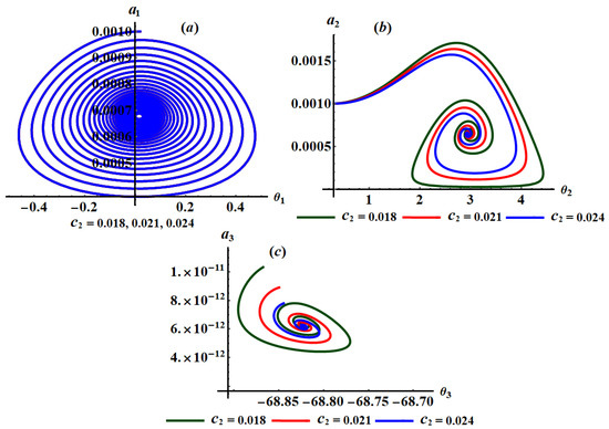
Figure 8. Phase planes $a_j{\theta }_j\hspace{0.17em}\hspace{0.17em}(j=1,2,3)$ at $c_1=0.01,\hspace{0.17em}\hspace{0.17em}{c}_3=0.2,$ ${\omega }_1=3.354$ and ${\omega }_2=3.131$: (a–c) when $c_2(=0.018,0.021,0.024)$.

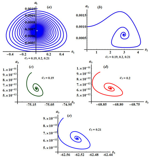
Figure 9. Phase planes $a_j{\theta }_j\hspace{0.17em}\hspace{0.17em}(j=1,2,3)$ when $c_1=0.01,\hspace{0.17em}\hspace{0.17em}{c}_2=0.02,\hspace{0.17em}\hspace{0.17em}{\omega }_1=3.354$ and ${\omega }_2=3.131$: (a,b) when $c_3(=0.19,0.2,0.21),$ (c) when $c_3=0.19,$ (d) when $c_3=0.2,$ and (e) when $c_3=0.21$.

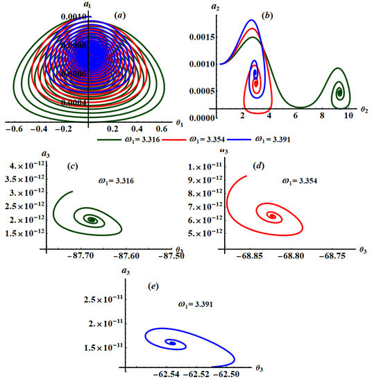
Figure 10. Phase planes $a_j{\theta }_j\hspace{0.17em}\hspace{0.17em}(j=1,2,3)$ at ${\omega }_2=3.131,$$c_1=0.01,\hspace{0.17em}\hspace{0.17em}{c}_2=0.02,$ and $c_3=0.2$: (a,b) when ${\omega }_1(=3.316,3.354,3.391),$ (c) when ${\omega }_1=3.316,$ (d) when ${\omega }_1=3.354,$ and (e) when ${\omega }_1=3.354$.

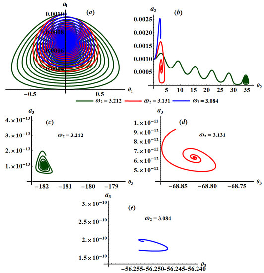
Figure 11. Phase planes $a_j{\theta }_j\hspace{0.17em}\hspace{0.17em}(j=1,2,3)$ at ${\omega }_1=3.354,$ $c_1=0.01,\hspace{0.17em}\hspace{0.17em}{c}_2=0.02,$ and $c_3=0.2$: (a,b) when ${\omega }_2(=3.212,3.131,3.084),$ (c) when ${\omega }_2=3.212,$ (d) when ${\omega }_2=3.131,$ and (e) when ${\omega }_2=3.084$.

Parts of Figure 7, Figure 8 and Figure 9 are drawn when $c_1,c_2,$ and $c_3$ have different values, respectively, to reveal the variation of curves of the phase planes $a_j{\theta }_j\hspace{0.17em}\hspace{0.17em}\hspace{0.17em}(j=1,2,3)$ with these values, while Figure 10 and Figure 11 describe the change of these planes that happened at different values of ${\omega }_1$ and ${\omega }_2$, respectively.

According to the curves of these figures and the system of equations (25), we observe that the plane $a_1{\theta }_1$ is impacted by the various values of $c_1$, as seen in Figure 7a, while there is no variation of the curves of planes $a_2{\theta }_2$ and $a_3{\theta }_3$ as indicated in Figure 7b,c. The curves of the phase planes $a_2{\theta }_2$ and $a_3{\theta }_3$ have been impacted with the variation of $c_2$ values of as seen in Figure 8b,c. On the other hand, there is no observed variation of the curves drawn in plane $a_1{\theta }_1$ when $c_2$ changes, as noticed in Figure 8a. According to the plotted curves in Figure 9, we can see that the curves shown in parts (a) and (b) that describe the phase planes $a_1{\theta }_1$ and $a_2{\theta }_2$ respectively, have no variation with various values of $c_3$. The good impact of the values of $c_3$ is observed in parts (c), (d), and (e) of Figure 9 for the phase plane $a_3{\theta }_3$.

The influence of the frequencies ${\omega }_1(=3.316,3.354,3.391)$ and ${\omega }_2(=3.212,3.131,3.084)$ on the phase plane diagrams $a_j{\theta }_j\hspace{0.17em}\hspace{0.17em}\hspace{0.17em}(j=1,2,3)$ is observed from the curves of Figure 10 and Figure 11, respectively. Therefore, we can say that these curves have a spiral form from the outside to the inside, and it is directed toward a single point for each curve, which means that all values of ${\omega }_k\hspace{0.17em}(k=1,2)$ have a significant impact on the curves of these planes. The reason goes back to the equations of system (25) that depend explicitly on ${\omega }_k\hspace{0.17em}(k=1,2)$.

It is important to remember that the obtained approximate solutions $z,\mathrm{\Phi },$ and $\eta$ describe the spring’s elongation, the rotation angle at the point $O_1$, and the elongation of the transverse absorber, respectively.

Figure 12, Figure 13, Figure 14, Figure 15 and Figure 16 depict the graphical representations of these solutions over time $\tau$, revealing their behaviors across the analyzed time interval as presented in parts (a), (b), and (c) when $\tau \in [0,100]$ and in parts (d), (e), and (f) when $\tau \in [0,1000]$ of these figures. Figure 12, Figure 13 and Figure 14 are performed at ${\omega }_1=3.354$ and ${\omega }_2=3.131$ at different values of $c_1(=0.01,0.015,0.02),$ $c_2(=0.018,0.021,0.024),$ and $c_3(=0.19,0.2,0.21)$ respectively. When these figures are compared with each other, we can see that the variations with different values of $c_j\hspace{0.17em}\hspace{0.17em}(j=1,2,3)$ seem to be slight. This is because the approximate solutions of the variables $z,\mathrm{\Phi },$ and $\eta$ do not depend on $c_j$ explicitly. In addition, Figure 15 and Figure 16 are portrayed at $c_1=0.01,$ $c_2=0.02,$ and $c_3=0.2$ when ${\omega }_1(=3.316,3.354,3.391)$ and ${\omega }_2(=3.212,3.131,3.084)$, respectively. It is noted that parts of Figure 15 have a phase shift, while parts of Figure 16 do not have a phase shift. The reason is that the curves of Figure 15 and Figure 16 are graphed when ${\omega }_1$ and ${\omega }_2$ have different values, respectively.

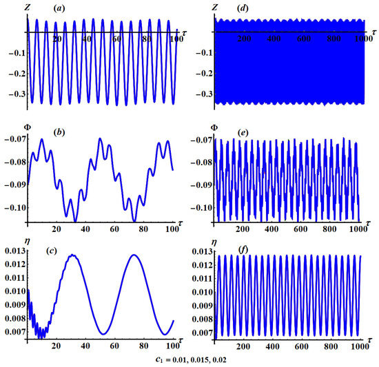
Figure 12. Solutions’ time histories when $c_1(=0.01,0.015,0.02),$ $c_2=0.02,$ $c_3=0.2,$ ${\omega }_1=3.354,$ and ${\omega }_2=3.131$: (a–c) at $\tau \in [0,100]$ and (d–f) at $\tau \in [0,1000]$.

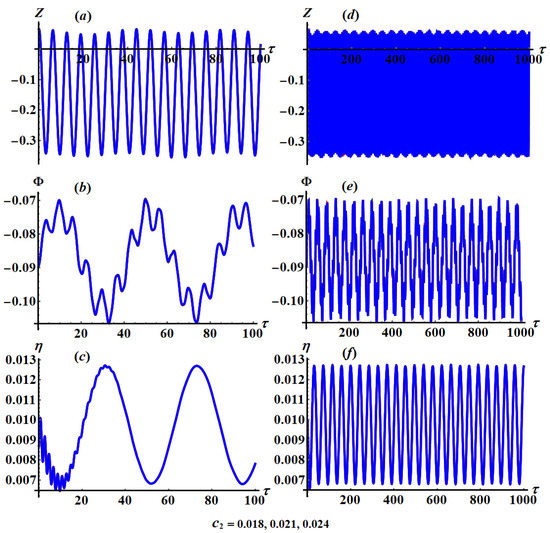
Figure 13. Change of $z,\mathrm{\Phi },$ and $\eta$ via $\tau$ when $c_1=0.01,\hspace{0.17em}\hspace{0.17em}{c}_2(=0.018,0.021,0.024),\hspace{0.17em}\hspace{0.17em}{c}_3=0.2,$ ${\omega }_1=3.354$ and ${\omega }_2=3.131$: (a–c) at $\tau \in [0,100]$ and (d–f) at $\tau \in [0,1000]$.

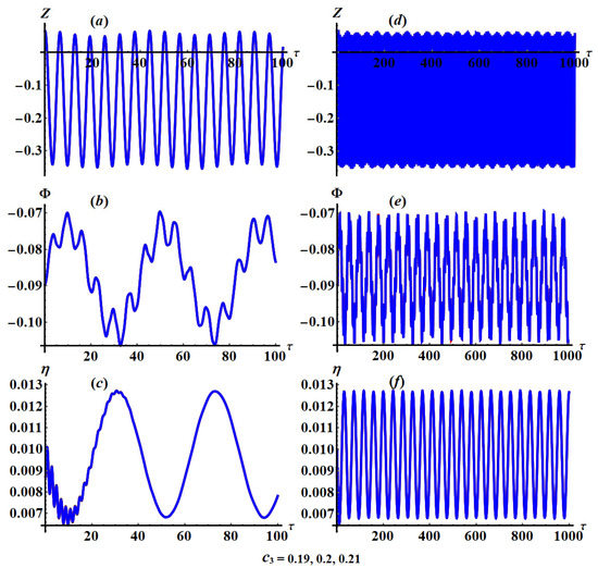
Figure 14. Evolution of solutions $z,\mathrm{\Phi },$ and $\eta$ throughout time $\tau$ at $c_3(=0.19,0.2,0.21),$ $c_1=0.01,$$c_2=0.02,$ ${\omega }_1=3.354,$ and ${\omega }_2=3.131$: (a–c) at $\tau \in [0,100]$ and (d–f) at $\tau \in [0,1000]$.

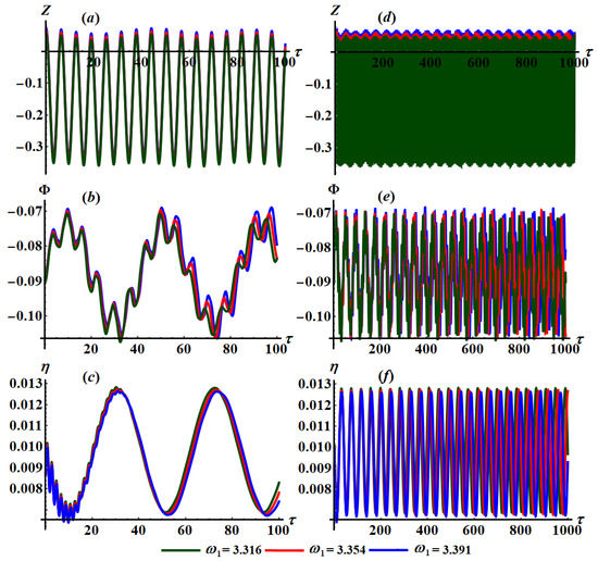
Figure 15. Progression of solutions $z,\mathrm{\Phi },$ and $\eta$ over time $\tau$ when ${\omega }_1(=3.316,3.354,3.391),$ ${\omega }_2=3.131,$ $c_1=0.01,$ $c_2=0.02,$ and $c_3=0.2$: (a–c) at $\tau \in [0,100]$ and (d–f) at $\tau \in [0,1000]$.

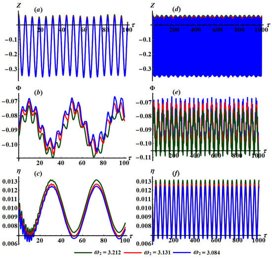
Figure 16. Solutions’ temporal histories when ${\omega }_2(=3.212,3.131,3.084),$ ${\omega }_1=3.354,$ $c_1=0.01,$ $c_2=0.02,$ and $c_3=0.2$: (a–c) at $\tau \in [0,100]$ and (d–f) at $\tau \in [0,1000]$.

Based on the sketched curves of the solutions $z,\mathrm{\Phi },$ and $\eta$, we observe that the waves describing these solutions have a periodic manner in which the number of oscillations and their wavelengths remain stationary to some extent with the variation of $c_j\hspace{0.17em}(j=1,2,3)$ values. Parts (a) of these figures have an explicitly periodic form for the wave of the solution $z$. It is notable from parts (b) of these figures that each period of the wave contains a constant number of vibrations that are repeated for each period. This is due to the analytical form of the rotation angle $\mathrm{\Phi }$, in which its behavior has a spinning form. On the other hand, the wave describing spring’s elongation $\eta$ experiences rapid oscillations at the beginning of the motion due to the absorber’s effect and damping impact on the investigated dynamical system, in which it settles down after that and vanishes at the end of time interval, as seen in parts (c) of these figures.

According to the calculations of Figure 15 and Figure 16, we get to the conclusion that the change of the ${\omega }_k\hspace{0.17em}(k=1,2)$ values has a considerable impact on the attitude of the describing waves of the attained solutions. Regardless of the fact that the wave’s behavior of the solutions is periodic, we observe that the amplitudes of these waves increase and decrease with the increasing of ${\omega }_k$ as seen in Figure 15a–f and Figure 16a–f, respectively.

5. Steady state Solutions

The major objective of the present section is to study the oscillations of the examined system in the case of steady state. From the equations of system (25), we can obtain both of the modified phases ${\theta }_j\hspace{0.17em}\hspace{0.17em}(j=1,2,3)$ and amplitudes $a_j$ in the steady state case. Alternatively, the zero values of the left-hand sides of the equations of this system are considered. Therefore, we consider $\frac{d{a}_j}{d\tau }=0$ and $\hspace{0.17em}\hspace{0.17em}\frac{d{\theta }_j}{d\tau }=0$ [32], to obtain the next algebraic system of six equations of the functions ${\theta }_j$ and $a_j$.

$$\begin{gathered} \begin{array}{cc}{f}_1\sin {\theta }_1\hfill & -c_1{a}_1=0,\hfill \\ f_1\cos {\theta }_1\hfill & +2a_1[{\sigma }_1-\alpha z_r-\frac{{(1+w_1^2)}^2}{2(1-w_1^2)}{r}^2{\beta }^2-\frac{3(1-w_1^2)}{4(1-4\hspace{0.17em}{w}_1^2)}{w}_1^2{a}_2^2]=0,\hfill \\ m_0\sin {\theta }_2\hfill & -w_1{c}_2{a}_2=0,\hfill \\ m_0\cos {\theta }_2\hfill & +2\hspace{0.17em}{w}_1{a}_2\{{\sigma }_2-w_1(\alpha z_r^2-r^2\beta +\frac{(1-w_1^2)}{8(1-4\hspace{0.17em}{w}_1^2)}[12a_1^2-(1+8\hspace{0.17em}{w}_1^2)a_2^2]\hfill \\ & -\frac{r^2{\beta }^2}{4(1-w_1^2)\hspace{0.17em}{w}_2^2}[(14-3r^2)\hspace{0.17em}{w}_2^2-2(4-w_2^2)\hspace{0.17em}{w}_1^4+(8+3r^2{w}_2^2)\hspace{0.17em}{w}_1^2])\}=0,\hfill \end{array} \\ \begin{array}{cc}\frac{(1-w_1^2)}{(1-4\hspace{0.17em}{w}_1^2)}{w}_1^2{a}_2^3\sin {\theta }_3+w_2{c}_3{a}_3=0,\hfill & \\ \frac{(1-w_1^2)}{(1-4\hspace{0.17em}{w}_1^2)}{w}_1^2{a}_2^3\cos {\theta }_3-2\hspace{0.17em}{w}_2{a}_3\{{\sigma }_3+3\hspace{0.17em}{w}_1\{\alpha z_r^2-r^2\beta +\frac{(1-w_1^2)}{8(1-4\hspace{0.17em}{w}_1^2)}[12a_1^2\hfill & \\ -(1+8\hspace{0.17em}{w}_1^2)a_2^2]-\frac{r^2{\beta }^2}{4(1-w_1^2)\hspace{0.17em}{w}_2^2}[(14-3r^2)\hspace{0.17em}{w}_2^2-2(4-w_2^2)\hspace{0.17em}{w}_1^4+(8+3r^2{w}_2^2)\hspace{0.17em}{w}_1^2]\}\hfill & \\ -\frac{3m_0}{2\hspace{0.17em}{w}_1{a}_2}\cos {\theta }_2+\frac{1}{2\hspace{0.17em}{w}_2}[\beta (w_1^2-w_2^2)+\frac{1}{2}{w}_1^2{a}_2^2+\frac{{\beta }^2}{4\hspace{0.17em}{w}_2^2}(4r^2{w}_2^4+4\hspace{0.17em}{w}_2^2(w_1^2-w_2^2)\hfill & \\ +{(w_1^2-w_2^2)}^2)]\}=0,\hfill & \end{array} \end{gathered}$$

(26)

Now, we can remove the adjusted phases ${\theta }_j$ from the preceding system to produce the following three non-linear algebraic equations between longitudinal amplitude $a_1$, the swing oscillations $a_2$, and the frequency represented by the detuning parameters ${\sigma }_j$ and the absorber’s amplitude $a_3$.

$$\begin{array}{cc}{f}_1^2& =a_1^2\{c_1^2+4{[{\sigma }_1-\alpha z_r-\frac{{(1+w_1^2)}^2}{2(1-w_1^2)}{r}^2{\beta }^2-\frac{3(1-w_1^2)}{4(1-4\hspace{0.17em}{w}_1^2)}{w}_1^2{a}_2^2]}^2\},\hfill \\ m_0^2& =w_1^2{a}_2^2\{c_2^2+4[{\sigma }_2-w_1(\alpha z_r^2-r^2\beta +\frac{(1-w_1^2)}{8(1-4\hspace{0.17em}{w}_1^2)}[12a_1^2-(1+8\hspace{0.17em}{w}_1^2)a_2^2]\hfill \\ & -\frac{r^2{\beta }^2}{4(1-w_1^2)w_2^2}[(14-3r^2)\hspace{0.17em}{w}_2^2-2(4-w_2^2)\hspace{0.17em}{w}_1^4+(8+3r^2{w}_2^2)\hspace{0.17em}{w}_1^2]){]}^2\},\hfill \\ \frac{{(1-w_1^2)}^2}{{(1-4\hspace{0.17em}{w}_1^2)}^2}{w}_1^4& =w_2^2{a}_3^2\{c_3^2+4[{\sigma }_3+3{\sigma }_2+\frac{1}{8\hspace{0.17em}{w}_2^3}({\beta }^2{w}_1^4+2(2\beta +{\beta }^2+a_2^2)w_1^2{w}_2^2\hfill \\ & -\beta [4+(3-4r^2)\beta ]w_2^4){]}^2\}.\hfill \end{array}$$

(27)

Stability testing is considered a crucial aspect of the vibrations in the steady state case. To explore such a circumstance, the behavior of the system in a domain relatively near to fixed points is investigated. Therefore, the substitutions listed below are employed in (25) to achieve this purpose.

$$\begin{array}{l}{a}_1=a_{10}+a_{11},\hspace{0.17em}\hspace{0.17em}\hspace{0.17em}\hspace{0.17em}\hspace{0.17em}\hspace{0.17em}\hspace{0.17em}\hspace{0.17em}\hspace{0.17em}\hspace{0.17em}\hspace{0.17em}\hspace{0.17em}\hspace{0.17em}\hspace{0.17em}\hspace{0.17em}{\theta }_1={\theta }_{10}+{\theta }_{11},\\ a_2=a_{20}+a_{21},\hspace{0.17em}\hspace{0.17em}\hspace{0.17em}\hspace{0.17em}\hspace{0.17em}\hspace{0.17em}\hspace{0.17em}\hspace{0.17em}\hspace{0.17em}\hspace{0.17em}\hspace{0.17em}\hspace{0.17em}\hspace{0.17em}\hspace{0.17em}{\theta }_2={\theta }_{20}+{\theta }_{21},\\ a_3=a_{30}+a_{31},\hspace{0.17em}\hspace{0.17em}\hspace{0.17em}\hspace{0.17em}\hspace{0.17em}\hspace{0.17em}\hspace{0.17em}\hspace{0.17em}\hspace{0.17em}\hspace{0.17em}\hspace{0.17em}\hspace{0.17em}\hspace{0.17em}\hspace{0.17em}{\theta }_3={\theta }_{30}+{\theta }_{31}.\end{array}$$

(28)

Here, $a_{j0}$ and ${\theta }_{j0}\hspace{0.17em}\hspace{0.17em}(j=1,2,3)$ denote the steady state solutions, whereas $a_{j1}$ and ${\theta }_{j1}$ represent relatively small disturbances in relation to $a_{j0}$ and ${\theta }_{j0}$. As a result of linearization and the reality of the fixed points of (25), we get

$$\begin{array}{cc}\frac{d{a}_{11}}{d\tau }& =\frac{1}{2}(f_1{\theta }_{11}\cos {\theta }_{10}-c_1{a}_{11}),\hfill \\ a_{10}\frac{d{\theta }_{11}}{d\tau }& =a_{11}[{\sigma }_1-\alpha z_r-\frac{{(1+w_1^2)}^2}{2(1-w_1^2)}{r}^2{\beta }^2]-\frac{3(1-w_1^2)}{4(1-4\hspace{0.17em}{w}_1^2)}{w}_1^2{a}_{20}(a_{20}{a}_{11}+2a_{10}{a}_{21})\hfill \\ & +\frac{1}{2}{f}_1{\theta }_{11}\sin {\theta }_{10},\hfill \\ \frac{d{a}_{21}}{d\tau }& =\frac{1}{2}(\frac{m_0}{w_1}{\theta }_{21}\cos {\theta }_{20}-c_2{a}_{21}),\hfill \\ a_{20}\frac{d{\theta }_{21}}{d\tau }& =a_{21}\{{\sigma }_2-w_1(\alpha z_r^2-r^2\beta -\frac{r^2{\beta }^2}{4(1-w_1^2)\hspace{0.17em}{w}_2^2}[(14-3r^2)\hspace{0.17em}{w}_2^2-2(4-w_2^2)\hspace{0.17em}{w}_1^4)\hfill \\ & +(8+3r^2{w}_2^2)\hspace{0.17em}{w}_1^2])\}-\frac{(1-w_1^2)w_1}{8(1-4\hspace{0.17em}{w}_1^2)}[12a_{10}(a_{10}{a}_{21}+2a_{20}{a}_{11})\hfill \\ & -3(1+8\hspace{0.17em}{w}_1^2)a_{20}^2{a}_{21}]-\frac{m_0}{2\hspace{0.17em}{w}_1}{\theta }_{21}\sin {\theta }_{20},\hfill \\ \frac{d{a}_{31}}{d\tau }& =-\frac{1}{2}[\frac{(1-w_1^2)w_1^2}{(1-4\hspace{0.17em}{w}_1^2)w_2}{a}_{20}^2(a_{20}{\theta }_{31}\cos {\theta }_{30}+3a_{21}\sin {\theta }_{30})+c_3{a}_{31}],\hfill \\ a_{20}{a}_{30}\frac{d{\theta }_{31}}{d\tau }& =(a_{20}{a}_{31}+a_{21}{a}_{30})\{{\sigma }_3+3\hspace{0.17em}{w}_1(\alpha z_r^2-r^2\beta -\frac{r^2{\beta }^2}{4(1-w_1^2)w_2^2}[(14-3r^2)\hspace{0.17em}{w}_2^2\hfill \\ & -2(4-w_2^2)\hspace{0.17em}{w}_1^4+(8+3r^2{w}_2^2)\hspace{0.17em}{w}_1^2])+\frac{1}{2\hspace{0.17em}{w}_2}[\beta (w_1^2-w_2^2)+\frac{{\beta }^2}{4\hspace{0.17em}{w}_2^2}(4r^2{w}_2^4\hfill \\ & +4\hspace{0.17em}{w}_2^2(w_1^2-w_2^2)+{(w_1^2-w_2^2)}^2)]\}+\frac{3(1-w_1^2)}{8(1-4\hspace{0.17em}{w}_1^2)}{w}_1[12a_{10}(a_{10}{a}_{20}{a}_{31}\hfill \\ & +a_{10}{a}_{30}{a}_{21}+2a_{20}{a}_{30}{a}_{11})-(1+8\hspace{0.17em}{w}_1^2)(a_{20}^3{a}_{31}+3a_{20}^2{a}_{30}{a}_{21})]+\frac{w_1^2}{4\hspace{0.17em}{w}_2}\hfill \\ & \times (a_{20}^3{a}_{31}+3a_{20}^2{a}_{30}{a}_{21})\hspace{0.17em}-\frac{3m_0}{2\hspace{0.17em}{w}_1}(a_{31}\cos {\theta }_{20}-a_{30}{\theta }_{21}\sin {\theta }_{20})\hfill \\ & -\frac{(1-w_1^2)\hspace{0.17em}{w}_1^2}{2(1-4\hspace{0.17em}{w}_1^2)\hspace{0.17em}{w}_2}{a}_{20}^3(4a_{21}\cos {\theta }_{30}-a_{20}{\theta }_{31}\sin {\theta }_{30}).\hfill \end{array}$$

(29)

Since $a_{j1}$ and ${\theta }_{j1}\hspace{0.17em}\hspace{0.17em}(j=1,2,3)$ are perturbed functions of amplitudes and phases of the aforementioned linear system. Then, the linear function $k_s{e}^{\lambda \tau }\hspace{0.17em}\hspace{0.17em}(s=1,2,3,4,5,6)$ of the exponential form can be used to express about their solutions, where $k_s$ and $\lambda$ are constants and the perturbation’s eigenvalue, respectively. The real parts of the roots of the next characteristic equation of (29) should be negative if the steady state solutions are asymptotically stable [33,34].

$${\lambda }^6+{\Gamma }_1{\lambda }^5+{\Gamma }_2{\lambda }^4+{\Gamma }_3{\lambda }^3+{\Gamma }_4{\lambda }^2+{\Gamma }_5\lambda +{\Gamma }_6=0,$$

(30)

where ${\Gamma }_s\hspace{0.17em}\hspace{0.17em}(s=1,2,\dots ,6)$ are functions of $a_{j0},{\theta }_{j0},$ and $c_j$ (see Appendix B).

The required and sufficient requirements of stability for certain solutions at steady state can be expressed as follows

$$\begin{array}{c}{\Gamma }_1>0,\hspace{0.17em}\hspace{0.17em}\hspace{0.17em}\hspace{0.17em}\hspace{0.17em}\hspace{0.17em}\hspace{0.17em}\hspace{0.17em}\hspace{0.17em}\hspace{0.17em}\hspace{0.17em}\hspace{0.17em}\hspace{0.17em}\hspace{0.17em}\hspace{0.17em}\hspace{0.17em}\hspace{0.17em}\hspace{0.17em}\hspace{0.17em}{\Gamma }_3({\Gamma }_1{\Gamma }_2-{\Gamma }_3)-{\Gamma }_4{\Gamma }_1^2+{\Gamma }_1{\Gamma }_5>0,\hspace{0.17em}\hspace{0.17em}\hspace{0.17em}\hspace{0.17em}\hspace{0.17em}\hspace{0.17em}\hspace{0.17em}\hspace{0.17em}\hspace{0.17em}\hspace{0.17em}\hspace{0.17em}\hspace{0.17em}\hspace{0.17em}\hspace{0.17em}\hspace{0.17em}\hspace{0.17em}\hspace{0.17em}\hspace{0.17em}\hspace{0.17em}\hspace{0.17em}{\Gamma }_1{\Gamma }_2-{\Gamma }_3>0,\hfill \\ & \\ {\Gamma }_3{\Gamma }_4({\Gamma }_1{\Gamma }_2-{\Gamma }_3)-{\Gamma }_1^2{\Gamma }_4^2-{\Gamma }_1{\Gamma }_2^2{\Gamma }_5+{\Gamma }_2{\Gamma }_3{\Gamma }_5+2{\Gamma }_1{\Gamma }_4{\Gamma }_5-{\Gamma }_5^2+{\Gamma }_1^2{\Gamma }_2{\Gamma }_6-{\Gamma }_1{\Gamma }_3{\Gamma }_6>0,\hfill \\ & \\ {\Gamma }_1{\Gamma }_2{\Gamma }_3{\Gamma }_4{\Gamma }_5-{\Gamma }_3^2{\Gamma }_4{\Gamma }_5-{\Gamma }_1^2{\Gamma }_4^2{\Gamma }_5-{\Gamma }_1{\Gamma }_2^2{\Gamma }_5^2+{\Gamma }_2{\Gamma }_3{\Gamma }_5^2+2{\Gamma }_1{\Gamma }_4{\Gamma }_5^2-{\Gamma }_5^3-{\Gamma }_1{\Gamma }_2{\Gamma }_3^2{\Gamma }_6\hfill \\ +{\Gamma }_3^3{\Gamma }_6+{\Gamma }_1^2{\Gamma }_3{\Gamma }_4{\Gamma }_6+2{\Gamma }_1^2{\Gamma }_2{\Gamma }_5{\Gamma }_6-3{\Gamma }_1{\Gamma }_3{\Gamma }_5{\Gamma }_6-{\Gamma }_1^3{\Gamma }_6^2>0,\hfill \\ & \\ {\Gamma }_6({\Gamma }_1{\Gamma }_2{\Gamma }_3{\Gamma }_4{\Gamma }_5-{\Gamma }_3^2{\Gamma }_4{\Gamma }_5-{\Gamma }_1^2{\Gamma }_4^2{\Gamma }_5-{\Gamma }_1{\Gamma }_2^2{\Gamma }_5^2+{\Gamma }_2{\Gamma }_3{\Gamma }_5^2+2{\Gamma }_1{\Gamma }_4{\Gamma }_5^2-{\Gamma }_5^3-{\Gamma }_1{\Gamma }_2{\Gamma }_3^2{\Gamma }_6\hfill \\ +{\Gamma }_3^3{\Gamma }_6+{\Gamma }_1^2{\Gamma }_3{\Gamma }_4{\Gamma }_6+2{\Gamma }_1^2{\Gamma }_2{\Gamma }_5{\Gamma }_6-3{\Gamma }_1{\Gamma }_3{\Gamma }_5{\Gamma }_6-{\Gamma }_1^3{\Gamma }_6^2)>0.\hfill \end{array}$$

(31)

6. The Stability Analysis

In this section, we investigate the model’s stability as well as its non-linear evolution using the Routh–Hurwitz non-linear stability approach. It must be remembered that a damped spring connected with a transverse absorber under the action of $F(t)$ and $M(t)$. Some factors have been revealed to play a substantial impact in the stability processes such as damping’s constants $c_j\hspace{0.17em}\hspace{0.17em}(j=1,2,3)$, frequencies ${\omega }_k\hspace{0.17em}(k=1,2)$, and parameters of detuning ${\sigma }_j$. To gain the stability plots of system (25), a specific process with various parameters of the system has been used. The adjusted amplitudes $a_j\hspace{0.17em}\hspace{0.17em}(j=1,2,3)$ plotted via time are for various parametrical regions, in addition to the graphical representations of their characteristics through the phase plane paths. Curves of frequency responses of $a_j$ versus ${\sigma }_2$ and the system’s fixed points have been portrayed in Figure 17, Figure 18, Figure 19, Figure 20, Figure 21, Figure 22, Figure 23, Figure 24, Figure 25, Figure 26, Figure 27, Figure 28, Figure 29, Figure 30 and Figure 31, in which the flowing data have been taken into account besides the previous ones.

$$\begin{array}{l}{\sigma }_1=(-0.001,0,0.001),\hspace{0.17em}\hspace{0.17em}\hspace{0.17em}\hspace{0.17em}{\sigma }_3=0.001,\hspace{0.17em}\hspace{0.17em}\hspace{0.17em}\hspace{0.17em}{p}_1=1+{\sigma }_1,\\ p_2=w_1+{\sigma }_2,\hspace{0.17em}\hspace{0.17em}\hspace{0.17em}\hspace{0.17em}3w_1=w_2+{\sigma }_3,\hspace{0.17em}\hspace{0.17em}\hspace{0.17em}\hspace{0.17em}{f}_1=0.0004,\hspace{0.17em}\hspace{0.17em}\hspace{0.17em}\hspace{0.17em}{m}_0=0.00007.\end{array}$$

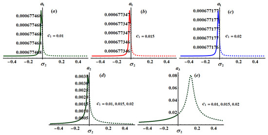
Figure 17. Frequency response for $a_j\hspace{0.17em}\hspace{0.17em}(j=1,2,3)$ via ${\sigma }_2$ at when $c_2=0.02,\hspace{0.17em}\hspace{0.17em}{c}_3=0.2,$${\omega }_1=3.354,$ ${\omega }_2=3.131,$ and ${\sigma }_1=-0.001$: (a) when $c_1=0.01,$ (b) when $c_1=0.015,$ (c) when $c_1=0.02,$ and (d,e) when $c_1(=0.01,\hspace{0.17em}0.015,\hspace{0.17em}0.02)$.

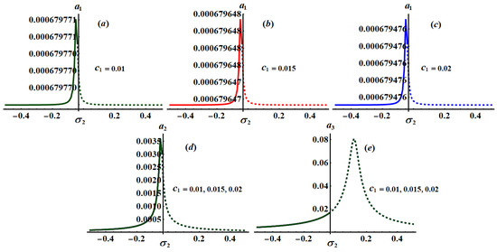
Figure 18. Frequency response of $a_j\hspace{0.17em}\hspace{0.17em}(j=1,2,3)$ via ${\sigma }_2$ at $c_2=0.02,\hspace{0.17em}\hspace{0.17em}{c}_3=0.2,\hspace{0.17em}\hspace{0.17em}{\omega }_1=3.354,\hspace{0.17em}\hspace{0.17em}{\omega }_2=3.131,$ and ${\sigma }_1=0:$(a) when $c_1=0.01,$ (b) when $c_1=0.015,$ (c) when $c_1=0.02,$ and (d,e) when $c_1(=0.01,\hspace{0.17em}0.015,\hspace{0.17em}0.02)$.

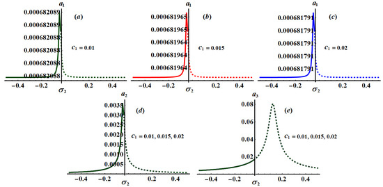
Figure 19. Frequency response of $a_j\hspace{0.17em}\hspace{0.17em}(j=1,2,3)$ via ${\sigma }_2$ at $c_2=0.02,\hspace{0.17em}\hspace{0.17em}{c}_3=0.2,\hspace{0.17em}\hspace{0.17em}{\omega }_1=3.354,$ ${\omega }_2=3.131,$ and ${\sigma }_1=0.001:$(a) when $c_1=0.01,$ (b) when $c_1=0.015,$ (c) when $c_1=0.02,$ and (d,e) when $c_1(=0.01,\hspace{0.17em}0.015,\hspace{0.17em}0.02)$.

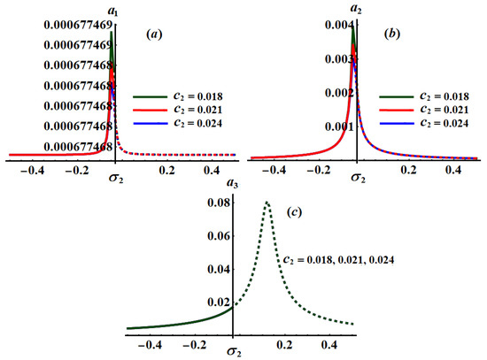
Figure 20. Curves of the planes ${\sigma }_2{a}_j\hspace{0.17em}\hspace{0.17em}(j=1,2,3)$ at when $c_1=0.01,\hspace{0.17em}\hspace{0.17em}{c}_3=0.2,\hspace{0.17em}\hspace{0.17em}{\omega }_1=3.354,\hspace{0.17em}\hspace{0.17em}{\omega }_2=3.131,$ and ${\sigma }_1=-0.001$: (a–c) when $c_2(=0.018,\hspace{0.17em}0.021,\hspace{0.17em}0.024)$.

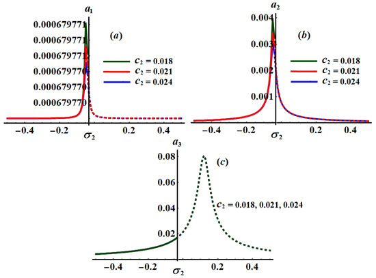
Figure 21. Curves of the planes ${\sigma }_2{a}_j\hspace{0.17em}\hspace{0.17em}(j=1,2,3)$ at $c_1=0.01,\hspace{0.17em}\hspace{0.17em}{c}_3=0.2,\hspace{0.17em}\hspace{0.17em}{\omega }_1=3.354,\hspace{0.17em}\hspace{0.17em}{\omega }_2=3.131,$ and ${\sigma }_1=0$: (a–c) when $c_2(=0.018,\hspace{0.17em}0.021,\hspace{0.17em}0.024)$.

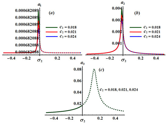
Figure 22. Curves of the planes ${\sigma }_2{a}_j\hspace{0.17em}\hspace{0.17em}(j=1,2,3)$ at $c_1=0.01,\hspace{0.17em}\hspace{0.17em}{c}_3=0.2,\hspace{0.17em}\hspace{0.17em}{\omega }_1=3.354,\hspace{0.17em}\hspace{0.17em}{\omega }_2=3.131,$ and ${\sigma }_1=0.001$: (a–c) when $c_2(=0.018,\hspace{0.17em}0.021,\hspace{0.17em}0.024)$.

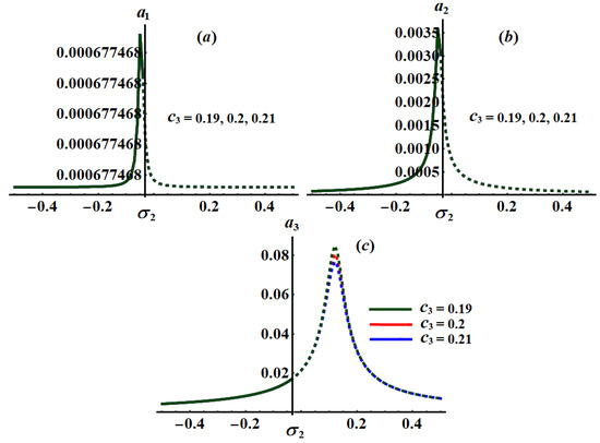
Figure 23. Curves of the planes ${\sigma }_2{a}_j\hspace{0.17em}\hspace{0.17em}(j=1,2,3)$ at $c_1=0.01,\hspace{0.17em}\hspace{0.17em}{c}_2=0.02,\hspace{0.17em}\hspace{0.17em}{\omega }_1=3.354,\hspace{0.17em}\hspace{0.17em}{\omega }_2=3.131,$ and ${\sigma }_1=-0.001$: (a–c) when $c_3(=0.19,\hspace{0.17em}0.2,\hspace{0.17em}0.21)$.

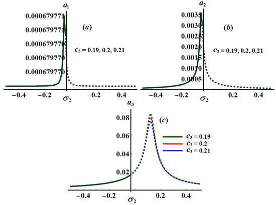
Figure 24. Curves of the planes ${\sigma }_2{a}_j\hspace{0.17em}\hspace{0.17em}(j=1,2,3)$ at $c_1=0.01,\hspace{0.17em}\hspace{0.17em}{c}_2=0.02,\hspace{0.17em}\hspace{0.17em}{\omega }_1=3.354,\hspace{0.17em}\hspace{0.17em}{\omega }_2=3.131,$ and ${\sigma }_1=0$: (a–c) when $c_3(=0.19,\hspace{0.17em}0.2,\hspace{0.17em}0.21)$.

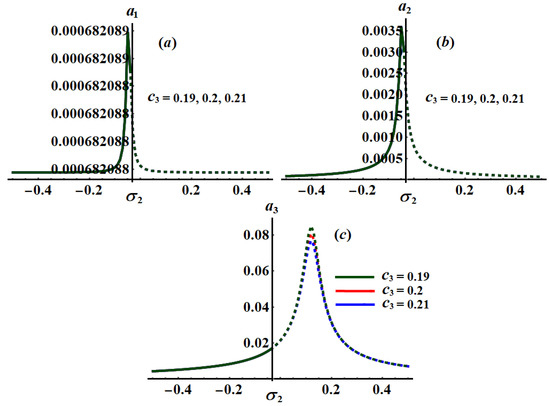
Figure 25. Curves of the planes ${\sigma }_2{a}_j\hspace{0.17em}\hspace{0.17em}(j=1,2,3)$ at $c_1=0.01,\hspace{0.17em}\hspace{0.17em}{c}_2=0.02,\hspace{0.17em}\hspace{0.17em}{\omega }_1=3.354,\hspace{0.17em}\hspace{0.17em}{\omega }_2=3.131,$ and ${\sigma }_1=0.001$: (a–c) when $c_3(=0.19,\hspace{0.17em}0.2,\hspace{0.17em}0.21)$.

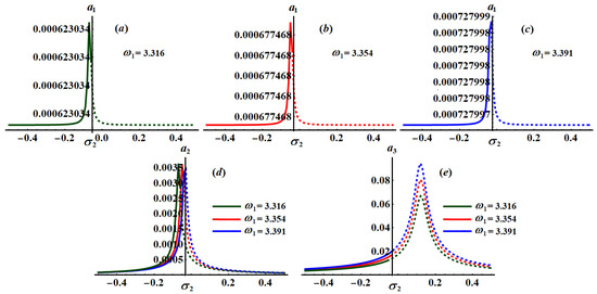
Figure 26. Curves of the planes ${\sigma }_2{a}_j\hspace{0.17em}\hspace{0.17em}(j=1,2,3)$ at ${\omega }_2=3.131,\hspace{0.17em}\hspace{0.17em}{c}_1=0.01,\hspace{0.17em}\hspace{0.17em}{c}_2=0.02,\hspace{0.17em}\hspace{0.17em}{c}_3=0.2,$ and ${\sigma }_1=-0.001$: (a) when ${\omega }_1=3.316,\hspace{0.17em}$ (b) when ${\omega }_1=\hspace{0.17em}3.354,\hspace{0.17em}$ (c) when ${\omega }_1=\hspace{0.17em}3.391,$ and (d,e) when ${\omega }_1(=3.316,\hspace{0.17em}3.354,\hspace{0.17em}3.391)$.

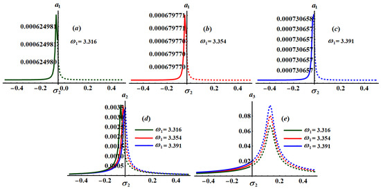
Figure 27. Curves of the planes ${\sigma }_2{a}_j\hspace{0.17em}\hspace{0.17em}(j=1,2,3)$ at ${\omega }_2=3.131,\hspace{0.17em}\hspace{0.17em}{c}_1=0.01,\hspace{0.17em}\hspace{0.17em}{c}_2=0.02,\hspace{0.17em}\hspace{0.17em}{c}_3=0.2,$ and ${\sigma }_1=0:$ (a) when ${\omega }_1=3.316,\hspace{0.17em}$ (b) when ${\omega }_1=\hspace{0.17em}3.354,\hspace{0.17em}$ (c) when ${\omega }_1=\hspace{0.17em}3.391,$ and (d,e) when ${\omega }_1(=3.316,\hspace{0.17em}3.354,\hspace{0.17em}3.391)$.

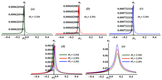
Figure 28. Curves of the planes ${\sigma }_2{a}_j\hspace{0.17em}\hspace{0.17em}(j=1,2,3)$ at ${\omega }_2=3.131,\hspace{0.17em}\hspace{0.17em}{c}_1=0.01,\hspace{0.17em}\hspace{0.17em}{c}_2=0.02,\hspace{0.17em}\hspace{0.17em}{c}_3=0.2,$ and ${\sigma }_1=0.001:$(a) when ${\omega }_1=3.316,\hspace{0.17em}$ (b) when ${\omega }_1=\hspace{0.17em}3.354,\hspace{0.17em}$ (c) when ${\omega }_1=\hspace{0.17em}3.391,$ and (d,e) when ${\omega }_1(=3.316,\hspace{0.17em}3.354,\hspace{0.17em}3.391)$.

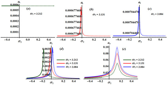
Figure 29. Curves of the planes ${\sigma }_2{a}_j\hspace{0.17em}\hspace{0.17em}(j=1,2,3)$ at when ${\omega }_1=3.354,\hspace{0.17em}\hspace{0.17em}{c}_1=0.01,\hspace{0.17em}\hspace{0.17em}{c}_2=0.02,\hspace{0.17em}\hspace{0.17em}{c}_3=0.2,$ and ${\sigma }_1=-0.001:$(a) when ${\omega }_2=3.212,$ (b) when ${\omega }_2=\hspace{0.17em}3.131,$ (c) when ${\omega }_2=\hspace{0.17em}3.084,$ and (d,e) when ${\omega }_2(=3.212,\hspace{0.17em}3.131,\hspace{0.17em}3.084)$.

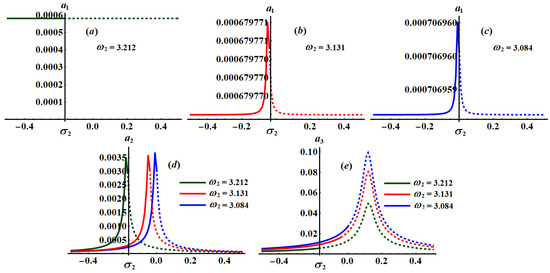
Figure 30. Curves of the planes ${\sigma }_2{a}_j\hspace{0.17em}\hspace{0.17em}(j=1,2,3)$ at ${\omega }_1=3.354,\hspace{0.17em}\hspace{0.17em}{c}_1=0.01,\hspace{0.17em}\hspace{0.17em}{c}_2=0.02,\hspace{0.17em}\hspace{0.17em}{c}_3=0.2,$ and ${\sigma }_1=0:$(a) when ${\omega }_2=3.212,$ (b) when ${\omega }_2=\hspace{0.17em}3.131,$ (c) when ${\omega }_2=\hspace{0.17em}3.084,$ and (d,e) when ${\omega }_2(=3.212,\hspace{0.17em}3.131,\hspace{0.17em}3.084)$.

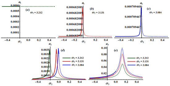
Figure 31. Curves of the planes ${\sigma }_2{a}_j\hspace{0.17em}\hspace{0.17em}(j=1,2,3)$ when ${\omega }_1=3.354,\hspace{0.17em}\hspace{0.17em}{c}_1=0.01,\hspace{0.17em}\hspace{0.17em}{c}_2=0.02,\hspace{0.17em}\hspace{0.17em}{c}_3=0.2,$ and ${\sigma }_1=-0.001:$ (a) at ${\omega }_2=3.212,$ (b) at ${\omega }_2=3.131,$ (c) at ${\omega }_2=3.084,$ and (d,e) at ${\omega }_2(=3.212,\hspace{0.17em}3.131,\hspace{0.17em}3.084)$.

The significance impact of the damping coefficient $c_1$ has been explored in the curves of Figure 17, Figure 18 and Figure 19 when ${\sigma }_1=-0.001,$ ${\sigma }_1=0,$ and ${\sigma }_1=0.001$, respectively. The impact of $c_2$ and $c_3$, for the same values of ${\sigma }_1$, has been indicated in Figure 20, Figure 21, Figure 22, Figure 23, Figure 24 and Figure 25. The inspection of parts of Figure 17, Figure 18 and Figure 19 shows the effect of the selected values of $c_1=(0.01,\hspace{0.17em}0.015,\hspace{0.17em}0.02)$ on the frequency response curves when $c_2=0.02,$ $c_3=0.2,$ ${\omega }_1=3.354$ and ${\omega }_2=3.131$.

It is obvious that $c_1$ has a bigger role on the curves of plane $a_1{\sigma }_2$ than on the frequency response curves of planes $a_2{\sigma }_2$ and $a_3{\sigma }_2$, which is due to the formulation of system (25). It is noted that all parts of these figures have only one critical fixed point, and this means that we have one only area for both stability and instability. Stable fixed points have been detected in the area $-0.5\le {\sigma }_2\le -0.04$ while the unstable fixed points have been found in the area $-0.04<{\sigma }_2\le 0.5$, in which the stable points and the unstable ones have been presented by solid and dashed curves, respectively.

Alternatively, Figure 20, Figure 21 and Figure 22 explore the impact of the $c_2(=0.018,\hspace{0.17em}0.021,\hspace{0.17em}0.024)$ values on $a_j$ when $c_1=0.01,$ $c_3=0.2,$ ${\omega }_1=3.354$, and ${\omega }_2=3.131$. One critical fixed point has been found with the stability and instability areas $-0.5\le {\sigma }_2\le -0.04$ and $-0.04<{\sigma }_2\le 0.5$, respectively. The location of the peak points has been shifted with the increasing of $c_2$ values as seen in parts (a) and (b) of Figure 20, Figure 21 and Figure 22, while it will be stationary as in part (c) of these figures. In addition, Figure 23, Figure 24 and Figure 25 reveal the influence of $c_3(=0.19,\hspace{0.17em}0.2,\hspace{0.17em}0.21)$ on the amplitudes $a_j$ when $c_1=0.01,$ $c_2=0.02,$ ${\omega }_1=3.354$, and ${\omega }_2=3.131$, in which one peak and one critical point have been explored for each curve. The stable and unstable fixed points have been found in the ranges $-0.5\le {\sigma }_2\le -0.04$ and $-0.04<{\sigma }_2\le 0.5$, respectively.

The influence of the frequencies ${\omega }_1(=3.316,3.354,3.391)$ at ${\omega }_2=3.131$ and ${\omega }_2(=3.212,3.131,3.084)$ at ${\omega }_1=3.354$ has been examined through the curves of Figure 26, Figure 27 and Figure 28, respectively. These figures are calculated when $c_1=0.01,$ $c_2=0.02,$ and $c_3=0.2$ at ${\sigma }_1=-0.001,$ ${\sigma }_1=0,$ and ${\sigma }_1=0.001$. Based on the included curves in Figure 26, Figure 27 and Figure 28, we conclude that there exists one peak point with different locations, and each curve has just one essential fixed point. It is clear that ${\omega }_1$ has a significant impact on the frequency response curves because the equations of system (25) depend directly on the frequencies parameters. Moreover, the stable and unstable regions of the fixed points are calculated as in Table 1.

Table 1. Stability and instability area when ${\omega }_1(=3.316,3.354,3.391)$ at ${\omega }_2=3.131$.

Figure	${\mathit{\omega }}_1$	${\mathit{\omega }}_2$	Stable Area	Unstable Area
Figure 26, Figure 27 and Figure 28	3.316	3.131	$-0.5<{\sigma }_2<-0.06$	$-0.06<{\sigma }_2<0.5$
Figure 26, Figure 27 and Figure 28	3.354	3.131	$-0.5<{\sigma }_2<-0.04$	$-0.04<{\sigma }_2<0.5$
Figure 26, Figure 27 and Figure 28	3.391	3.131	$-0.5<{\sigma }_2<-0.03$	$-0.03<{\sigma }_2<0.5$

The above remarks can be applied to the curves of Figure 29, Figure 30 and Figure 31 when the frequency values ${\omega }_2(=3.212,3.131,3.084)$ are considered. The ranges of stable fixed points and unstable ones have been given in Table 2.

Table 2. Stability and instability area when ${\omega }_2(=3.212,3.131,3.084)$ at ${\omega }_1=3.354$.

Figure	${\mathit{\omega }}_1$	${\mathit{\omega }}_2$	Stable Area	Unstable Area
Figure 29, Figure 30 and Figure 31	3.354	3.212	$-0.5<{\sigma }_2<-0.17$	$-0.17<{\sigma }_2<0.5$
Figure 29, Figure 30 and Figure 31	3.354	3.131	$-0.5<{\sigma }_2<-0.04$	$-0.04<{\sigma }_2<0.5$
Figure 29, Figure 30 and Figure 31	3.354	3.084	$-0.5<{\sigma }_2<0$	$0<{\sigma }_2<0.5$

7. Non-Linear Interpretations

This section focuses on elucidating the non-linear amplitude’s characteristics of system (25) as well as evaluating their stability. As a result, the following transformations are taken into account [31,35]

$$\begin{array}{l}{B}_1=[U_1({\tau }_1,{\tau }_2)+i{V}_1({\tau }_1,{\tau }_2)]\hspace{0.17em}{e}^{i{\tilde{\sigma }}_1{\tau }_1},\\ B_2=[U_2({\tau }_1,{\tau }_2)+i{V}_2({\tau }_1,{\tau }_2)]\hspace{0.17em}{e}^{i{\tilde{\sigma }}_2{\tau }_1},\\ B_3=[U_3({\tau }_1,{\tau }_2)+i{V}_3({\tau }_1,{\tau }_2)]\hspace{0.17em}{e}^{i({\tilde{\sigma }}_3+3{\tilde{\sigma }}_2){\tau }_1}.\end{array}$$

(32)

First, (32) were substituted into (25), and then, the real and imaginary parts were separated to produce

$$\begin{array}{cc}{\dot{u}}_1& =\frac{v_1}{2}[2{\sigma }_1-2\alpha z_r-\frac{r^2{\beta }^2}{(1-w_1^2)}{(1+w_1^2)}^2-\frac{6\hspace{0.17em}{w}_1^2}{(1-4\hspace{0.17em}{w}_1^2)}(1-w_1^2)(u_2^2+v_2^2)]-\frac{c_1}{2}{u}_1,\hfill \\ {\dot{v}}_1& =\frac{u_1}{2}[2\alpha z_r-2{\sigma }_1+\frac{r^2{\beta }^2}{(1-w_1^2)}{(1+w_1^2)}^2-\frac{6\hspace{0.17em}{w}_1^2}{(1-4\hspace{0.17em}{w}_1^2)}(1-w_1^2)(u_2^2+v_2^2)]-\frac{c_1}{2}{v}_1-\frac{f_1}{4},\hfill \\ {\dot{u}}_2& =\frac{v_2}{2}\{2{\sigma }_2+r^2\beta \hspace{0.17em}{w}_1-w_1(\alpha z_r^2+\frac{(1-w_1^2)}{2(1-4\hspace{0.17em}{w}_1^2)}[12(u_1^2+v_1^2)-(1+8\hspace{0.17em}{w}_1^2)(u_2^2+v_2^2)]\hfill \\ & -\frac{r^2{\beta }^2}{4(1-w_1^2)\hspace{0.17em}{w}_2^2}[(14-3r^2)\hspace{0.17em}{w}_2^2-2(4-w_2^2)\hspace{0.17em}{w}_1^4+(8+3r^2{w}_2^2)\hspace{0.17em}{w}_1^2])\}-\frac{c_2}{2}{u}_2,\hfill \\ {\dot{v}}_2& =\frac{u_2}{2}\{w_1(\alpha z_r^2+\frac{(1-w_1^2)}{2(1-4\hspace{0.17em}{w}_1^2)}[12(u_1^2+v_1^2)-(1+8\hspace{0.17em}{w}_1^2)(u_2^2+v_2^2)]-\frac{r^2{\beta }^2}{4(1-w_1^2)\hspace{0.17em}{w}_2^2}\hfill \\ & \times [(14-3r^2)\hspace{0.17em}{w}_2^2-2(4-w_2^2)\hspace{0.17em}{w}_1^4+(8+3r^2{w}_2^2)\hspace{0.17em}{w}_1^2])-2{\sigma }_2-r^2\beta \hspace{0.17em}{w}_1\}-\frac{c_2}{2}{v}_2-\frac{m_0}{4\hspace{0.17em}{w}_1},\hfill \\ {\dot{u}}_3& =\frac{v_3}{2\hspace{0.17em}{w}_2}[2\hspace{0.17em}{w}_2({\sigma }_3+3{\sigma }_2)+\beta (w_1^2-w_2^2)+2\hspace{0.17em}{w}_1^2(u_2^2+v_2^2)+\frac{{\beta }^2}{4\hspace{0.17em}{w}_2^2}(4r^2{w}_2^4+4\hspace{0.17em}{w}_2^2\hfill \\ & \times (w_1^2-w_2^2)+{(w_1^2-w_2^2)}^2)]-\frac{c_3}{2}{u}_3+\frac{2(1-w_1^2)}{(1-4\hspace{0.17em}{w}_1^2)\hspace{0.17em}{w}_2}{w}_1^2{v}_2(v_2^2-3u_2^2),\hfill \\ {\dot{v}}_3& =\frac{u_3}{-2\hspace{0.17em}{w}_2}[2\hspace{0.17em}{w}_2({\sigma }_3+3{\sigma }_2)+\beta (w_1^2-w_2^2)+2\hspace{0.17em}{w}_1^2(u_2^2+v_2^2)+\frac{{\beta }^2}{4\hspace{0.17em}{w}_2^2}(4r^2{w}_2^4+4\hspace{0.17em}{w}_2^2\hfill \\ & \times (w_1^2-w_2^2)+{(w_1^2-w_2^2)}^2)]-\frac{c_3}{2}{v}_3+\frac{2(1-w_1^2)}{(1-4\hspace{0.17em}{w}_1^2)\hspace{0.17em}{w}_2}{w}_1^2{u}_2(u_2^2-3v_2^2).\hfill \end{array}$$

(33)

where $U_j=\epsilon \hspace{0.17em}{u}_j,\hspace{0.17em}\hspace{0.17em}\hspace{0.17em}\hspace{0.17em}\hspace{0.17em}\hspace{0.17em}\hspace{0.17em}\hspace{0.17em}{V}_j=\epsilon \hspace{0.17em}{v}_j;\hspace{0.17em}\hspace{0.17em}\hspace{0.17em}\hspace{0.17em}\hspace{0.17em}(j=1,2,3).$

The adjusted amplitudes were then modified throughout time in various parametric zones and the amplitude’s properties were depicted in phase–plane curves. Then, the parameters prior values are taken into account to plot Figure 32, Figure 33, Figure 34, Figure 35 and Figure 36.

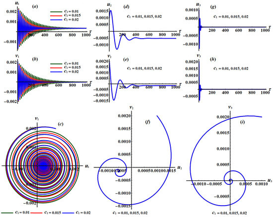
Figure 32. Time histories of $u_j\hspace{0.17em}\hspace{0.17em}(j=1,2,3)$ , $v_j$, and the projection of phase planes tracks $\hspace{0.17em}{u}_j{v}_j$ when $c_2=0.02,$ $c_3=0.2$, ${\omega }_1=3.354,$ and ${\omega }_2=3.131$: (a–i) at $c_1(=0.01,0.015,0.02)$.

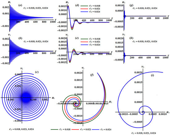
Figure 33. Time histories of $u_j\hspace{0.17em}\hspace{0.17em}(j=1,2,3)$, $v_j$, and the projection of phase planes tracks $\hspace{0.17em}{u}_j{v}_j$ when $c_1=0.01,$ $c_3=0.2$, ${\omega }_1=3.354,$ and ${\omega }_2=3.131$: (a–i) at $c_2(=0.018,0.021,0.024)$.

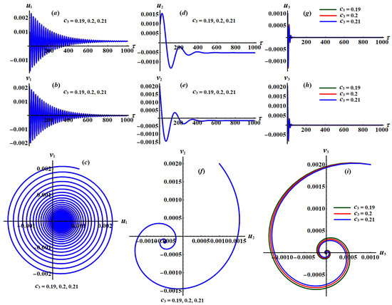
Figure 34. Time histories of $u_j\hspace{0.17em}\hspace{0.17em}(j=1,2,3)$, $v_j$, and the projection of phase planes tracks $\hspace{0.17em}{u}_j{v}_j$ when $c_1=0.01,$ $c_2=0.02$, ${\omega }_1=3.354,$ and ${\omega }_2=3.131$: (a–i) at $c_3(=0.19,0.2,0.21)$.

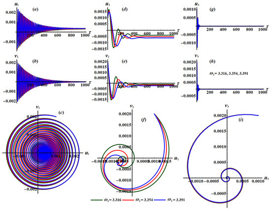
Figure 35. Time histories of $u_j\hspace{0.17em}\hspace{0.17em}(j=1,2,3)$, $v_j$, and the projection of phase planes tracks $\hspace{0.17em}{u}_j{v}_j$ when ${\omega }_2=3.131,$ $c_1=0.01,$ $c_2=0.02$, and $c_3=0.2$: (a–i) at ${\omega }_1(=3.316,3.354,3.391)$.

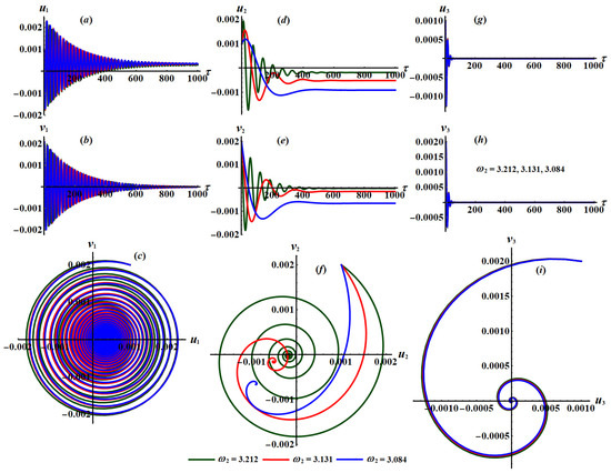
Figure 36. Time histories of $u_j\hspace{0.17em}\hspace{0.17em}(j=1,2,3)$, $v_j$, and the projection of phase planes tracks $\hspace{0.17em}{u}_j{v}_j$ when ${\omega }_1=3.354,$ $c_1=0.01,$ $c_2=0.02$, and $c_3=0.2$: (a–i) at ${\omega }_2(=3.212,3.131,3.084)$.

The time histories of the new modified phases $u_j$ and $v_j\hspace{0.17em}(j=1,2,3)$ are portrayed in parts (a), (d), and (g) and (b), (e), and (h) of Figure 32, Figure 33, Figure 34, Figure 35 and Figure 36, while parts (c), (f), and (i) show the projections of the trajectories of modulation equations on the phase planes $u_j{v}_j$. Figure 32, Figure 33 and Figure 34 are drawn at ${\omega }_1=3.354$ and ${\omega }_2=3.131$ when $c_1(=0.01,0.015,0.02),$ $c_2(=0.018,0.021,0.024),\hspace{0.17em}$ and $c_3(=0.19,0.2,0.21)$, respectively. Moreover, Figure 35 and Figure 36 are calculated at $c_1=0.01,$ $c_2=0.02,$ and $c_3=0.2$ when ${\omega }_1(=3.316,3.354,3.391)$ and ${\omega }_2(=3.212,3.131,3.084)$, respectively.

According to these figures, we can see a decaying manner in the trajectories of the waves characterizing $u_1,v_1,u_2,v_2$ and $u_3,v_3$ as drawn in parts (a), (b), (d), (e), (g), and (h) of Figure 32, Figure 33 and Figure 34 when $c_j\hspace{0.17em}(j=1,2,3)$ take various values, while the same conclusion for the mentioned parts can be found in Figure 35 and Figure 36 when ${\omega }_k\hspace{0.17em}(k=1,2)$ has distinct values. Moreover, the curves in planes $u_j{v}_j$, represented in parts (c), (f), and (i), behave as spiral curves and move toward a single point to confirm that the motion is free of chaos.

A closer look to Figure 32, Figure 33 and Figure 34 reveals that the new parameters $u_1$ and $v_1$ besides the phase plane curves $u_1{v}_1$ have been impacted with the change of $c_1$ more than the others values of $c_2$ and $c_3$. The time histories of $u_2,v_2$ and $u_3,v_3$ in addition to the curves of the planes $u_2{v}_2$ and $u_3{v}_3$ have been impacted with the change of the damping parameters $c_2$ and $c_3$, respectively. The principal reason goes back to the nature formulation of the system of equations (33). The spiral curves are directed from the outside to the inside, describing the stability of the studied system.

The good effectiveness of the change of the frequency parameters ${\omega }_1$ and ${\omega }_2$ on the dynamical behavior of considered system (33) has been shown in parts of Figure 35 and Figure 36. Time histories curves of the new parameters $u_j\hspace{0.17em}\hspace{0.17em}(j=1,2,3)$ and $v_j$ are plotted in parts (a), (d), and (g) and (b), (e), and (h), respectively. Whereas the plane curves $u_j{v}_j$ have been drawn in parts (c), (f), and (i) of Figure 35 and Figure 36. It is noted that these waves have been impacted with the various values of the frequency parameters, in which decay curves of the time histories are obtained and spiral ones of the phase plane toward one single point are plotted, indicating that the motion is smooth, steady and without disorder.

8. Conclusions

The non-linear motion of a damped spring pendulum with an attached linear damped transverse absorber in the direction of the spring has been investigated. Under the impact of a harmonic force and moment, the motion of the pendulum’s hanging point has been constrained to an elliptic path. The EOM have been derived applying Lagrange’s equations from the second kind. The AMS has been used to achieve the approximate solutions up to the third order. Based on the solvability requirements, the ME have been recognized. Three resonance cases of primary external and internal resonance were investigated simultaneously. The RHC was used to investigate and evaluate the stability of fixed points’ locations. The time histories of the achieved solutions, resonance responses, and the stability and instability zones at the steady state case were drawn and analyzed. The impact of various inputs of physical parameters on the performance of the system under investigation was examined. This system carries a lot of weight due to its use in engineering vibrational control applications.

References

- Thomson, W. Theory of Vibration with Applications, 5th ed.; Prentice Hall: Hoboken, NJ, USA, 1998. [Google Scholar]
- Wu, S. Active pendulum vibration absorbers with a spinning support. J. Sound Vib. 2009, 323, 1–16. [Google Scholar] [CrossRef]
- Eissa, M.; Kamel, M.; El-sayed, A.T. Vibration reduction of a nonlinear spring pendulum under multi external and parametric excitations via a longitudinal absorber. Meccanica 2011, 46, 325–340. [Google Scholar] [CrossRef]
- EL-Sayed, A.T.; Kamel, M.; Eissa, M. Vibration reduction of a pitch-roll ship model with longitudinal and transverse absorbers under multi excitations. Math. Comput. Model. 2010, 52, 1877–1898. [Google Scholar] [CrossRef]
- Eissa, M.; Kamel, M.; El-Sayed, A.T. Vibration reduction of multi-parametric excited spring pendulum via a transversally tuned absorber. Nonlinear Dyn. 2010, 61, 109–121. [Google Scholar] [CrossRef]
- Wu, S.; Siao, P. Auto-tuning of a two-degree-of-freedom rotational pendulum absorber. J. Sound Vib. 2012, 331, 3020–3034. [Google Scholar] [CrossRef]
- Nayfeh, H. Perturbation Methods; John Wiley & Sons: Hoboken, NJ, USA, 2008. [Google Scholar]
- Amer, W.S.; Bek, M.A.; Abohamer, M.K. On the motion of a pendulum attached with tuned absorber near resonances. Results Phys. 2018, 11, 291–301. [Google Scholar] [CrossRef]
- Amer, T.S.; Bek, M.A.; Hassan, S.S. Sherif Elbendary, The stability analysis for the motion of a nonlinear damped vibrating dynamical system with three-degrees-of-freedom. Results Phys. 2021, 28, 104561. [Google Scholar] [CrossRef]
- Awrejcewicz, J.; Starosta, R.; Kaminska, G. Asymptotic analysis of resonances in nonlinear vibrations of the 3-dof pendulum. Differ. Equ. Dyn. Syst. 2013, 21, 123–140. [Google Scholar] [CrossRef]
- Amer, T.S.; Bek, M.A. Chaotic responses of a harmonically excited spring pendulum moving in circular path. Nonlinear Anal. RWA 2009, 10, 3196–3202. [Google Scholar] [CrossRef]
- Starosta, R.; Kaminska, G.S.; Awrejcewicz, J. Parametric and external resonances in kinematically and externally excited nonlinear spring pendulum. Int. J. Bifurcat. Chaos 2011, 21, 3013–3021. [Google Scholar] [CrossRef]
- Starosta, R.; Kamińska, G.S.; Awrejcewicz, J. Asymptotic analysis of kinematically excited dynamical systems near resonances. Nonlinear Dyn. 2012, 68, 459–469. [Google Scholar] [CrossRef]
- El-Sabaa, F.M.; Amer, T.S.; Gad, H.M.; Bek, M.A. On the motion of a damped rigid body near resonances under the influence of harmonically external force and moments. Results Phys. 2020, 19, 103352. [Google Scholar] [CrossRef]
- Abady, I.M.; Amer, T.S.; Gad, H.M.; Bek, M.A. The asymptotic analysis and stability of 3DOF non-linear damped rigid body pendulum near resonance. Ain Shams Eng. J. 2021. [Google Scholar] [CrossRef]
- Amer, T.S.; Bek, M.A.; Abouhmr, M.K. On the vibrational analysis for the motion of a harmonically damped rigid body pendulum. Nonlinear Dyn. 2018, 91, 2485–2502. [Google Scholar] [CrossRef]
- Amer, T.S.; Bek, M.A.; Abohamer, M.K. On the motion of a harmonically excited damped spring pendulum in an elliptic path. Mech. Res. Commu. 2019, 95, 23–34. [Google Scholar] [CrossRef]
- Bek, M.A.; Amer, T.S.; Almahalawy, A.; Elameer, A.S. The asymptotic analysis for the motion of 3DOF dynamical system close to resonances. Alex. Eng. J. 2021, 60, 3539–3551. [Google Scholar] [CrossRef]
- Amer, T.S.; Bek, M.A.; Hassan, S.S. The dynamical analysis for the motion of a harmonically two degrees of freedom damped spring pendulum in an elliptic trajectory. Alex. Eng. J. 2021, 61, 1715–1733. [Google Scholar] [CrossRef]
- Tondl, A.; Nabergoj, R. Dynamic absorbers for an externally excited pendulum. J. Sound Vib. 2000, 234, 611–624. [Google Scholar] [CrossRef]
- Song, Y.; Sato, H.; Iwata, Y.; Komatsuzaki, T. The response of a dynamic vibration absorber system with a parametrically excited pendulum. J. Sound Vib. 2003, 259, 747–759. [Google Scholar] [CrossRef]
- Zhu, S.J.; Zheng, Y.F.; Fu, Y.M. Analysis of non-linear dynamics of a two-degree-of-freedom vibration system with non-linear damping and non-linear spring. J. Sound Vib. 2004, 27, 115–124. [Google Scholar] [CrossRef]
- Kecik, K.; Kapitaniak, M. Parametric analysis of magnetorheologically damped pendulum vibration absorber. Int. J. Struct. Stab. Dyn. 2014, 14, 1–13. [Google Scholar] [CrossRef]
- Kecik, K. Dynamics and control of an active pendulum system. Int. J. Non-Linear Mech. 2015, 70, 63–72. [Google Scholar] [CrossRef]
- Kecik, K. Assessment of energy harvesting and vibration mitigation of a pendulum dynamic absorber. Mech. Syst. Signal Process. 2018, 106, 198–209. [Google Scholar] [CrossRef]
- Kecik, K.; Mitura, A. Theoretical and experimental investigations of a pseudo-magnetic levitation system for energy harvesting. Sensors 2020, 20, 1623. [Google Scholar] [CrossRef] [PubMed] [Green Version]
- Kecik, K. Simultaneous vibration mitigation and energy harvesting from a pendulum-type absorber. Commun. Nonlinear Sci. Numer. Simulat. 2021, 92, 105479. [Google Scholar] [CrossRef]
- Djebali, S.; Aoun, A.G. Resonant fractional differential equations with multi-point boundary conditions on (0,+ꝏ). J. Nonlinear Funct. Anal. 2019, 2019, 1–15. [Google Scholar]
- Reich, S.; Zaslavski, A.J. Asymptotic behavior of a dynamical system on a metric space. J. Nonlinear Var. Anal. 2019, 3, 79–85. [Google Scholar]
- Awrejcewicz, J. Classical Mechanics: Kinematics and Statics; Springer: New York, NY, USA, 2012. [Google Scholar]
- Abohamer, M.K.; Awrejcewicz, J.; Starosta, R.; Amer, T.S.; Bek, M.A. Influence of the motion of a spring pendulum on energy-harvesting devices. Appl. Sci. 2021, 11, 8658. [Google Scholar] [CrossRef]
- Bek, M.A.; Amer, T.S.; Sirwah, M.A.; Awrejcewicz, J.; Arab, A.A. The vibrational motion of a spring pendulum in a fluid flow. Results Phys. 2020, 19, 103465. [Google Scholar] [CrossRef]
- Amer, T.S.; Galal, A.A.; Abolila, A.F. On the motion of a triple pendulum system under the influence of excitation force and torque. Kuwait J. Sci. 2021, 48, 1–17. [Google Scholar] [CrossRef]
- Amer, T.S.; Starosta, R.; Elameer, A.S.; Bek, M.A. Analyzing the stability for the motion of an unstretched double pendulum near resonance. Appl. Sci. 2021, 11, 9520. [Google Scholar] [CrossRef]
- Amer, W.S.; Amer, T.S.; Starosta, R.; Bek, M.A. Resonance in the cart-pendulum system-an asymptotic approach. Appl. Sci. 2021, 11, 11567. [Google Scholar] [CrossRef]
Publisher’s Note: MDPI stays neutral with regard to jurisdictional claims in published maps and institutional affiliations. |
© 2021 by the authors. Licensee MDPI, Basel, Switzerland. This article is an open access article distributed under the terms and conditions of the Creative Commons Attribution (CC BY) license (https://creativecommons.org/licenses/by/4.0/).