Memory Model for Morphological Semantics of Visual Stimuli Using Sparse Distributed Representation

Featured Application

Continual learning algorithm development in AI fields.

Abstract

Recent achievements on CNN (convolutional neural networks) and DNN (deep neural networks) researches provide a lot of practical applications on computer vision area. However, these approaches require construction of huge size of training data for learning process. This paper tries to find a way for continual learning which does not require prior high-cost training data construction by imitating a biological memory model. We employ SDR (sparse distributed representation) for information processing and semantic memory model, which is known as a representation model of firing patterns on neurons in neocortex area. This paper proposes a novel memory model to reflect remembrance of morphological semantics of visual input stimuli. The proposed memory model considers both memory process and recall process separately. First, memory process converts input visual stimuli to sparse distributed representation, and in this process, morphological semantic of input visual stimuli can be preserved. Next, recall process can be considered by comparing sparse distributed representation of new input visual stimulus and remembered sparse distributed representations. Superposition of sparse distributed representation is used to measure similarities. Experimental results using 10,000 images in MNIST (Modified National Institute of Standards and Technology) and Fashion-MNIST data sets show that the sparse distributed representation of the proposed model efficiently keeps morphological semantic of the input visual stimuli.

1. Introduction

Recent deep neural networks and learning algorithms show outstanding performance improvements. These results arise more affirmative expectations of future technological development [1,2,3]. On the other hand, these promising technologies also have quite a lot of limitations as well. Optimizing structure of deep neural networks and various hyper parameters as well as computing infra for highly complicated training algorithms are well known problems. In addition, the recent deep neural algorithms require huge volume of training data set with tag information and further almost algorithms support offline learning using the preconstructed training data set. Therefore, transition of problem domain or revision of training data set require new learning process from the beginning.

In general, training schemes for deep neural networks are different from biological learning method. As we all well understand, biological objects selectively receive and remember external stimuli input from sensory organs. We can consider biological objects always perform online learning in everyday life using these memory process.

As an alternative to overcome limitation of deep neural networks, tries to imitate biological learning are encouraged more and more. This paper considers the most representative 2 of these tries. The one is SPAUN (Semantic Pointer Architecture Unified Model) [4] and the other is HTM (Hierarchical Temporal Memory) [5,6].

SPAUN is a brain simulation model which consists of 2.5 million spiking neurons. Based on this model, we can simulate various brain operation such as recognition, memory, learning, and reasoning.

In addition, HTM employs modeling memory mechanism in neocortical region of biological brain system. HTM is a memory model with hierarchical structure, and it usually bases memory-prediction model in brain. Further, HTM is a cognitive model which can analyze and process time series variations of sequential input data. HTM can be applied to detect abnormal state of server or application and abnormal using of system. Basically, HTM converts input data to SDR (Sparse Distributed Representation) and processes SDR for analyzing and prediction. According to HTM model, SDR can be considered as the most representative data format processed by neocortical region of brain.

This paper proposes a memory and recall model for morphological semantics within visual stimuli using SDR of HTM model. Neocortical region in biological brain takes in charge of high level of information processing including abstraction and conceptualization for stimuli from the external environment. In addition, it supports memory and recall functions when required. In these whole processes, we can model operational mechanism of neurons on neocortical region using SDR operation.

The morphological sematic memory model proposed in this paper consists of two parts such as memory process for input stimuli and recall process for previous memory. First, memory process can be considered as a process to convert input visual stimuli to SDR type data. We can assume SDR as a neuron activation pattern in neocortical region in the abstraction and conceptualization processes for input visual stimuli. For the next recall process, we consider a detection process to find the most similar SDR pattern in the memory from the SDR pattern of the given visual stimulus.

This paper consists of 5 sections. In Section 2, we introduce backgrounds of this work and related research results. Section 3 explains structures of the proposed memory and recall model, and Section 4 presents experimental results for MNIST [7] and Fashion-MNIST [8] dataset. Finally, Section 5 discusses conclusions and future works.

2. Related Researches

This section presents overview and analysis of researches for transforming external stimulus into memory and recalling stored memory. We can consider these researches for memory model on both sides such as psychological and computing approaches. In psychology, memory means ability for acquiring and storing very complex and abstract knowledge such as algebra or geometry as well as simple information like ordinary events in our daily life. Therefore, we can consider memory is one of the most important elements for constructing self-identity as the most prominent aspect of human behavior. Memory models for computing-based approaches usually start from human brain researches. In this section, we provide overviews of HTM model and semantic folding model which imitate neocortical operation mechanism for processing external stimulus in our brain.

2.1. Cognitive Psychological Memory Researches

The initial example of classical memory experiment can be Ebbinghaus’ forgetting curve experiment since 1885, and this research initiates Bartlett’s memory experiment [9,10]. After that Atkinson and Shiffrin introduce multi-store model which classify memory into 3 groups including sensory memory, short-term memory, and long-term memory illustrated in Figure 1 [11].

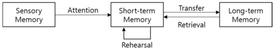
Figure 1. Atkinson and Shiffrin’s multi-store memory model which consists of sensory memory, short-term memory, and long-term memory [11].

Each storage space saves, processes, or forgets information when required. First, sensory memory stores input information from external environments, and it is known as keeping stored information during about 1 s. Next stage of memory is a short-term memory which perceive unforgotten information from sensory memory by attention. The short-term memory maintains stored information from a few seconds to 2 or 3 min. Even though memory time of short-term memory is longer than sensory memory, it begins to forget as well after a few minutes. We need repeated retrievals and rehearsals to maintain memory for a long time. As the last stage of memory, long-term memory is the place to store information passed by short-term memory for a long time. It is not clearly verified about its capacity and memory time.

Following the multi-store model, Baddeley introduced working memory instead of short-term memory [12]. In this research, he extends short-term memory and refer it to working memory, because most cognitive works about memorized information are performed in the short-term memory. According to Baddeley’s model, working memory consists of spatiotemporal information processing, voice and sound information processing, central processing unit, and a buffer for effective information processing. Figure 2 illustrates structure of Baddeley’s working memory model.

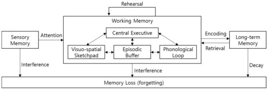
Figure 2. Alan Baddeley’s working memory model [12] with Atkinson and Shiffrin’s multi-store memory model [11].

This paper proposes a novel online learning scheme for consecutive input stimuli using memory models based on cognitive science.

2.2. Computing Models for Memory Mechanism

It is generally known that neocortical region of human brain is responsible for memories and high-level knowledge processing. This paper considers HTM as a simulation model for neuron activation mechanism in neocortical region of human brain.

Even though a neuron model in HTM is a simplified version of biological neuron and it is similar to the general artificial neuron model, we can consider it is more realistic than the neuron model of the existing artificial neural networks. Figure 3 shows neuron models of the existing artificial neural networks and HTM with a biological neuron model [13]. Figure 3a illustrates a biological neuron model, in which green lines mean proximal dendrites and blue lines mean distal dendrites. In addition, axons in a biological model have both feed-forward and lateral connections. On the other hand, the existing artificial neuron model shown in Figure 3b has only one kind of dendrite and axon with lateral connection. For HTM neuron model in Figure 3c, it has both proximal dendrite and distal dendrite like a biological neuron and axons with feed-forward connections as well as lateral connections.

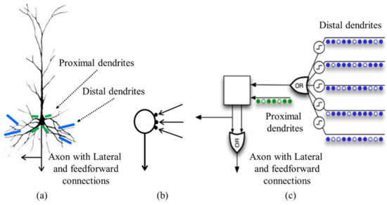
Figure 3. Comparison of (a) biological neuron, (b) artificial neuron model for the existing neural networks, and (c) a neuron cell model in HTM [13].

Visual information is processed through various regions in the neocortex of a biological brain as shown in Figure 4 [14]. Visual stimulus from the external environment is transferred through optic nerve into V1 region in the occipital lobe. V1 region processes visual features such as edges and lines from visual stimulus. Next, V2 region processes shape information using the edges and lines from V1 region. After that, shape information is used to find objects in V4 region and conceptual information such as faces in IT region. Thus, we can think low level visual feature is transformed into higher level information through abstraction and conceptual process.

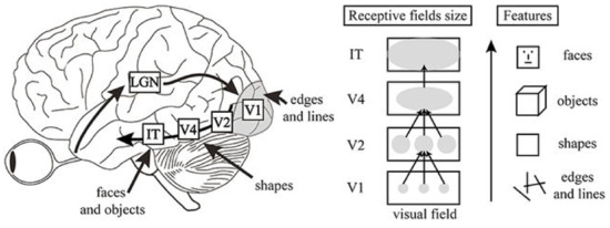
Figure 4. Visual information processing structure model in brain [14].

It is well known that every region of neocortex in human brain communicates information through the internal information delivery channel as shown in Figure 5a. Neocortex can be considered as thin sheet consisting multi-layered neurons. Each different region of thin neocortex sheet processes different information. Figure 5a illustrates 3 different visual cortex regions such as V1, V2, and V4. Visual sensory information fed into V1 is processed through many different regions with bi-directional connections on neocortex. Figure 5b shows one piece of neocortex sheet illustrating 6 layers of neurons and columnar structure. Each layer has its own number from 1 to 6. Layer 1 is the most outer layer and closer to brain surface. On the other hand, layer 6 is the most internal layer and closer to substantia alba.

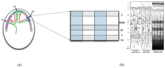
Figure 5. Structure of neocortex region of human brain [13,15]. (a) Visual cortex regions such as V1, V2, and V4, (b) A small part of vertical section of neocortex sheet.

Structure and operation of neurons in neocortex can be modeled using sparse distributed representation. It is because only a small part of neurons among huge number of neurons in neocortex is activated in a specific time. Sparse representation draws a great deal of attention because of its information embedding capacity. It can be used to find the most compact size of representation for the original data with underlying discriminative features. We can consider sparse graph research as a kind of sparse representation researches. Sparse graph can represent similarity weights between features. It can be used to improve the classification accuracy by the optimal feature selection [16,17,18]. In addition, sparse coding techniques are used for data compression, noise reduction, and interpolation, and so on. Sparse coding is developed to represent the original data using an overcomplete base vector [19,20,21].

SDR can embed huge amount of information by activating only a small number of neurons. In Equation (1), sparsity can be decided by ratio of activated neurons (w) to total neurons (n).

$$sparsity=\frac{w}{n}.$$

(1)

The capacity of SDR is defined by the volume of information in which SDR can embed, shown in Equation (2).

$$capacity=\left(\begin{array}{c}n\\ w\end{array}\right)=\frac{n!}{w!\left(n-w\right)!}.$$

(2)

For example, if total number of neurons is 16 and only 2 neurons are activated, sparsity of SDR can be decided as 0.125 and capacity of SDR is 120. If we increase total number of neurons to 256 and only 5 neurons of them are activated, sparsity is decreased to 0.0195 and capacity is considerably increased to 8,809,549,056. SDR examples of these 2 cases are illustrated in Figure 6.

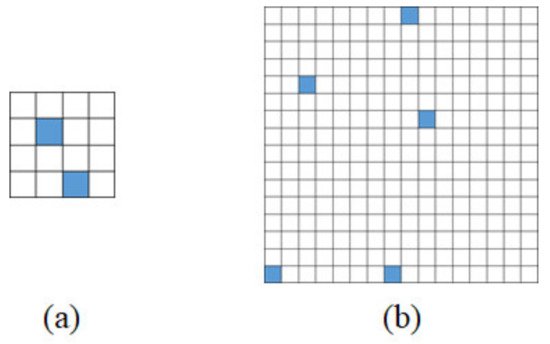
Figure 6. Examples of SDR according to total number of neurons and the number of activated neurons. (a) An example of only 2 activated neurons among 16 neurons, (b) An example of 5 activated neurons among.

Each cell of SDR which can embed such huge volume of information has feature for delivering somewhat meaningful information. Based on this feature, Cortical.IO proposes a method for folding semantic information using SDR [13,22]. According to Cortical.IO, semantic folding means the process for encoding words in a text document to sparse binary representation vector using distributed reference frame of semantic space. They provide it is possible to represent sentences or mutual semantic relations among words using semantic folding mechanism [22]. Figure 7 illustrates the concept of morphological semantic preservation scheme in this paper based on the idea of Cortical.IO. We can assume SDRs of images for number ‘0’, ‘5’, and ‘6’ have morphological similarities since these images have common round shapes. These morphological similarities can be found in the logical operation result of the 3 SDRs of images for number ‘0’, ‘5’, and ‘6’.

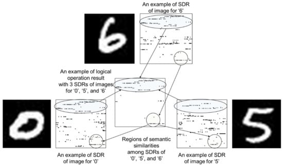
Figure 7. Concept of the proposed morphological semantic preservation scheme based on the idea of Cortical.IO. The regions of semantic similarities among SDRs of images ‘0’, ‘5’, and ‘6’ are indicated with circles.

3. Morphological Semantics Memory Model for Visual Stimuli

This section describes the proposed model with three concepts such as sensory memory, working memory, and long-term memory. This model provides a concise and precise description of the experimental results, their interpretation, as well as the experimental conclusions that can be drawn. This paper proposes a novel memory model to reflect remembrance of morphological semantics of visual input stimuli by combining the concepts of traditional cognitive and psychological memory models [11,12] and a neuron activation simulation model, that is, HTM [13]. The proposed model employs SDR for modeling interaction of neocortex in human brain which takes in charge of information processing and memory.

The general flow of the proposed memory model is illustrated in Figure 8. The proposed memory model is composed of three conceptual parts such as sensory memory, working memory, and long-term memory. First, the sensory memory part senses visual stimuli and extracts feature information from the sensed visual stimuli. Then, the working memory part converts the extracted feature information into SDR, known as a data representation pattern processed by a biological brain [5,6,13]. The working memory can also store input SDR as a new memory pattern, which corresponds to the consolidation process in cognitive psychology. And the working memory can also update the stored memory patterns through comparison operation with the previously stored memory patterns, which corresponds to the reconsolidation process in cognitive psychology. Finally, the long-term memory part defines what memories are stored and recalled, and it serves as the permanent storage of memories.

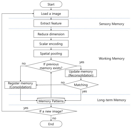
Figure 8. Memory model remembering the morphological semantics of visual stimuli.

3.1. Sensory Memory: Feature Extraction by CNN-Autoencoder

HTM neural model assumes that the operation of visual information processing in the brain is based on the activated pattern of neurons. Therefore, the features of a physical image must first be effectively extracted to convert an image into an activated pattern of neurons. Convolutional Neural Networks (CNN) [23] is widely used as an effective method for extracting image features in the field of machine learning. If features can be effectively extracted from physical images, it is easy to convert them to SDRs. Therefore, CNN-based technology is adopted in this model.

In addition, the supervised learning technique for feature extraction requires a high cost for constructing training data. Using unsupervised learning structure such as autoencoder [24] is beneficial to reduce this possible cost. Therefore, in this model, features are extracted from the image using a CNN-based autoencoder [25] that can effectively extract feature values with relatively low cost.

We believe that the better features in this stage make better results in the later steps, but the main purpose of this paper focuses on investigating memory and recall model based on a biological neuron activation scheme. For this reason, we employ a simple vanilla-level CNN-based autoencoder in this paper. In the implementation of the proposed memory model, the ground-truth label of the image is of no interest, but the ground-truth label of the data set is used in the experimental stage only for the performance evaluations.

Figure 9 shows the internal structure of the CNN-based autoencoder implemented to extract features from images. In this model, an autoencoder with three convolution layers with 16, 32, and 64, 3 × 3 filters respectively and two fully connected layers is used for feature extraction based on unsupervised learning. The extracted feature vector (Z) obtained by encoding part of the autoencoder is transferred to the working memory step, and additional data processing is performed for implementing memory model.

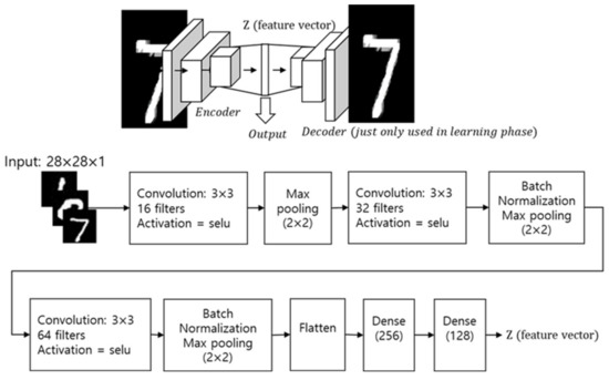
Figure 9. Feature extraction by CNN-autoencoder.

3.2. Working Memory: SDR Representation by Scalar Encoding and Spatial Pooling

The features extracted from physical images should be expressed in the way the brain processes them. According to a study on HTM and brain encoding [26,27], neural responses in the brain activated by external stimuli can be assumed to be blood flow patterns measured by functional magnetic resonance imaging (fMRI) from a macro perspective and sparsely distributed neural activation patterns from a micro perspective. In this implementation, the brain response to external visual stimuli is assumed to be a sparsely distributed neural activation pattern.

The first function of working memory is generating SDR representation. Figure 10 illustrates an internal data flow of an SDR encoder for converting a feature vector into an SDR. First, the SDR encoder adjusts the dimensions of the feature vector and then creates an SDR pattern through scalar encoding [28] and spatial pooling [29].

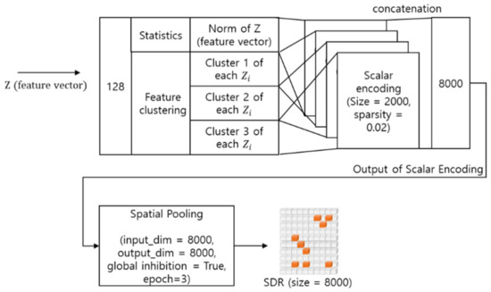
Figure 10. SDR representation process in SDR encoder.

In the dimension adjustment, the norm and distribution of the feature vector are extracted. Scalar encoding uses these values. Scalar encoding [28] converts a series of values into a bitstream, which corresponds to data preprocessing for spatial pooling. In scalar encoding parameters, size means the length of the converted bitstream, that is, the total number of bits. sparsity means the ratio of the number of active bits to the total number of bits. The set of values converted by scalar encoding is concatenated together to form a bitstream of a total of 8000 bits. These bits enter the input of spatial pooling.

Spatial pooling [29] converts the output of scalar encoding into a sparse distribution representation. Spatial pooling takes the binary output of a scalar encoding as input and assigns a finite number of columns to each input. Here, one column mimics a neuron column composed of several layers in the cerebral neocortex. In each column, a dendrite segment has a potential synapse that represents a subset of the input bits. Each potential synapse has a permanence value, and the state of the potential synapse may be changed to a connected synapse according to the permanence value. This process of spatial pooling can be expressed as shown in Figure 11.

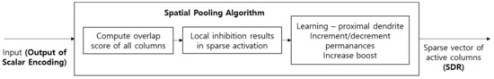
Figure 11. Processes for spatial pooling.

In spatial pooling, the number of activated synapses connected to each column is counted, and weights are considered to multiply by boost depending on the situation. In this case, the boost is determined according to how often the corresponding column is activated compared to the surrounding columns. In other words, if it is activated less often than the surrounding columns, the possibility of activation is increased by adjusting the boost to a larger value.

After this boost process, a certain volume of other columns within the inhibition radius is deactivated based on the largest formed column. In this case, the magnitude of the inhibition radius is dynamically adjusted according to the degree of diffusion of the input binary vectors. Through this process, a sparse set of active columns is determined.

In spatial pooling, the permanence of synapses connected to each active column can be adjusted. By increasing the permanence value of the synapse connected to the active input and decreasing the permanence value of the synapse connected to the inactive input, the synaptic connection can be changed to a valid or an invalid state.

3.3. Working Memory: Memory Operation by Consolidation and Reconsolidation

The second function of working memory is registering an SDR in case of a new input as a new memory pattern or recalling a stored memory pattern and updating it by fusion with the newly input SDR. Here, the registration process mimics the concept of consolidation in cognitive psychology and updating process mimics reconsolidation in cognitive psychology [30].

As shown in Figure 8, if there is no registered memory pattern, an input SDR is registered as a new memory pattern. However, when there are registered memory patterns, a similarity comparison between the input SDR and stored memory patterns is performed. At this time, the similarity is measured by the active bit overlap ratio between input SDR and stored memory patterns. If the active bit overlap ratio does not exceed a predefined threshold, the input SDR is also registered as a new pattern. In the current implementation, the newly registered memory pattern is just input SDR itself.

In other cases, if the active bit overlap ratio exceeds a predefined threshold, the input SDR and the stored memory pattern which has the highest overlap ratio make superposition SDR. Then, this superposition SDR is stored as an updated memory pattern.

There are things to consider when recalling the stored memory pattern. When a memory pattern is firstly registered, it is an SDR itself which has active bit intensity 1. However, as the input SDR and the stored memory pattern overlap through the update process, the active bit intensity of the stored memory pattern gradually increases. As a result, memory patterns with many updates have a wide distribution of active bits, and each active bit intensity is different. Therefore, it is necessary to determine at what level the stored memory pattern will be recalled in the process of loading the stored memory pattern to measure similarity with input SDR.

Figure 12 represents this concept as a picture, and the recall depth is automatically adjusted to maintain the sparsity of SDR when it is recalled.

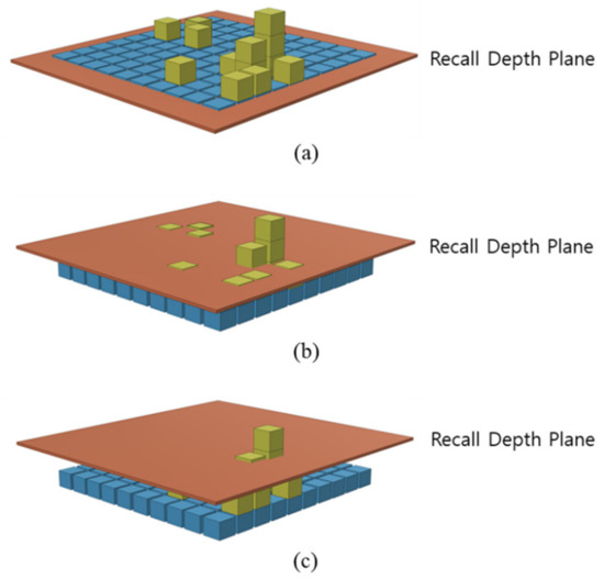
Figure 12. Recall depth plane: (a) All active bits participate in recall and reconsolidation operation, (b) Some of active bits participate in recall and reconsolidation, (c) Relatively high ranked active bits participate in recall and reconsolidation operation.

The advantage of this structure is that we can make comparisons with different precision of recall. For example, it provides a structure where you can ask questions such as ‘Is it a little similar?’, ‘Is it very similar?’ and ‘Is it the same?’

3.4. Long-Term Memory: Memory Definition

In cognitive psychology, stored memory is sometimes depicted as a schematic, a position to view memory from a macro perspective. From a neuroscientific point of view, stored memory can be interpreted as a stored pattern of activated neurons, which is a very microscopic perspective of memory. Connecting the two perspectives, memory can be seen as a pattern created by a group of activated neurons, and long-term memory can be seen as an autonomously enhanced nervous system pattern through biological phenomena such as synaptic enhancement or brainwave resonance. [31,32].

The format of ‘long-term memory’ in the memory model of this paper reflects the above point of view. Long-term memory is the superposition SDR of anecdotal visual stimulus SDRs that mimic the patterns of activated neurons, as shown in Figure 13.

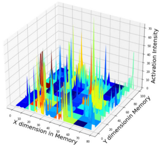
Figure 13. An example of long-term memory obtained from experiment and represented by superposition SDR; The location (x, y) axis of activated bits and its intensity z axis are embedding information about each memory pattern.

4. Experimental Results

The experiments are conducted in a desktop environment equipped with a GPU with TensorFlow 2.5 version installed in the python 3.7 execution environment.

To verify the memory model proposed in this paper, we have conducted two ways of experiments shown in Figure 14. The first experiment is conducted without prior memory as shown in Figure 14a. Whenever a new image is released, it is structured to generate and store new memories if the similarity level between memorized patterns is low, or to update the stored existing memories if the similarity level is high. In the experiment of (a), since the memory of morphological semantics matching the input image is not predetermined, many images tend to be created as new memories.

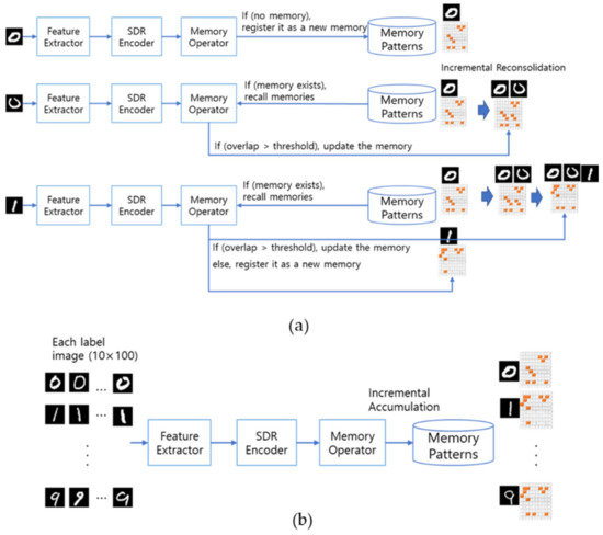
Figure 14. Experiment overview: (a) Procedures for generating progressive memories, (b) The process of creating a pre-memory.

Contrary to expectations, it is necessary to supplement the problem that morphologically similar images are formed by multiple memories. In the second experiment, we have conducted additional pre-memory process as shown in (b) by simulating that memory is effectively formed through the process of showing multiple picture cards in object recognition education for infants. In the pre-memory process, 100 images with high morphological similarity are continuously exposed to create an average pre-memory of morphological similarity in advance. After generating the prior memory in this way, the experiment in (a) is conducted to analyze the results.

4.1. Experiment 1: Memory Pattern Formation Experiment without Pre-Memory Process

The first experiment assumed that there is no initial memory of the image, and then sequentially entered the image one by one to form a memory. Images used for input are sequentially fed into the memory model with 10,000 test sets of the MNIST data set.

Figure 15 shows an example of a memory pattern formed when images are input one after another. When the label ‘7’ image is fed as the first input, it is registered as memory pattern 1 because there is no previously saved memory. When the label ‘2’ image is fed as the second input, the similarity is compared with the stored memory pattern 1, and since the similarity does not exceed the threshold, it is registered as a new memory pattern 2. This process repeats the above process whenever a new image comes in. When the label ‘1’ image comes in as the sixth image in the picture, the existing memory pattern 3 is updated because the similarity to the existing memory pattern 3 exceeds the criteria. The above process is iteratively performed for 10,000 test images.

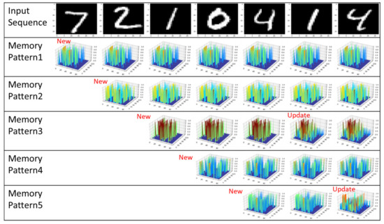
Figure 15. An example of forming an initial memory pattern without a pre-memory process.

Table 1 shows the number of generated memory patterns when SDR’s active bit overlap is applied as a similarity comparison criterion for image input of 10,000 test images and is visualized in Figure 16. The degree of overlap is varied from 20% to 60%, and if the SDR similarity does not exceed this ratio, it is saved as a new memory pattern. If the SDR overlap rate for judging the similarity is applied high, the image showing a slight difference is judged as a different memory pattern, and the memory pattern increases rapidly.

Table 1. Number of memory patterns compared to SDR overlapping rate.

Overlap Rate	100 Images	1000 Images	3000 Images	5000 Images	10,000 Images
20%	6	11	14	14	16
30%	10	17	22	25	29
40%	14	26	41	47	65
50%	27	55	85	97	122
60%	55	136	206	252	341

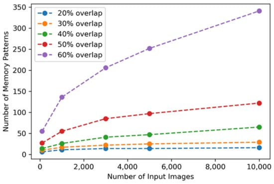
Figure 16. Number of memory patterns according to SDR overlapping ratio and number of input images without pre-memory process.

Each input image is converted into a unique SDR and then contributes to the update of the existing memory pattern or is registered as a new memory through similarity comparison with the stored memory pattern. As an example of the experimental results, when the similarity determination criterion is 20% active bit overlap, it is stored as 16 memory patterns when 10,000 test images are used. Since these figures exceed the expected range, additional analysis is conducted at the same time.

In Figure 17, when 16 memory patterns are stored, the distribution of labels belonging to each pattern is indicated by color codes. Here, the horizontal axis is the number of each memory pattern, and the vertical axis is the total number of images belonging to each memory pattern and the labels constituting it are indicated by color codes. Ideally, a small number of labels are included in a single memory pattern. Some memory patterns have a small number of labels, so it can be said that memory patterns are well formed according to morphological semantics, but there have been many cases where they are not.

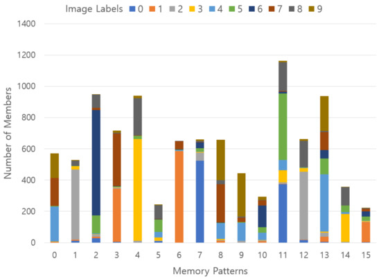
Figure 17. Results of stored memory pattern in an experiment using 20% SDR overlap without the pre-memory process; x-axis represents the memory patterns, y-axis describes the number of members belonging to each memory pattern, and a vertical color code indicates a ground-truth label ratio belonging to each memory pattern.

Figure 18 shows in which memory pattern the images of each label are distributed. Here, the horizontal axis represents the label number of the image used as an input, and the vertical axis represents the total number of each label and the ratio belonging to each memory pattern with 16 color codes. In the case of labels ‘3’ and ‘6’, it is judged that morphologically similar ones are relatively well patterned, but many labels are not stored in memory patterns according to morphological semantics. In other words, there should be a label indicating the dominant distribution in one memory pattern, but this distribution does not appear well and shows a mixed pattern.

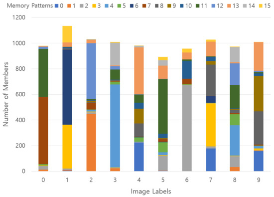
Figure 18. Results of stored memory pattern in an experiment using 20% SDR overlap without the pre-memory process; x-axis represents a ground-truth label, y-axis describes the number of members belonging to each label, and a vertical color code indicates a memory pattern ratio belonging to each ground-truth label.

As a result, there are some cases where a small number of images are stored as separate memories, and there are many cases where they are morphologically similar but stored as different memories. We can consider the main reason for these phenomena is initial memory problem. When forming a memory pattern while gradually feeding an image, if the data set has the same label but slightly different morphological feature, it is initially classified as a different memory. Therefore, in order to prevent such a problem, it is necessary to collect morphologically similar images in the beginning stage and perform pre-learning at once. The images of the data set used for the experiment show some morphological diversity even with the same label. However, it is necessary to assume that the ground-truth labels of the dataset are human-determined morphological similarities and create an average SDR of the images for each label and use it as a prior memory. In the second experiment, assuming that there is a prior memory, a new image is gradually fed to form a memory.

4.2. Experiment 2: Memory Pattern Formation Experiment Using Pre-Memory Process

In the second experiment, the need for prior memory is raised through the analysis of the results of the 4.1 experiment, and the pre-memory process is added to the introduction of the memory formation process. The pre-memory process simulates the fact that memory can be effectively formed by showing multiple picture cards in object recognition learning for young children. In the pre-memory process, images with high morphological similarity, that is, 100 images of the same label, are sequentially input to create an average pre-memory for morphological similarity in advance. After generating the prior memory in this way, the experiment in Section 4.1 is repeated and the results are analyzed.

First, let’s look at the memory patterns formed through pre-memory. Figure 19 illustrates the result of some memory patterns that formed the prior memory. These initial memory patterns of the picture are gradually updated according to a new input.

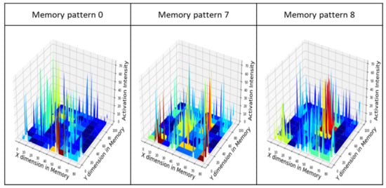
Figure 19. Examples of memory pattern formed through the pre-memory process.

Table 2 shows the number of generated memory patterns when SDR’s active bit overlap is applied to the remaining 9000 image inputs of the test set except for 1000 images used for pre-memory formation and is visualized in Figure 20. The overlap is applied while varying from 20% to 60%, and if the SDR similarity did not exceed this ratio, it is stored as a new memory pattern. In Experiment 1, if the SDR overlap for judging the similarity is applied high, the image showing a small difference is judged as a different memory pattern, resulting in a problem in which the memory pattern rapidly increased. However, in Experiment 2, when the pre-memory formation process is applied, the number of deviations from the pre-formed memory pattern gradually increased.

Table 2. Number of memory patterns compared to SDR overlapping rate.

Overlap Rate	100 Images	1000 Images	3000 Images	5000 Images	9000 Images
20%	10	10	10	10	10
30%	10	12	12	12	13
40%	15	18	24	24	33
50%	19	35	59	78	105
60%	44	96	148	199	286

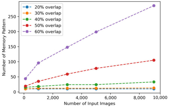
Figure 20. Number of memory patterns according to SDR overlapping ratio and number of input images with pre-memory process.

Each input image is converted into a unique SDR and then contributes to the update of the existing memory pattern or is registered as a new memory through similarity comparison with the stored memory pattern. As an example of the experimental result, when the similarity discrimination criterion is 20% active bit overlap, when the remaining 9000 images of the test set are used except for the 1000 images used for pre-memory formation, unlike Experiment 1, 10 memory patterns are stored. The number of stored memory patterns is equal to the number of ground-truth labels in the data set.

In Figure 21, when 10 memory patterns are stored, the distribution of labels belonging to each pattern is indicated by color codes. Here, the horizontal axis indicates the number of each memory pattern, and the vertical axis means the total number of images belonging to each memory pattern and the labels constituting it are indicated by color codes. Ideally, there should be only one label in one memory pattern, but there are many cases where the label indicating the majority distribution and the label of the minority distribution are mixed. This is because, when images are morphologically similar, different labels may appear together in one memory pattern.

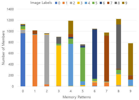
Figure 21. Results of stored memory pattern in an experiment using 20% SDR overlap with the pre-memory process; x-axis represents the memory patterns, y-axis describes the number of members belonging to each memory pattern, and a vertical color code indicates a ground-truth label ratio belonging to each memory pattern.

However, unlike Experiment 1, most of the memory patterns have labels indicating the dominant distribution, so it can be judged that the memory patterns are well formed according to the morphological semantics. Figure 22 shows which memory pattern the image of each label is saved. Here, the horizontal axis represents the label number of the image used as input, and the horizontal axis represents the total number of labels and the ratio belonging to each memory pattern with 10 color codes.

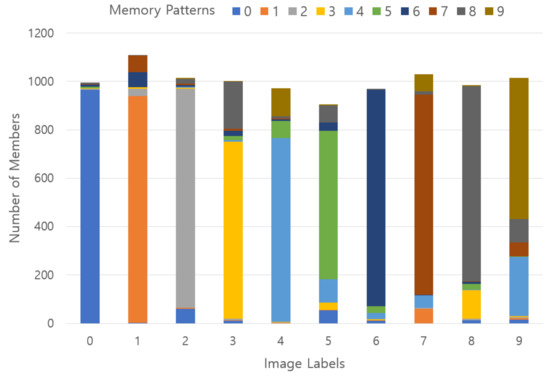
Figure 22. Results of stored memory pattern in an experiment using 20% SDR overlap with the pre-memory process; x-axis represents a ground-truth label, y-axis describes the number of members belonging to each label, and a vertical color code indicates a memory pattern ratio belonging to each ground-truth label.

4.3. Experiment 3: Memory Pattern Formation Experiment Using Pre-Memory Process for Fashion-MNIST Dataset

Experiment 3 are the same process of Experiment 2 using the Fashion-MNTST dataset and explained the results. What we want to check in Experiment 3 is to examine the extension of the proposed memory model. Experiment 3 uses a slightly more complex Fashion-MNIST dataset than the MNIST dataset. The Fashion-MNIST dataset is reconstructed by grouping morphologically similar images as shown in Figure 23. For example, t-shirt/top, pullover, coat, and shirt, which are similar in shape, were grouped into one class, and sneaker and ankle boot were grouped into another class, and input data was composed of a total of 6 classes and used.

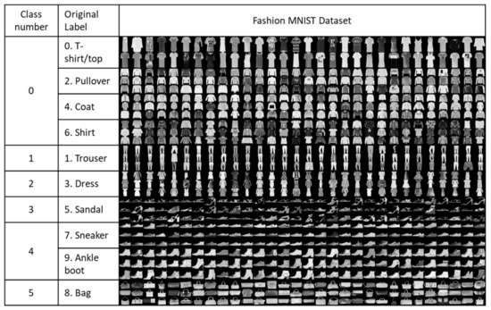
Figure 23. Fashion-MNIST dataset reclassed into morphologically similar image groups for experiments.

Figure 24 shows the result of converting Fashion-MNIST data composed of 6 classes into memory patterns. Class 0 representing t-shirt/top, pullover, coat, and shirt appears in memory pattern 0, class 1 representing trousers appears in memory pattern 2, and class 3 representing dress appears in memory pattern 2 at a relatively high ratio. In memory pattern 3, class 3 and class 4 are gathered in half, but sandals, sneakers, and ankle boots are gathered, so it can be considered that shoes are well remembered. Class 0 and class 5 are mainly gathered in memory pattern 5, which is believed to be because clothes and bags have similar shapes in the picture.

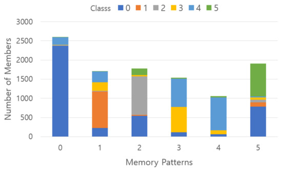
Figure 24. Results of stored memory pattern in an experiment using 20% SDR overlap with the pre-memory process for Fashion-MNIST dataset; x-axis represents class numbers, y-axis describes the number of members belonging to each memory pattern, and a vertical color code indicates a memory pattern ratio belonging to each class.

4.4. Discussions

Section 4.1 shows the experimental results of memory patterns generated when images are gradually input without generating prior memories, and Section 4.2 presents the experimental results of memory patterns generated when images are gradually input after pre-memory generation.

There are two main differences between results of Experiment 1 and Experiment 2. The first difference is that the number of memory patterns in Experiment 1 is greater than those in Experiment 2. In Experiment 1, a small difference in the image is recognized as another memory pattern and the number of memory patterns increased, when a memory pattern is created only with gradual image input without prior memory. In particular, the number of memory patterns is increased rapidly when high SDR overlap is applied based on similarity criteria. However, if memory patterns are created after pre-memory formation, fragmentation is reduced, and if SDR overlap is applied at 20%, the same number of memory patterns as the number of ground-truth labels are created.

The second difference is that it is much more difficult to find a dominant ground-truth label in Experiment 1. There are various ground-truth labels in a formed memory pattern when it is made only with gradual image input without prior memory. However, when a memory pattern is created after pre-memory formation, a dominant label appears in each memory pattern.

Figure 25 illustrates the comparison results with and without the pre-memory process when the 20% SDR overlap is used as the mutual similarity criterion. In this graph, the comparison values are the proportion of labels that appear dominant in each memory pattern. Meanwhile, the number of memory patterns differs when using and not using a pre-memory process. When the pre-memory process is used, 10 memory patterns are obtained, whereas 16 memory patterns are obtained when the pre-memory is not used. In order to compare the results under the same number of memory pattern conditions, 10 memory patterns containing many images out of 16 memory patterns were used.

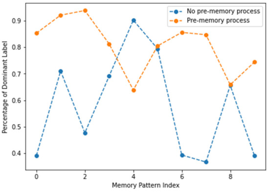
Figure 25. Comparison of the proportion of dominant labels with and without the pre-memory process. The similarity criterion is 20% SDR overlap.

Figure 26 illustrates the proportion of dominant memory pattern per ground-truth label according to the presence or absence of pre-memory when SDR 20% overlap is used as a similarity criterion. We can find that the proportion of the dominant memory pattern is very high in the result of the case where the pre-memory generation process is not performed compared to the result in the case where the pre-memory generation process is not performed.

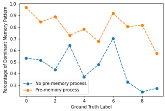
Figure 26. Percentage of dominant memory pattern for each ground-truth label in SDR 20% overlap as a similarity criterion.

5. Conclusions

This paper proposes a novel scheme for modeling memory mechanism in neocortical region of human brain. The proposed scheme models how visual stimuli has connected to memory system and how information in the memory system can be reconstructed during the recall process. We employ sparse distributed representation which imitates a neuron activation model in neocortical region of human brain for memory and recall process.

We have evaluated the proposed morphological semantic preservation scheme during memory and recall processes. In memory process, external visual stimuli are transformed to SDR from 128-dimension feature vector using encoder part of autoencoder based on CNN model. SDR pattern which represents memorized information from external stimuli can be considered to include semantic information. This paper considers morphological semantics especially. During the recall process, we detect the most similar memory with the given visual stimulus using similarity analysis in the SDR domain. This paper has used MNIST data set for the evaluation of effectiveness of the proposed scheme.

This paper can be considered as an inter-disciplinary research result. We have been tried to combine memory model from the viewpoint of behaviorism in the traditional cognitive psychology and visual information processing technology using neuron models from neuroscience. In this stage, we can consider 3 kinds of future research directions. The first is improvements of SDR mechanism for embedding semantic information more effectively in the memory process. This includes the fine tuning of feature vector selection scheme instead of vanilla level of autoencoder. The next is extending our scheme for 3-channel color image datasets, as well. After that, we are going to extend embedded information in SDR from morphological level to conceptual level. We consider knowledge construction process for conceptualization.

References

- Hinton, G.E.; Osindero, S.; Teh, Y.-W. A Fast Learning Algorithm for Deep Belief Nets. Neural Comput. 2006, 18, 1527–1554. [Google Scholar] [CrossRef] [PubMed]
- LeCun, Y.; Bengio, Y.; Hinton, G. Deep learning. Nature 2015, 521, 436–444. [Google Scholar] [CrossRef] [PubMed]
- Goodfellow, I.; Pouget-Abadie, J.; Mirza, M.; Xu, B.; Warde-Farley, D.; Ozair, S.; Courville, A.; Bengio, Y. Generative adversarial nets. Adv. Neural Inf. Process. Syst. 2014, 27, 2672–2680. [Google Scholar]
- Eliasmith, C. How to Build a Brain: A Neural Architecture for Biological Cognition; Oxford Series on Cognitive Models and Architectures; Oxford University Press: Oxford, UK, 2013. [Google Scholar]
- Ahmad, S.; George, D.; Edwards, J.L.; Saphir, W.C.; Astier, F.; Marianetti, R. Hierarchical Temporal Memory (HTM) System Deployed as Web Service. U.S. Patent US20170180515A1, 20 May 2014. [Google Scholar]
- Hawkins, J.; Blakeslee, S. On Intelligence: How a New Understanding of the Brain Will Lead to the Creation of Truly Intelligent Machines; St. Martin’s Griffin, Macmillan: New York, NY, USA, 2007. [Google Scholar]
- Deng, L. The MNIST Database of Handwritten Digit Images for Machine Learning Research. IEEE Signal Process. Mag. 2012, 29, 141–142. [Google Scholar] [CrossRef]
- Xiao, H.; Rasul, K.; Vollgraf, R. Fashion-MNIST: A Novel Image Dataset for Benchmarking Machine Learning Algorithms. arXiv 2017, arXiv:1708.07747. [Google Scholar]
- Ebbinghaus, H. Memory: A Contribution to Experimental Psychology. Ann. Neurosci. 2013, 20, 155–156. [Google Scholar] [CrossRef] [PubMed]
- Bartlett, F.C.; Burt, C. Remembering: A Study in Experimental and Social Psychology; Cambridge University Press: Cambridge, UK, 1932. [Google Scholar]
- Atkinson, R.C.; Shiffrin, R.M. Chapter: Human memory: A proposed system and its control processes. In The Psychology of Learning and Motivation; Spence, K.W., Spence, J.T., Eds.; Academic Press: New York, NY, USA, 1968; Volume 2, pp. 89–195. [Google Scholar]
- Baddeley & Hitch (1974)—Working Memory—Psychology Unlocked. 10 January 2017. Archived from the original on 6 January 2020. Retrieved 11 January 2017. Available online: http://www.psychologyunlocked.com/working-memory (accessed on 13 November 2021).
- Numenta, Hierarchical Temporal Memory Including HTM Cortical Learning Algorithms. 2011. Available online: https://numenta.com/assets/pdf/whitepapers/hierarchical-temporal-memory-cortical-learning-algorithm-0.2.1-en.pdf (accessed on 13 November 2021).
- Herzog, M.H.; Clarke, A.M. Why vision is not both hierarchical and feedforward. Front. Comput. Neurosci. 2014, 8, 135. [Google Scholar] [CrossRef] [PubMed][Green Version]
- George, D.; Hawkins, J. Towards a Mathematical Theory of Cortical Micro-circuits. PLoS Comput. Biol. 2009, 5, e1000532. [Google Scholar] [CrossRef] [PubMed]
- Hijazi, S.; Hoang, V.T. A Constrained Feature Selection Approach Based on Feature Clustering and Hypothesis Margin Maximization. Comput. Intell. Neurosci. 2021, 2021, 1–18. [Google Scholar] [CrossRef]
- Huang, X.; Zhang, L.; Wang, B.; Zhang, Z.; Li, F. Feature weight estimation based on dynamic representation and neighbor sparse reconstruction. Pattern Recognit. 2018, 81, 388–403. [Google Scholar] [CrossRef]
- Zhu, Y.; Zhang, X.; Wang, R.; Zheng, W.; Zhu, Y. Self-representation and PCA embedding for unsupervised feature selection. World Wide Web 2018, 21, 1675–1688. [Google Scholar] [CrossRef]
- Olshausen, B.A.; Field, D.J. Emergence of simple-cell receptive field properties by learning a sparse code for natural images. Nature 1996, 381, 607–609. [Google Scholar] [CrossRef] [PubMed]
- Sun, Z.; Yu, Y. Fast Approximation for Sparse Coding with Applications to Object Recognition. Sensors 2021, 21, 1442. [Google Scholar] [CrossRef] [PubMed]
- Zheng, H.; Yong, H.; Zhang, L. Deep Convolutional Dictionary Learning for Image Denoising. In Proceedings of the 2021 IEEE/CVF Conference on Computer Vision and Pattern Recognition (CVPR), Virtual, 19–25 June 2021; pp. 630–641. [Google Scholar]
- Webber, F. Semantic Folding Theory-White Paper; Cortical.IO. 2015. Available online: https://www.cortical.io/static/downloads/semantic-folding-theory-white-paper.pdf (accessed on 13 November 2021).
- LeCun, Y.; Kavukcuoglu, K.; Farabet, C. Convolutional networks and applications in vision. In Proceedings of the 2010 IEEE International Symposium on Circuits and Systems, Paris, France, 30 May–2 June 2010; IEEE: Piscataway, NJ, USA, 2010; pp. 253–256. [Google Scholar] [CrossRef]
- Baldi, P. Autoencoders, unsupervised learning, and deep architectures. J. Mach. Learn. Res. 2012, 27, 37–50. [Google Scholar]
- Boutarfass, S.; Besserer, B. Convolutional Autoencoder for Discriminating Handwriting Styles. In Proceedings of the 2019 8th European Workshop on Visual Information Processing (EUVIP), Roma, Italy, 28–31 October 2019; pp. 199–204. [Google Scholar] [CrossRef]
- Numenta. Sparsity Enables 100x Performance Acceleration in Deep Learning Networks; Technical Demonstration. 2021. Available online: https://numenta.com/assets/pdf/research-publications/papers/Sparsity-Enables-100x-Performance-Acceleration-Deep-Learning-Networks.pdf (accessed on 13 November 2021).
- Cui, Y.; Surpur, C.; Ahmad, S.; Hawkins, J. A comparative study of HTM and other neural network models for online sequence learning with streaming data. In Proceedings of the 2016 International Joint Conference on Neural Networks (IJCNN), Vancouver, BC, Canada, 24–29 July 2016; pp. 1530–1538. [Google Scholar] [CrossRef]
- Smith, K. Brain decoding: Reading minds. Nature 2013, 502, 428–430. [Google Scholar] [CrossRef] [PubMed]
- Purdy, S. Encoding Data for HTM Systems. Available online: https://arxiv.org/ftp/arxiv/papers/1602/1602.05925.pdf (accessed on 13 November 2021).
- Mnatzaganian, J.; Fokoué, E.; Kudithipudi, D. A Mathematical Formalization of Hierarchical Temporal Memory Cortical Learning Algorithm’s Spatial Pooler. 2016. Available online: http://arxiv.org/abs/1601.06116 (accessed on 13 November 2021).
- McKenzie, S.; Eichenbaum, H. Consolidation and Reconsolidation: Two Lives of Memories? Neuron 2011, 71, 224–233. [Google Scholar] [CrossRef] [PubMed]
- Goyal, A.; Miller, J.; Qasim, S.E.; Watrous, A.J.; Zhang, H.; Stein, J.M.; Inman, C.S.; Gross, R.E.; Willie, J.T.; Lega, B.; et al. Functionally distinct high and low theta oscillations in the human hippocampus. Nat. Commun. 2020, 11, 1–10. [Google Scholar] [CrossRef] [PubMed]
Publisher’s Note: MDPI stays neutral with regard to jurisdictional claims in published maps and institutional affiliations. |
© 2021 by the authors. Licensee MDPI, Basel, Switzerland. This article is an open access article distributed under the terms and conditions of the Creative Commons Attribution (CC BY) license (https://creativecommons.org/licenses/by/4.0/).