Featured Application
Advanced Driver Assistance Systems (ADAS).
Abstract
One of the main actions of the driver is to keep the vehicle in a road lane within its markings, which could be aided with modern driver-assistance systems. Forward digital cameras in vehicles allow deploying computer vision strategies to extract the road recognition characteristics in real-time to support several features, such as lane departure warning, lane-keeping assist, and traffic recognition signals. Therefore, the road lane marking needs to be recognized through computer vision strategies providing the functionalities to decide on the vehicle’s drivability. This investigation presents a modular architecture to support algorithms and strategies for lane recognition, with three principal layers defined as pre-processing, processing, and post-processing. The lane-marking recognition is performed through statistical methods, such as buffering and RANSAC (RANdom SAmple Consensus), which selects only objects of interest to detect and recognize the lane markings. This methodology could be extended and deployed to detect and recognize any other road objects.
1. Introduction
Modern automobiles have systematically incorporated new technologies, particularly associated with electronic devices and computational systems. The increasing complexity of automotive systems allows new supporting features of driver assistance systems (DAS) that improve performance, comfort, and safety [1,2]. The deployment of DAS features has been boosted by developing new integrated circuits, sensors, and actuators, which allowed intelligent devices, robust video processing techniques to recognize objects, and other high-performance technologies [3]. Some of those technologies have been a matter of technological differentiation for commercialization in the vehicle business. Nowadays, many of those technologies, such as airbags, Electronic Stability Control (ESC) system, and Antilock Brake System (ABS), are mandatory in cars manufactured in most countries.
In the USA, about 94% of traffic accidents are caused by driver failure [4]. The insertion of new features based on DAS could considerably reduce accidents in the cases of a rear collision, lane marking departure, improper lane marking changes, and over the limit speed [5]. Those elements represent a significant motivation for industry and academies to develop DAS features in commercial vehicles.
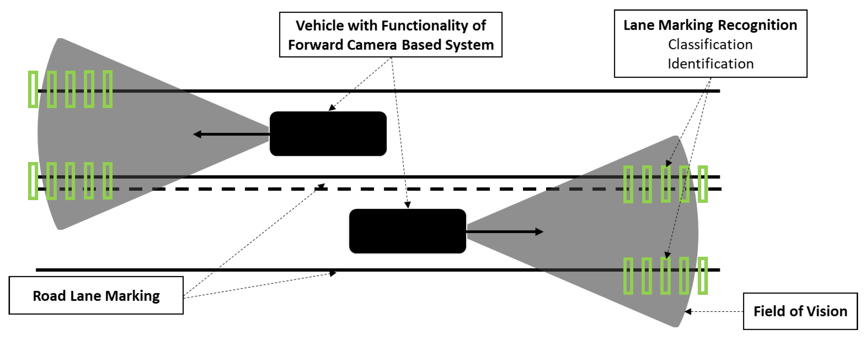
One of the main tasks for the drivers is to keep the vehicle within the lane markings, which considerably reduces the probability of accidents. Digital camera systems could help drivers capture road images and process them to recognize objects. Figure 1 shows the range of sight for a forward camera system in the vehicle, sensing the lane markings in the road and other objects in its field of vision.
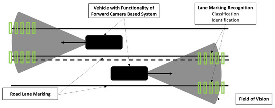
Figure 1.
Upper view of the digital camera’s range to recognize the lane markings on the road.
A front camera system in the vehicle captures real-time images of the vehicle’s surroundings. The acquired images are transferred to an onboard computational system that processes algorithms to recognize road elements such as lane markings, vehicles, pedestrians, and other obstacles, enabling driver assistance functionalities such as line departure warnings to the driver or taking action. For example, the process of lane marking recognition is performed by video processing techniques, which should identify and classify the road lane marking to deploy in-vehicle features to keep it on the lane. The most known features that demand lane-marking recognition are Lane Departure Warning (LDW) and Lane-Keeping Assist (LKA).
This work proposes a computational architecture to deliver satisfactory results in harsh environments, keeping a simple hardware setup, reducing costs, as compared to other proposed methodologies [6,7,8] based on sensor fusion and multimodal approaches. These harsh environments result from weather conditions, which introduce noise and disturbances in the visual perception system. We have developed a flexible and modular workflow that enables us to apply several techniques to recognize road lane marking. Moreover, we have established processing techniques that allowed buffering strategies and the RANdom SAmple Consensus (RANSAC) algorithm, which considerably improved lane marking detection. We confirmed the improvements of our method by a statistical verification method. In addition, we provide a dataset that may be checked to ensure the performance of our approach. Finally, the proposed strategy is not limited to lane marking recognition, being extensible to recognizing other road objects.
RANSAC Method for Lane Marking Recognition
The LDW system aims to prevent vehicles from leaving their respective lanes and causing accidents. We might calculate the road’s central medium line and threshold to serve as the reference by recognizing the lane marking. The gravity center of the vehicle should track the reference to let it drive safely. If the vehicle leaves the threshold, this could mean that the vehicle is in an unsafe condition, so the alert system can activate a warning message or even command the steering system to bring the vehicle back to a safe position. This work proposed the Random Sample Consensus (RANSAC) algorithm and other computer vision techniques to implement line marking recognition. To demonstrate the efficiency of the proposed algorithm, six different cases of variation in track lane marking are presented, as well as different drift variations.
A recent investigation presented a lane marking recognition using the Hough Transform method [9], adopting the near and far-field concept in the captured image. This technique for LDW activation can be implemented in conjunction with lane marking tracking using RANSAC. Another investigation explored track identification using inverse perspective projection along with RANSAC and the Kalman filter application [10].
Fangfang et al. [11] proposed the multiple-track identification by linking the inverse perspective transformation, Hough transform, and a RANSAC code. Kang et al. [12] applied Fangfang’s method to implement a low-cost driver-assistance system consisting of two functions. The first function applies the Modified Extended Census Transformation and carries out the vehicle identification through classification. The second function consists of noise attenuation and application of the RANSAC code to identify lane markings. A robust ego-lane marking track detection system based on the stages of lane marking segmentation, recognition, and estimation through the RANSAC algorithm was proposed [13] to facilitate the implementation on real-time computing platforms. Reference [14] demonstrated a lane marking detection system through the modified RANSAC code merged with the least-squares method. Additionally, an algorithm emphasizing robustness and efficiency, considering the RANSAC application with the hyperbolic model, was presented [15].
A lane marking detection system has been proposed using the application of small detection windows throughout the region of interest (ROI) [16] to binarize the image only in the windows that cover the behavior of the tracks. For the binarization process, the Otsu threshold method [17] with a preset threshold value of 50 ensured better border extraction and lower noise acquisition than the widely used Canny method [18]. Following the binarization process, the ROI was dived in the left and right parts for the application of RANSAC. This technique was applied in several climatic conditions and resulted in robust and reliable results.
This paper is organized in the following structure: Section 2 describes the proposed architecture, labeled ROADLANE, which supports algorithms and strategies for road lane marking recognition. The architecture comprises three main layers from bottom to top (from the digital camera up to features): pre-processing, processing, and post-processing. Section 3 shows the pre-processing stages with several handlers to deal with the image acquisition from a digital camera. Section 4 shows the processing with the RANSAC method to extract the road lane identification and Section 5 shows the post-processing. Section 6 shows the results and discussions of six cases, considering a sample of over 4000 frames of our GSA (Grupo de Sistemas Automotivos—Automotive Systems Group) database. The selected samples present different climatic scenarios and road scenarios. It shows how the entire process is integrated to obtain an LDW feature. Finally, Section 7 presents the conclusion.
2. Architecture to Support Algorithms and Strategies of Road Lane Marking Recognition
The ROADLANE is a modular architecture of object recognition designed to identify and recognize road lane markings. In addition, it enables the customization of the strategies and algorithms, complying with automotive requirements. Therefore, it can be used to provide additional functionalities to the advanced driver assistance system (ADAS) for safety and comfortable driving, such as lane departure warning, lane-keeping assistance, adaptive cruise control, and automated brake assistance.
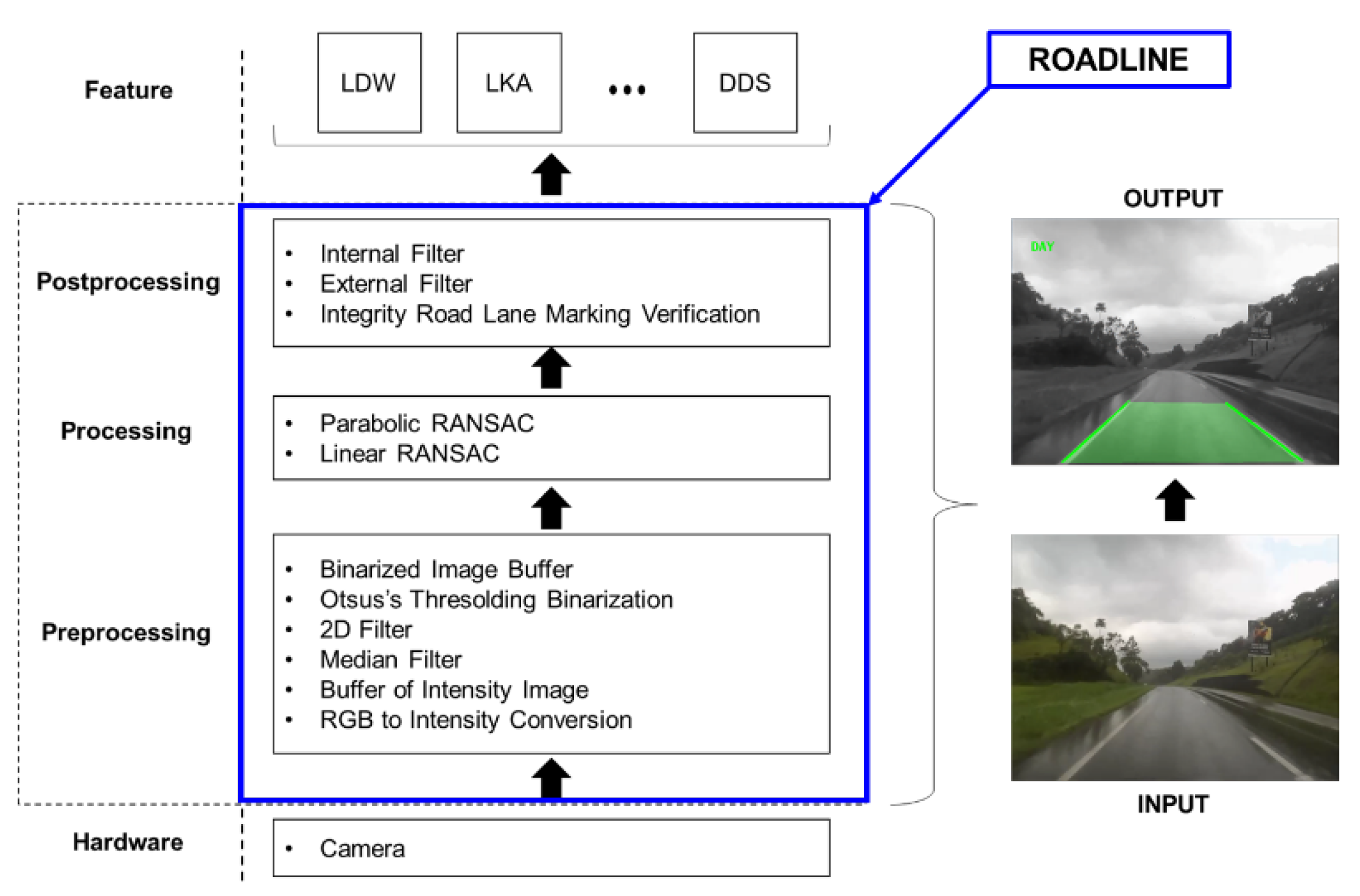
The proposed architecture comprises three main layers, or stages, where the image signal processing identifies and recognizes patterns, such as road lanes, vehicles, and pedestrians. The processing flow is carried out from the bottom to the top. The following three stages are defined: (1) pre-processing, (2) processing, and (3) post-processing, as shown in Figure 2. A digital camera acquires the road image, which is in the lower level of the architecture. The features that use the image processed are on the upper level. As mentioned in the previous paragraph, these are the functions of our interest. The right side of Figure 2 shows the input image from the digital camera, without processing, and the output image with added information regarding the object detection over the image, delivering features necessary to implement the desired functionality such as LDW, LKA, and Driver Drowsiness System (DDS).

Figure 2.
The ROADLANE architecture for road lane marking recognition.
The modular architecture provides the developer with the freedom to choose the algorithms, giving more flexibility. In addition, the contribution of this approach is the capability to adapt the statistical method with RANSAC to ensure a verification to deliver a lane marking recognition. In the proposed architecture, each layer has the following responsibilities:
- Pre-processing: primary operations, such as noise reduction, contrast enhancement, and sharpness.
- Processing: information extracted from the image, such as edges, contours, and identified objects), and
- Post-processing: electronic interpretation set of objects identified by cognitive functions usually associated with vision, as with computer vision [19,20].
The camera must be fixed inside the vehicle (Figure 3a) and positioned on the windshield’s upper left, coupled with the rearview mirror (Figure 3b). The camera’s resolution can be from 320 × 240 to 1200 × 1080 pixels, depending on the requirements of the target application. We consider that there is a tradeoff between resolution and FOV, which we defined the default setup with 1200 × 1080 pixels in fixed focus. This is sufficient to extract all the features of the image and video in data acquisition to be pre-processed. This is our strategy in calibration and use of the camera. The road environment image data captured by the frontal vehicle camera is streamed in real-time to an onboard vehicle computer and processed by ROADLINE architecture. The output of ROADLANE provides data for DAS applications with the objects of interest identified and classified, leaving it to the designer to specify the configuration according to the desired functionality.
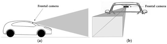
Figure 3.
(a) Positioning the camera sideways; (b) front camera positioning.
The front camera-based system is used in road vehicles to provide the functionalities related to the DAS, which can analyze the image content and extract features of interest. Our target example is the LKA, a feature that can assist the driver in keeping the vehicle within a lane by pushing it back by turning the steering wheel. It is effective because when the system verifies whether the vehicle is in the lane departure, the electronic steering unit can control the vehicle back to the correct position on the lane. If the steering pushback is not enough, the LKA function warns the driver to regain vehicle control. Figure 4 depicts the operation scenario of LKA and the reaction device that is activated to move the vehicle back into the lane.
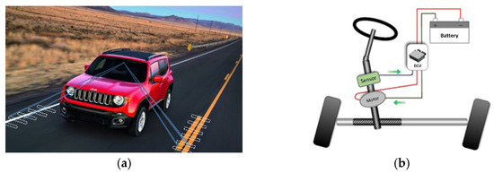
Figure 4.
(a) For LKA function, the input is the image captured by the camera, and calculation of lane and vehicle positions; (b) if the vehicle gets out of the lane boundary, an Electronic Power Steering (EPS) system is activated to keep the vehicle within the lane.
3. Pre-Processing
The pre-processing stage consists of the image acquisition from the camera in the RGB format. Next, feature extraction is performed to provide the upper stage of processing an image artifact only with the region of interest, which contains the road lane marking already filtered, binarized, and with edges detected. The following steps were taken in sequence: RGB to intensity conversion, buffering of intensity image, median filter, 2D filter, Otsu’s thresholding, and binary buffer. This stage must remove noises that affect the image, such as the windscreen wiper when it is in operation. The binary buffering process allows removing this type of noise.
It is essential to perform the image conversion from RGB to grayscale format. Therefore, the input frame or image in RGB format consists of a set of pixels, represented by a three-dimensional matrix that comprised indexes of the R (red), G (green), and B (black). After conversion to grayscale, it turns into a one-dimension matrix, that usually goes from 0 to 255 (0 = black and 255 = white) [19].
3.1. RGB to Grayscale
The camera acquires images of the road characteristics, providing the functionality of video acquisition in real-time, consisting of × frames/sec, in which a frame is a collection of pixels available in RGB format [21]. Therefore, the acquired frame represents the image of the road according to the field of vision of a camera. Therefore, the calibration and fixed focus configuration are necessary assignments. In addition, the image acquired may have noise, which can be removed based on applying the binary buffering technique over the grayscale image.
The conversion from RGB to grayscale or intensity is one of the first steps of image processing algorithms, reducing the amount of image information. It allows us to reduce the processing demand, while keeping the POI (Point of Interest) features in the image, and process the object recognition strategy faster. In addition, the ROI (Region of Interest) adoption provides effective process demands for just the specific region of interest, which in our case is the lane recognition. This conversion defines specific weights that must be applied to R, G, and B channels. Although a grayscale image contains less information than an RGB one, most essential features are maintained, such as edges.
The RGB to intensity conversion consists of the concatenation of three channels of a pixel, based on the multiplication of each channel by a specific factor and summed, to result in a single channel pixel. The conversion process keeps the dimensions of rows and columns of the frame and decreases the dimensions of each pixel from three to one. The multiplication factors based on the NTSC CCIR 601 standard are demonstrated in Equation (1) according to [20]. For , it means the specific pixel value in the image frame with index and [22], is obtained by using the following formula
where R, G, and B are color channel values corresponding respectively to red, green, and blue (R: Red, G: Green; and B: Blue). For the grayscale image, we still have a sharp image of the ROI. Nevertheless, the image output in grayscale enables an edge detection filter to be applied later. The edge detection allows characterizing and highlighting the objects contained in the image. There are several edge detection filters, such as Canny, Deriche, Sobel, and Prewitt.
Overall, the image in grayscale is an artifact to be delivered to perform the buffering method at the pixel level to remove undesirable noises [22].
Buffering of Grayscale Image
We consider that a vehicle has a windscreen wiper and a camera installed inside it. Therefore, the wiper operation is considered as noise for the image acquired by the camera. In this operation case, the windscreen wiper image appears so that it is not possible to see or estimate the image across the windscreen wiper. Therefore, we proposed to apply the buffering of the image to reduce the noise generated by the windscreen wiper.
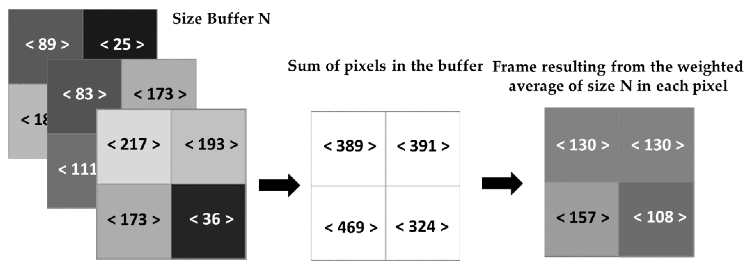
The process of buffering an image (Figure 5) that is already in grayscale consists of acquiring frames according to the size of the buffer (input), and the output frame consists of the weighted average of pixels of all the frames stored in the buffer. For each algorithm interaction, the oldest frame is removed, and the current one is added. Indeed, we define several frames to be buffered denoted by N, calculate the sum of each pixel intensity value in grayscale, and divide by N. The average of that specific pixel provides a new pixel that contains an entire image with removed noise. For example, Figure 5 shows three frames (N = 3) and three pixels, respectively, with values of 25, 173, and 193, with an average value of 130.
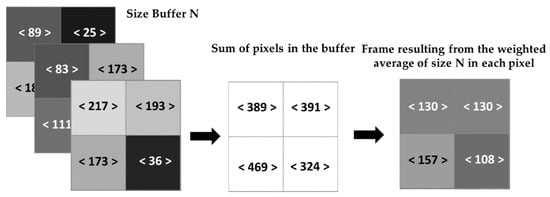
Figure 5.
The process of buffering the intensity image.
Through the buffering of the intensity, it is possible to reduce the noise. Depending on the vehicle speed, this process can attenuate or smooth some noises contained in the image. For example, this step can decrease the noise caused by the windscreen wiper (Figure 6).
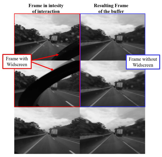
Figure 6.
Attenuation of noise with image buffering in grayscale.
We can establish the process to cut the image without noise and maintain only a specific ROI for the image without noise. The ROI is defined by the image region below the vanishing point for our application, which comprises the road lane we wish to identify and recognize. Therefore, the ROI can be cropped after applying the buffering method to reduce memory and processing. Indeed, the next step to apply the median filter is made only in the cropped ROI.
3.2. Median Filter
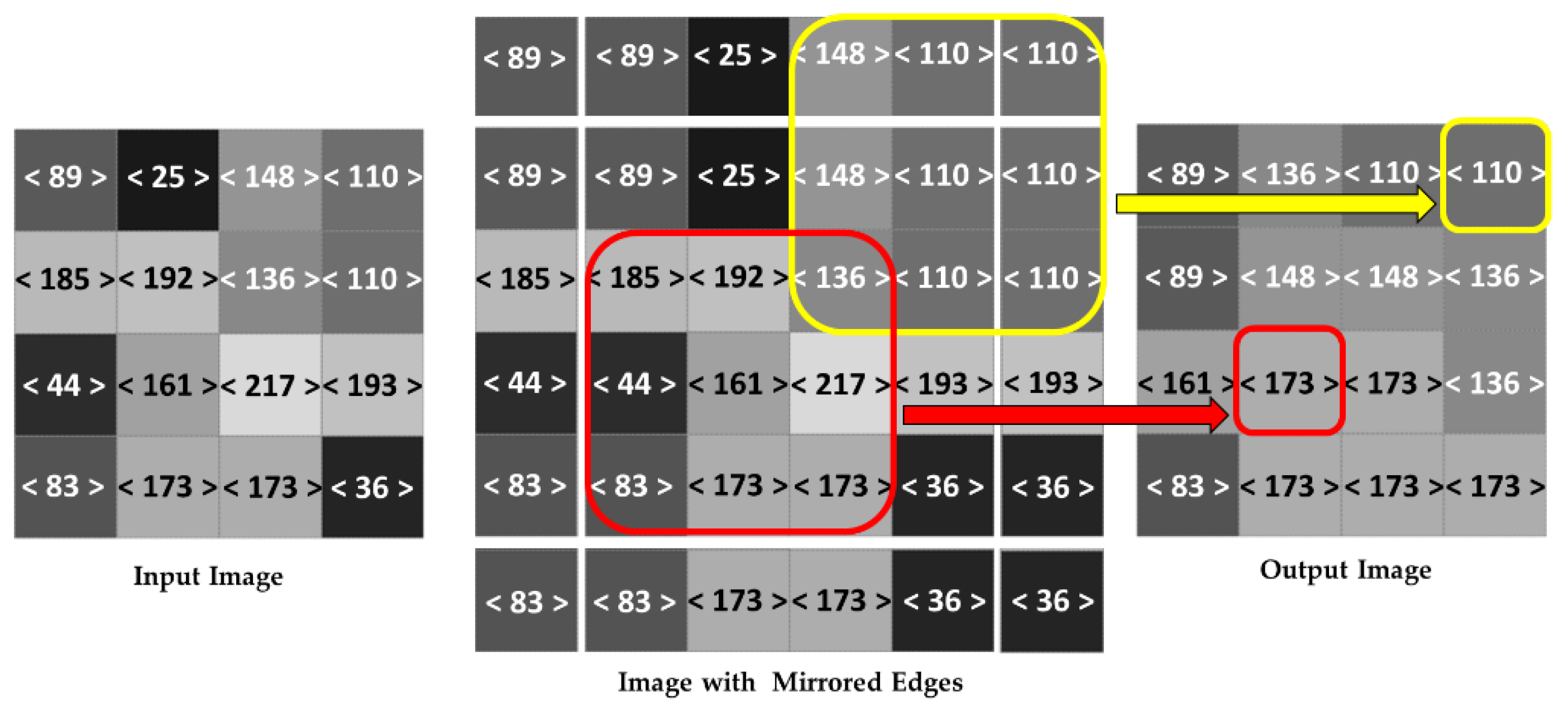
The median filter performs the image data smoothing by removing the noise from images. It operates as a sliding window to improve the results in later processing, leaving the image cleaner, which calculates the median value on the neighborhood from the specific pixel considered, removing the impulsive noise and preserving the edge border, which is important for detecting objects in the image. In image processing, the median filter replaces the central pixel with the median of the neighboring area pixels. Thus, it is an efficient method for noise reduction of individual peaks coming from the environment where the noise could lead to high contrasts in the image, which would be propagated to the binarization stage [23].
Figure 7 illustrates the process of median filter application in the image at the pixel level. First, there is a specific set of pixels with their respective intensity as an input image. The image is then analyzed pixel by pixel, with the mirrored edges along the border of the initial image, to solve the problem of executing a neighborhood operation in a border pixel. Finally, the average value of each pixel is determined, and a new image is generated as an output image, as depicted by the yellow and red marks.

Figure 7.
The median filter in the intensity image.
The neighborhood averaging can suppress isolated out-of-range noise for this method, but the side effect also blurs sudden changes, such as line features, sharp edges, and other image details corresponding to high spatial frequencies.
This way, a median filter is an effective method that, to some extent, can distinguish out-of-range isolated noise from legitimate image features, such as edges and lines. Specifically, the median filter replaces a pixel by the median, instead of the average, of all pixels in a neighborhood . Equation (2) details the application of the median filter, where represents a neighborhood defined by the user, centered around image location [24].
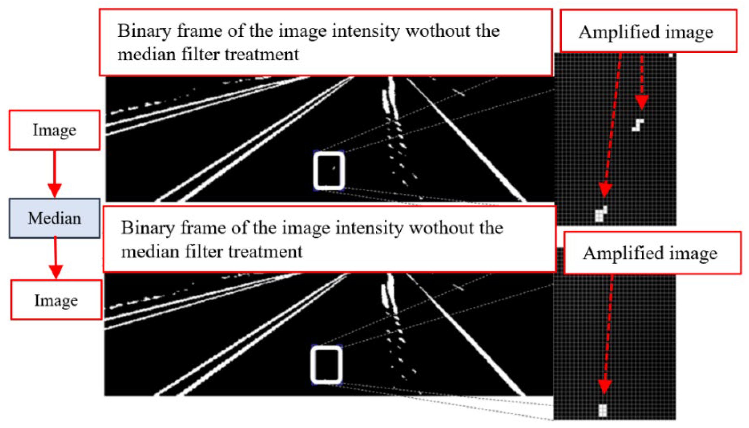
The median filter has noise an attenuation efficiency that can generate random points in the binarization step. For example, Figure 8 shows a case study in which noise is identified, such as ‘1’ binary points, and when applying the median filter in the intensity image, 1-bit binarization of that noise is avoided. Therefore, the definition of the filter neighborhood must satisfy the need for attenuation of possible noises in the image.
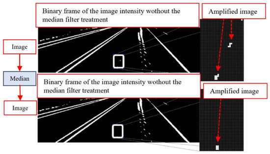
Figure 8.
Attenuation of noises with a median filter applied in the intensity image.
Figure 8 shows that the image is already in a specific ROI containing the recognized objects. The image still has some small undesirable noises, but that does not affect the main objects of interest.
Although we have already treated the frame in several aspects to obtain a clean and good quality image, it can still have some characteristics of blur or noise. Then, the most common technique adopted to remove these undesirable situations is a Gaussian smoothing operator [25,26], a 2D convolution operator.
3.3. Two Dimension (2D) Gaussian Filter
While the median filter removes the impulsive noises, the Gaussian filter aims to make the blurry image sharper. The mathematical operation for the image in 2D space is carried out by Equation (4). In practice, when computing a discrete approximation of the Gaussian function for pixels in the image at a distance of more than 3σ, there is a small enough influence to be considered effectively zero. Then, we used the image-processing algorithms to calculate a matrix with dimension 6σ per 6σ to guarantee that we are not losing information.
The Gaussian smoothing operator is a 2D convolution operator used to ‘blur’ images and remove detail and noise. In this sense, it is similar to the mean filter, but it uses a different kernel that represents the shape of a Gaussian (‘bell-shaped’) hump.
The Gaussian distribution in 1D has the form shown in Equation (3), where σ is the distribution standard deviation. We have also assumed that the distribution has a null mean (centered at the line x = 0).
In 2D, the isotropic (i.e., circularly symmetric) Gaussian distribution has the form described in Equation (4).
The main idea of Gaussian smoothing is to use this 2D distribution as a point-spread function that is achieved by convolution. Thus, from the image stored as a collection of discrete pixels, we need to produce a discrete approximation to the Gaussian function before performing the convolution. In theory, the Gaussian distribution is non-zero everywhere, requiring an infinitely large convolution kernel, but in practice, it is effectively zero, more than three standard deviations from the mean, so that we can truncate the kernel at this point.
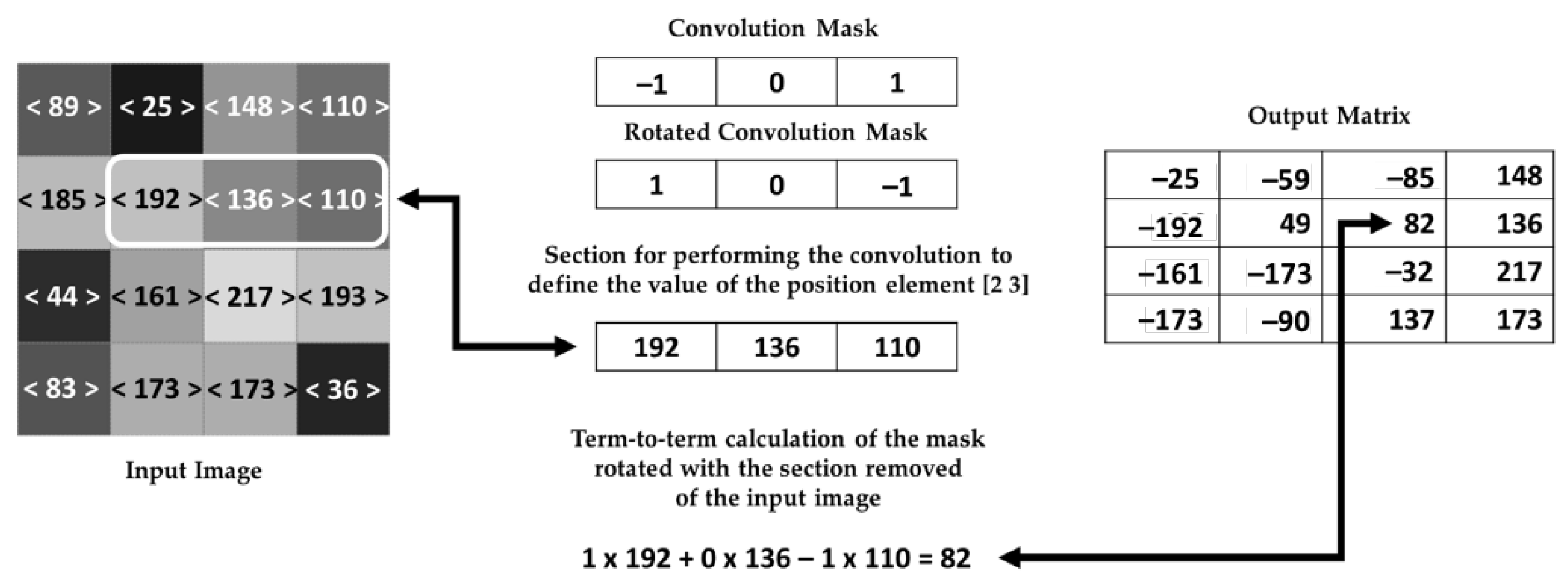
Then, the 2D Gaussian filter consists of a convolution with a particular mask applied to the pixels of the image and is an efficient form to suppress Gaussian noises [27,28] that originate from lighting situations in the transmission and image capture processes. This operation is performed in every pixel of the image, as shown in Figure 9.
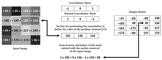
Figure 9.
The 2D Gaussian filter using the convolution process.
Firstly, the mask elements are inverted, and the inverted terms are multiplied with the corresponding terms of the addressed matrix. Then, the result is allocated in the output matrix element that corresponds to the central location of the mask element. After making the operation in an element, the process restarts in other positions of the addressed matrix. Finally, the elements at the edge of the input image and the convolution mask elements outside the image dimensions are multiplied by zero with no contribution to the pixel output value.
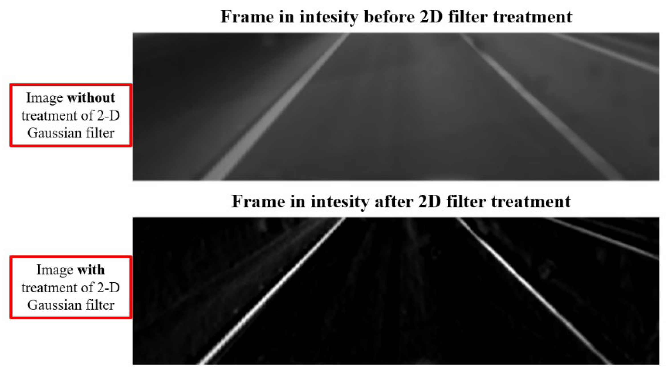
The 2D Gaussian filter has a noise attenuation property, which can directly influence the image resulting from the binarization process, or it can also be used to amplify and attenuate specific values in the intensity image. For example, Figure 10 shows the process of high-value pixel amplification (bright pixels) and attenuation of low-value pixels (dark pixels) of the grayscale image. Therefore, the mask definition for convolution must satisfy the robustness of the system considering the range of values of the pixels to be attenuated and/or amplified.
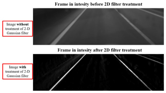
Figure 10.
Attenuation and amplification of ranges with values by the 2D Gaussian filter.
After applying the 2D Gaussian filter, the image can go through the thresholding process or transform a grayscale image to a binary one [23]. In this case, Otsu’s method is applied to the filtered image.
3.4. Otsu’s Method
In computer vision, Otsu’s method is deployed to perform clustering-based image thresholding automatically. It is assumed that the image contains two classes of pixels following a bi-modal histogram (foreground and background pixels). The algorithm calculates the optimum threshold separating the two classes so that their combined spread (intra-class variance) is minimal or equivalently (because the sum of pairwise squared distances is constant) so that their inter-class variance is the maximal one [25].
The binarization of the image in intensity is performed through Otsu’s method. The method consists of analyzing the histogram with the extraction of weights, means, and variances to decide the intensity threshold for the binarization.
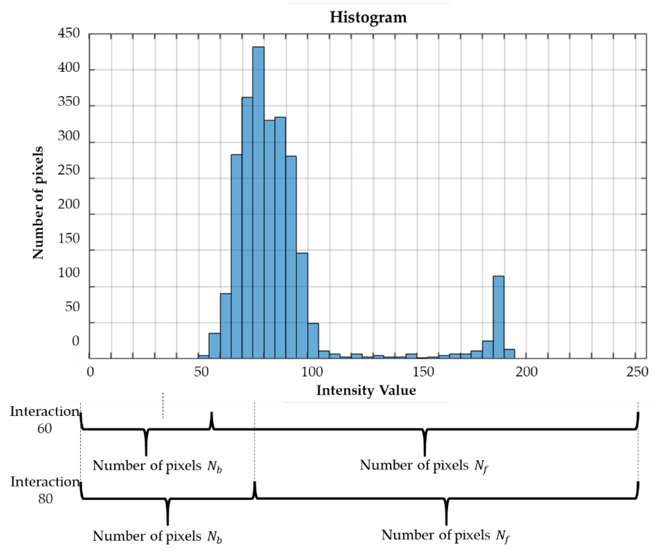
The process begins with the histogram building and division into two groups of pixels, foreground and background. At each code interaction, the sizes of the foreground () and background () pixel groups are modified, as shown in Figure 11. The intensity of the background group in the interaction is the binarization threshold that is computed.

Figure 11.
Definition of and through a histogram.
The size of the background group starts with the smallest value of the histogram and grows to the maximum value, and the size of the foreground group is complementary to the value of the background group, as shown in Figure 11.
After defining the number of pixels and their respective values in each group ( and ), the calculation for the definition of weights, Equations (5) and (6), and are performed.
With the weights defined, the calculations are performed to define the mean values of the groups, Equations (7) and (8), and using the pixel intensity values ( and ). Since and are the quantities of pixels with their respective intensity values and .
After the definition of the average values, the variance of values of the groups, Equations (6) and (7), and are calculated using the mean values obtained in Equations (9) and (10).
The definition of the joint variance of the groups, Equation (11), is the sum of the variances of the groups multiplied by their respective weights.
In the sequence, the other interactions are performed for all values of the background group. Then, the interaction with the lowest value of joint variance is chosen. Finally, the binarization threshold is defined as the intensity value for the position of the value of the size of the background group.
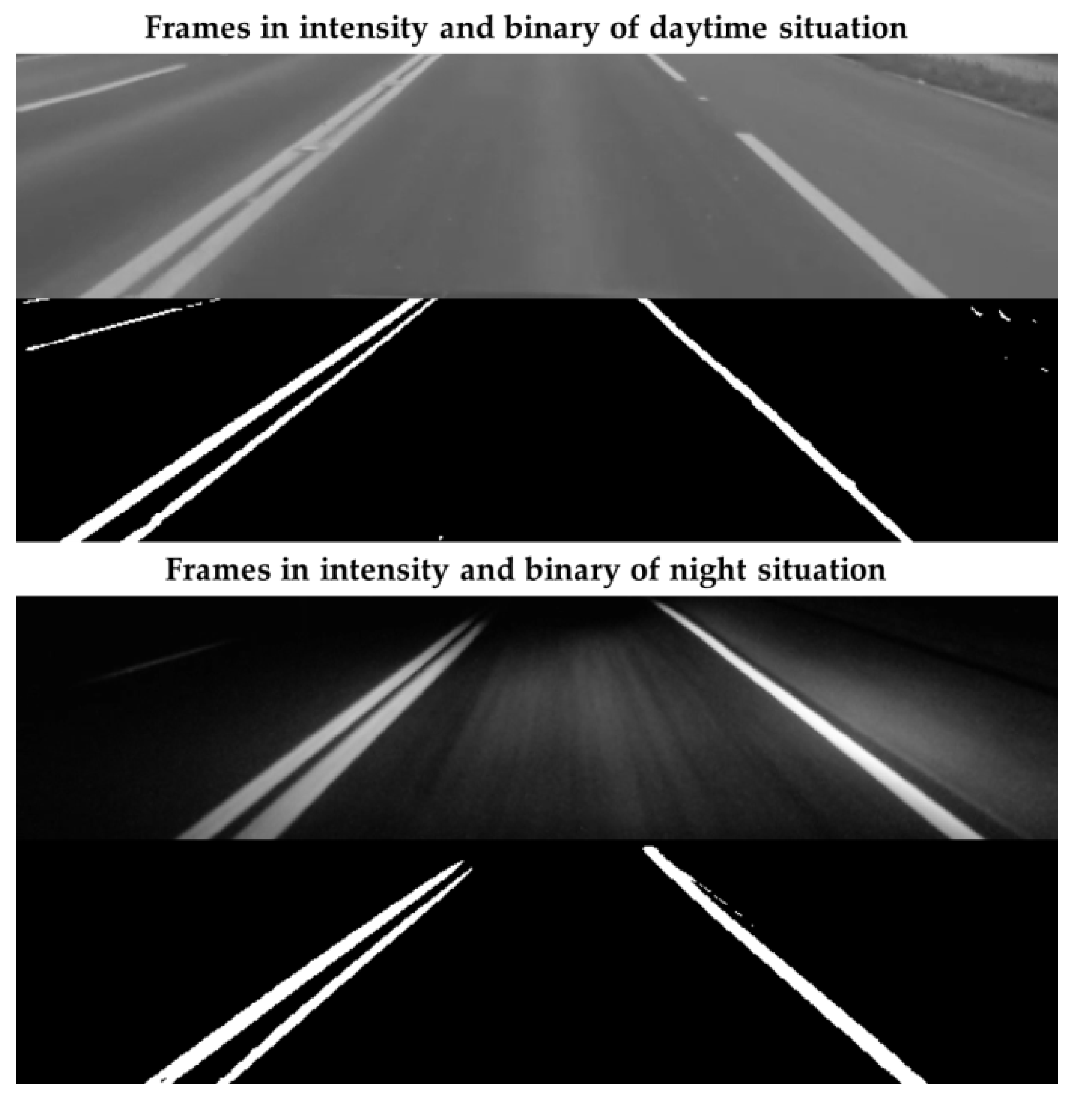
The lowest value of joint variance for the histogram image of Figure 9 was 333.12, characterizing the background group size of 2368 pixels. With this size of the background group, we have the intensity value 128, so this is the value of the threshold for binarization. Then, all pixels with intensity values more significant than the defined threshold are binarized in pixel ‘1’ and the others in pixel ‘0’. Thus, Otsu’s thresholding method guarantees the robust binarization of noise in different situations due to its analysis of variances for binarized groups. Figure 12 shows two cases with different illuminations in which this process of binarization ensured sufficient extraction of information from the intensity image.
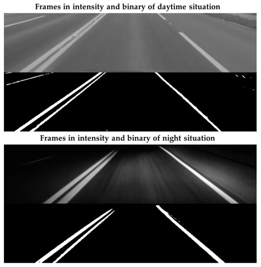
Figure 12.
The process of binarization in day and night situations.
3.5. Binarized Buffer
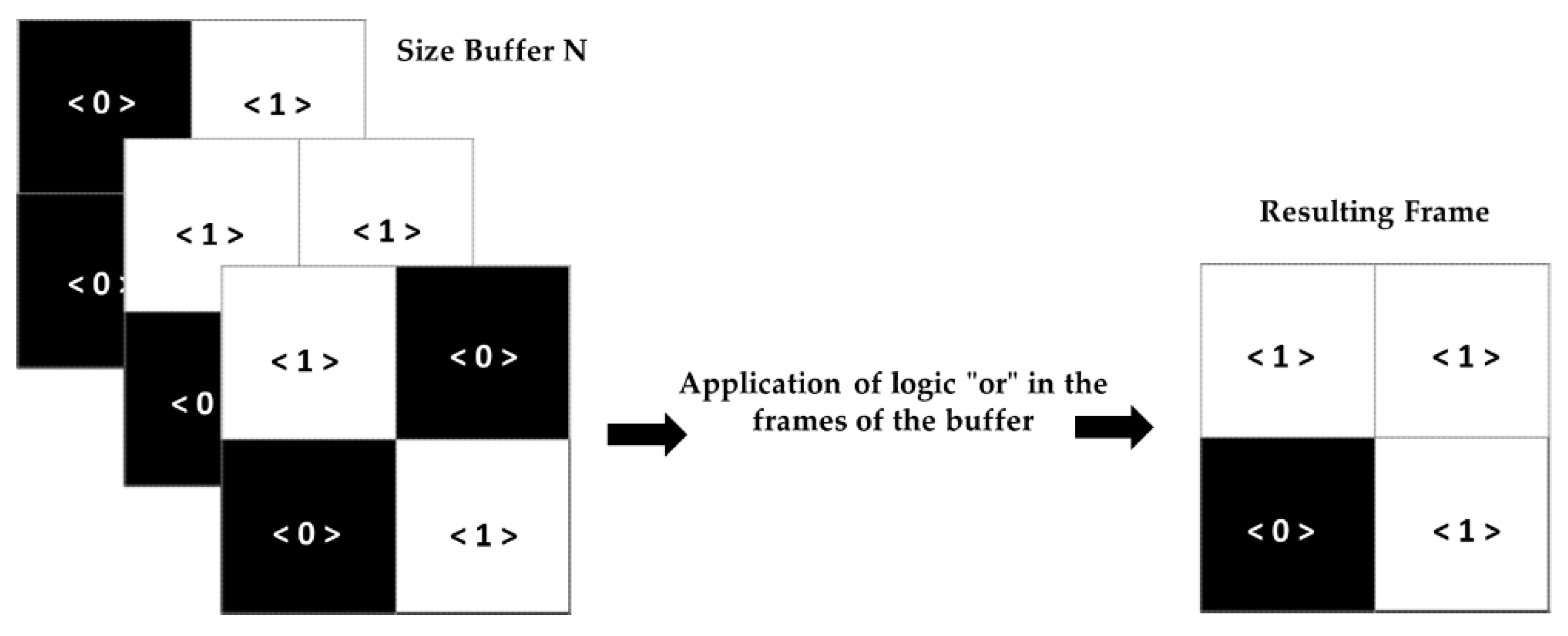
Binary buffering (Figure 13) consists of storing the binary frames according to the defined buffer size. The output frame is the execution of “or” operations on the buffer frames, i.e., whether a pixel is ‘1’ in any of the buffer frames, the pixel in the resulting frame is ‘1’.

Figure 13.
The process of binary buffering.
This process of binary buffering has efficiency in the possible intervals of lack of information in the lane marking, that is, at times when the frame has binary banding behavior, and in a near interval, there is no such behavior, a situation widespread in dashed lane markings. Therefore, as depicted in Figure 14, this buffer was applied to avoid information losses in this scenario and error occurrences for the next steps of the algorithm. Therefore, the size of the binary buffer must satisfy the lack of information in moments when the camera captured ROI is between two-lane marking segments.
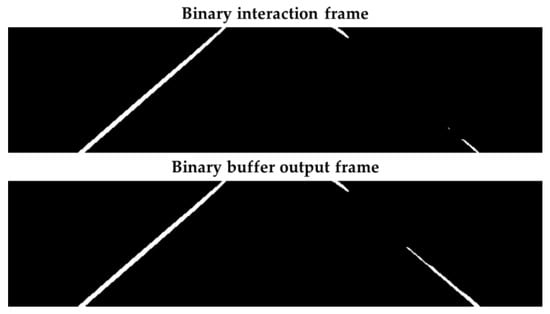
Figure 14.
The process of binary buffering in the segmented band.
4. Processing
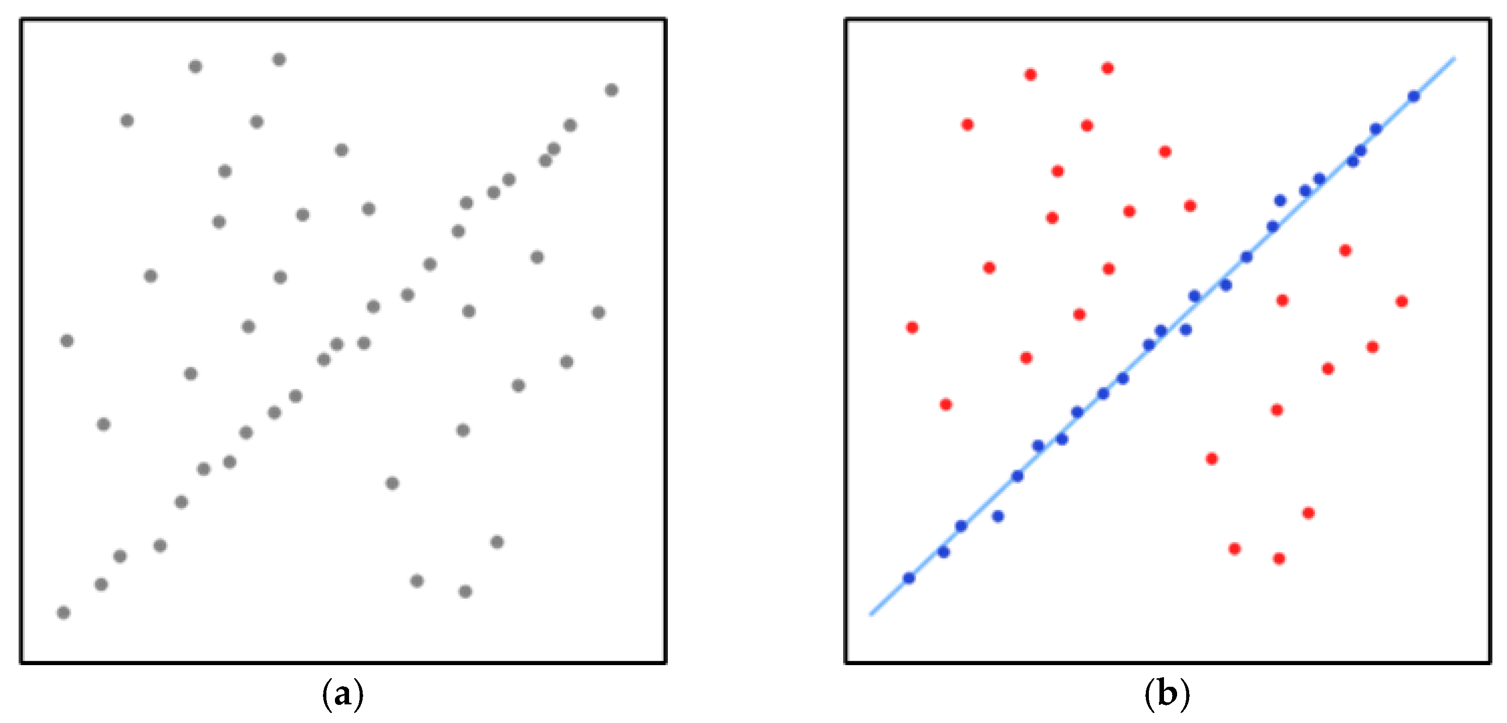
RANSAC [26] is an iterative method to estimate the parameters of a mathematical model from a set of observed data. Therefore, it also can be interpreted as an outlier detection method. Furthermore, it is a non-deterministic algorithm because it produces a good result only with a certain probability, with this probability increasing as more iterations are allowed.
A simple example is the fitting of a line in two dimensions to a set of observations. If this set contains both inliers, i.e., points that can be approximately fitted to a line, and outliers, points that cannot be fitted to this line, a simple least-square method for line fitting generally produces a line with a bad fit the inliers. The reason is that it is optimally fitted to all points, including the outliers. On the other hand, RANSAC can produce a model that is only computed from the inliers, provided that the probability of choosing only inliers in the selection of data is sufficiently high.
Figure 15 shows the application of the RANSAC method that aims to recognize the fitted line. Figure 15a shows the data set with many outliers, and Figure 15b shows the fitted line in blue through the RANSAC method so that it is possible to recognize the road lane at the image frame. Therefore, the RANSAC is the simplest method to recognize road lanes even in curvature because it can be segmented into small pieces having an almost straight line with good accuracy and precision. Moreover, it requires fewer computer resources than advanced algorithms to carry out the recognition process. The critical point is that the road lane can be straight or curved, which leads to applying, respectively, Linear RANSAC or Parabolic RANSAC.
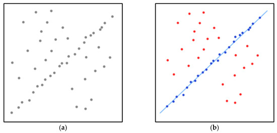
Figure 15.
(a) A data set with many outliers for which a line has to be fitted. (b) Fitted line with RANSAC; outliers do not influence the result.
4.1. RANSAC Method to Road Lane Recognition
After the development of the RANSAC code, several strands have been developed. All RANSAC codes contain two main bases, the hypothesis and the test. The hypothesis stage consists of the model’s definition that is sought using the minimum sufficient quantity of the input sample to obtain such a model. Concerning the RANSAC code in this investigation, we used parabolic and linear models, which require at least three and two samples of the input group, respectively.
After the sample selection, the coefficients of the characteristic equation are extracted by the inverse matrix method as shown for the parabolic model in Equation (12).
Then, the X-axis values of all points ’1’ are used to find the corresponding Y-values through the coefficients of the equation found () and then the real Y-values () are compared with the values found. Figure 16 exemplifies the divergence of the model found in the interaction with the entire sample group.
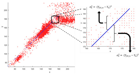
Figure 16.
Calculation of the quadratic error for all analyzed points.
Subsequently, the quadratic error values of each element are compared with a threshold for classification between inliers (belonging to the sought-after model) or outliers (not belonging to the sought-after model). At the end of an interaction of the algorithm, we have values of the coefficients of the model to be searched along with the number of inlier and outlier points. The interaction that obtains the coefficients with more inlier points is allocated as a response [27].
The number of interactions of the code is defined by Equation (13), which takes into account the probability that a point is not in the desired model (e), the number of points in a sample (s), and the desired probability in a representative interaction (p), that is, an interaction that represents the model sought through the coefficients found. Therefore, the value p is set to 0.99, stipulating that the chosen random points are not out of the sought pattern in at least one interaction.
However, to use Equation (12), the number of outlier points must be known, which impaired their application in this work because this number of points is variable for each frame analyzed. Therefore, we used Equation (14), which is calculated in the whole interaction as limiting the number of total interactions of the algorithm. In this equation, the coefficient ε is used, representing the probability of not selecting minimum samples representing the searched model, labeled as a false alarm rate. Additionally, the coefficient q that approximately represents the probability of selection by k (degree of the sought model) times of point inliers of the total of points is used. The coefficient q can be obtained through Equation (15), which considers the number of inliers of the interaction () and the total number of analyzed points ().
If the current interaction is greater than the coefficient , the code is interrupted, and the interaction coefficients with the most significant number of inlier points are sent as the final response. There are some control parameters of interactions that are not dependent on the intrinsic probabilities of the analyzed points, although they are dependent on the time and processing expenditure that the code can achieve, such as the maximum number of interactions, the maximum number of interactions without the improvement of the index of inliers points and the minimum of interactions that the algorithm should perform. In hierarchical order of variables, first, the minimum of interactions is carried out, and later the code can be interrupted by the other parameters.
4.2. Processing Step Development
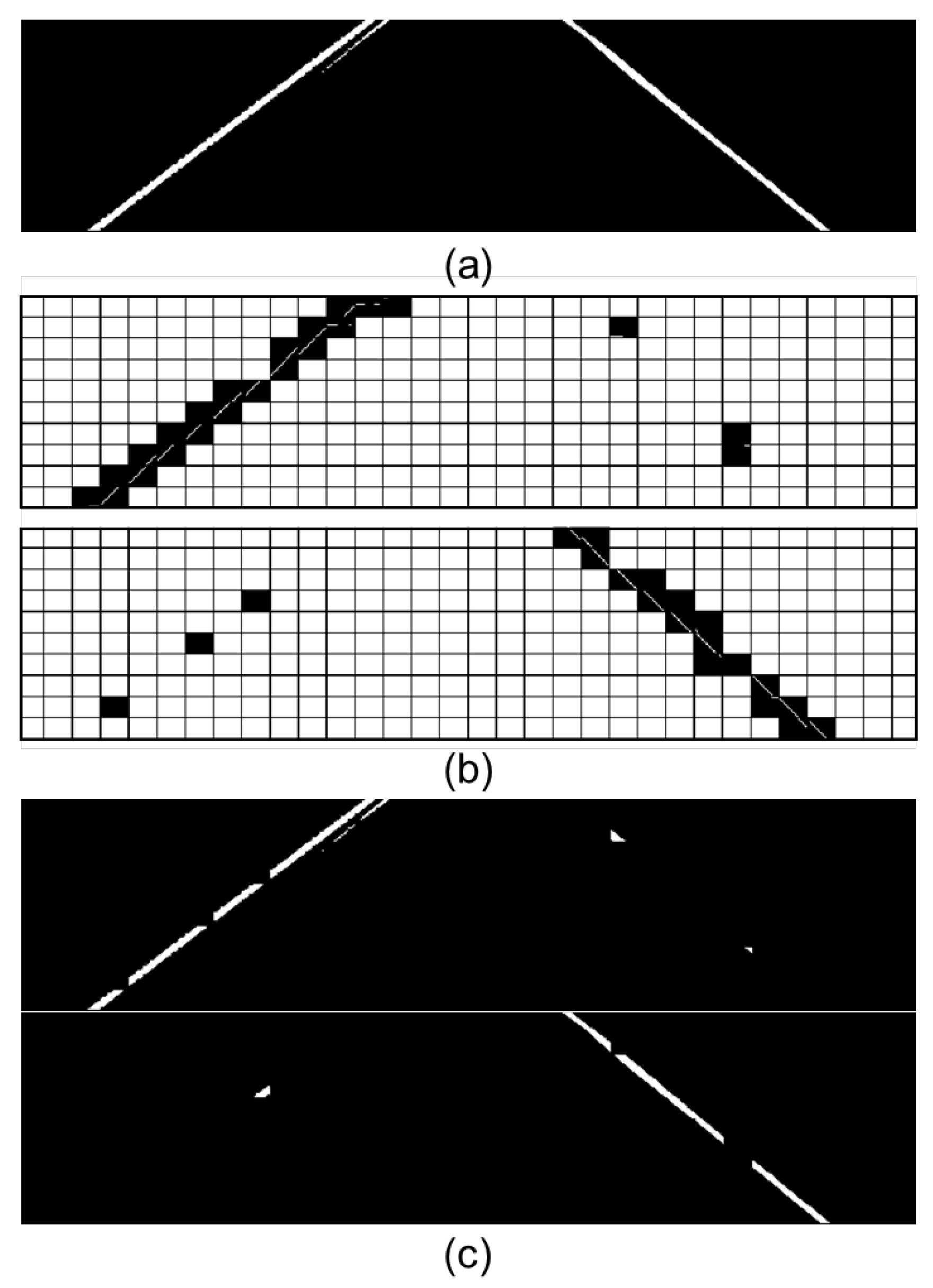
This step begins with subdividing the binarized image from previous processes into smaller quadrants for the best fit and identification. Next, the linear model of the RANSAC method is applied in each of the sections, and with the identification of the pattern, the spatial arrangement of the lane markings is identified by the angular coefficient analysis (Figure 17). If the coefficient is positive, the section is related to the left lane marking; if it is negative, it is related to the right-side lane marking. The linear model’s application in a section must contain a minimum number of white pixels, and if not, this section is discarded. Finally, if the section is valid, the area of the corresponding section of the binarized input image is allocated in separate images according to their respective values of the angular coefficients.
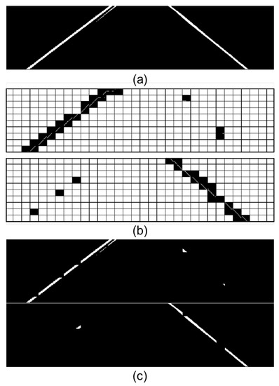
Figure 17.
Application of the RANSAC linear model in the subdivisions of the binarized image. (a) Input image; (b) application of the RANSAC linear model in the subdivisions of the image; (c) corresponding sections of the input image to sections with valid linear models. The upper image corresponds to the sections with positive angular coefficients and the lower ones with negative angular coefficients.
At the end of this step, two binarized images represent patterns to the left and right of the image. Next, the pattern recognition algorithm is applied in a parabolic model to match the identified sections with these images. As a result, the coefficients of the parabolic model representing the lane markings are extracted. Figure 18 shows the pattern found by the parabolic algorithm.
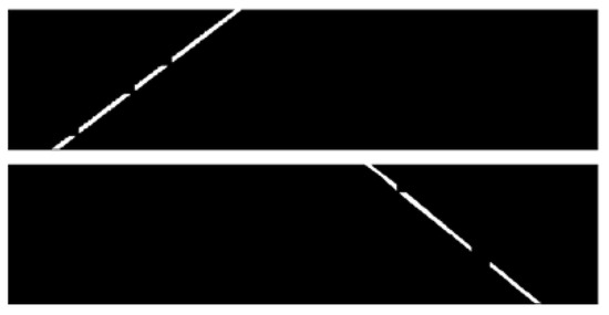
Figure 18.
Application of the parabolic RANSAC model. Corresponding points of the input image to the parabolic RANSAC equation found for the left and right bands, respectively, for the track model employed: .
After that, the interactions of the RANSAC code and the identified track model coefficients are made available to the following stage.
5. Post-Processing
The post-processing step verifies the integrity of the lane markings identified in the processing step with the extraction of points for the user’s visualization and alerts in case of a runway exit.
5.1. Integrity Verification of Road Lane Marking
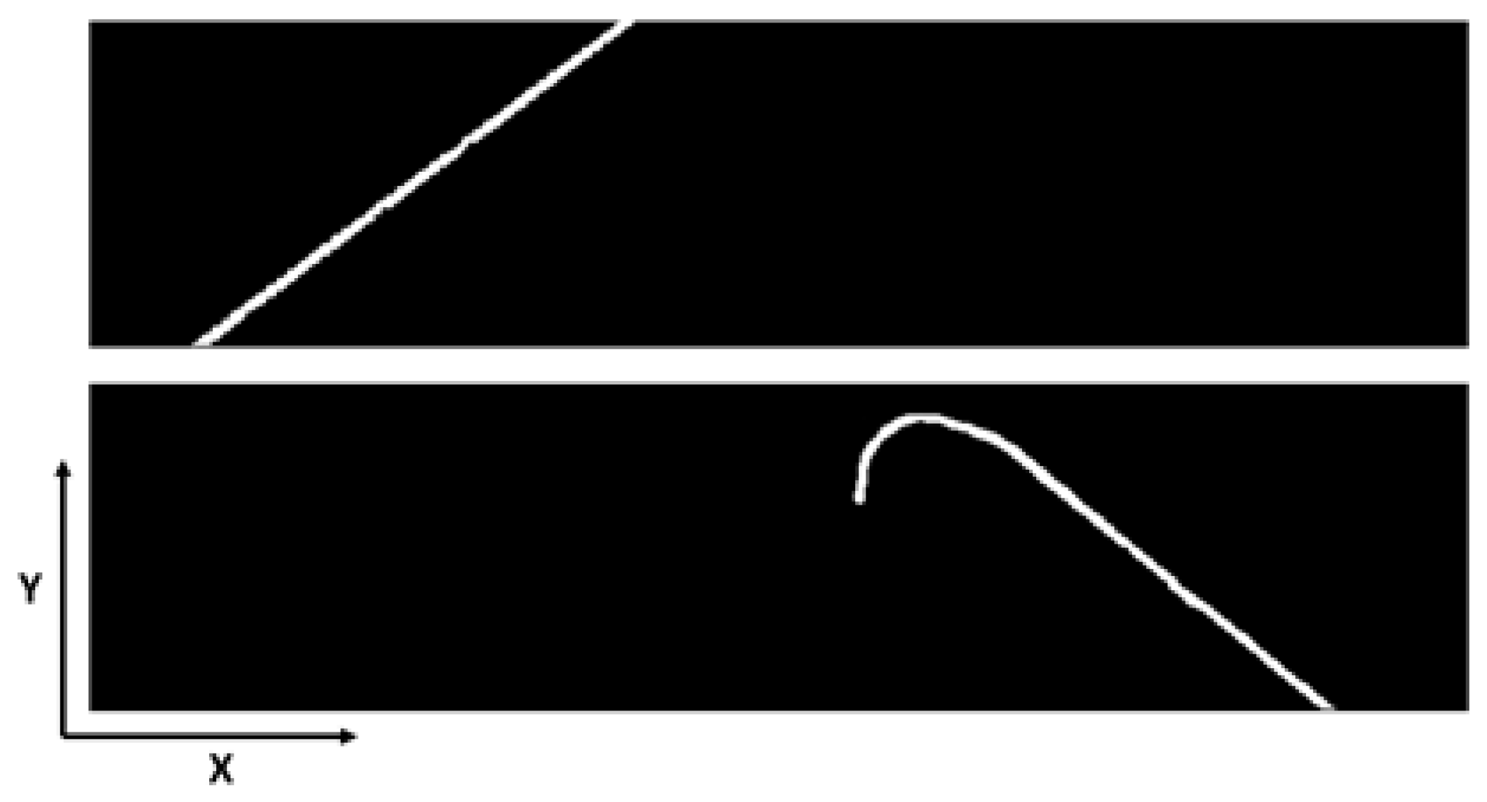
The integrity road lane marking verification step is performed through point repetition analysis or if they represent inconsistent lane marking models, as shown in Figure 19. Identifying these models is crucial for avoiding errors in distance calculations and maintaining point tracking for the next system interaction. There is also the identification of the coefficient value extrapolation, which may denote inconsistent models. As is the case of the module of the higher-order coefficient, if it is too high, it denotes an inconsistent lane marking model.

Figure 19.
Valid and invalid lane marking. Upper image: proper lane marking, without repetition of Y points and the coefficient “a” module within the calibrated range. Bottom image: Invalid lane marking, with repetition for Y points and the coefficient “a” module outside the calibrated range.
5.2. External and Internal Filters
External and internal filters track the current frame range according to the region close to the lane marking identified in past interactions. Therefore, the activation of these filters only occurs if there are valid coordinates of the tracks in past interactions. In that situation, the image filtering from the pre-processing is performed, and then it is forwarded to the processing step. On the other hand, there is no stage filtering from the pre-processing when there are no valid coordinates. Instead, this is sent directly to the processing step, as shown in Figure 20.
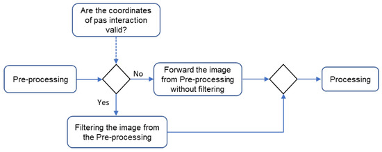
Figure 20.
Flowchart between pre-processing, processing, and post-processing.
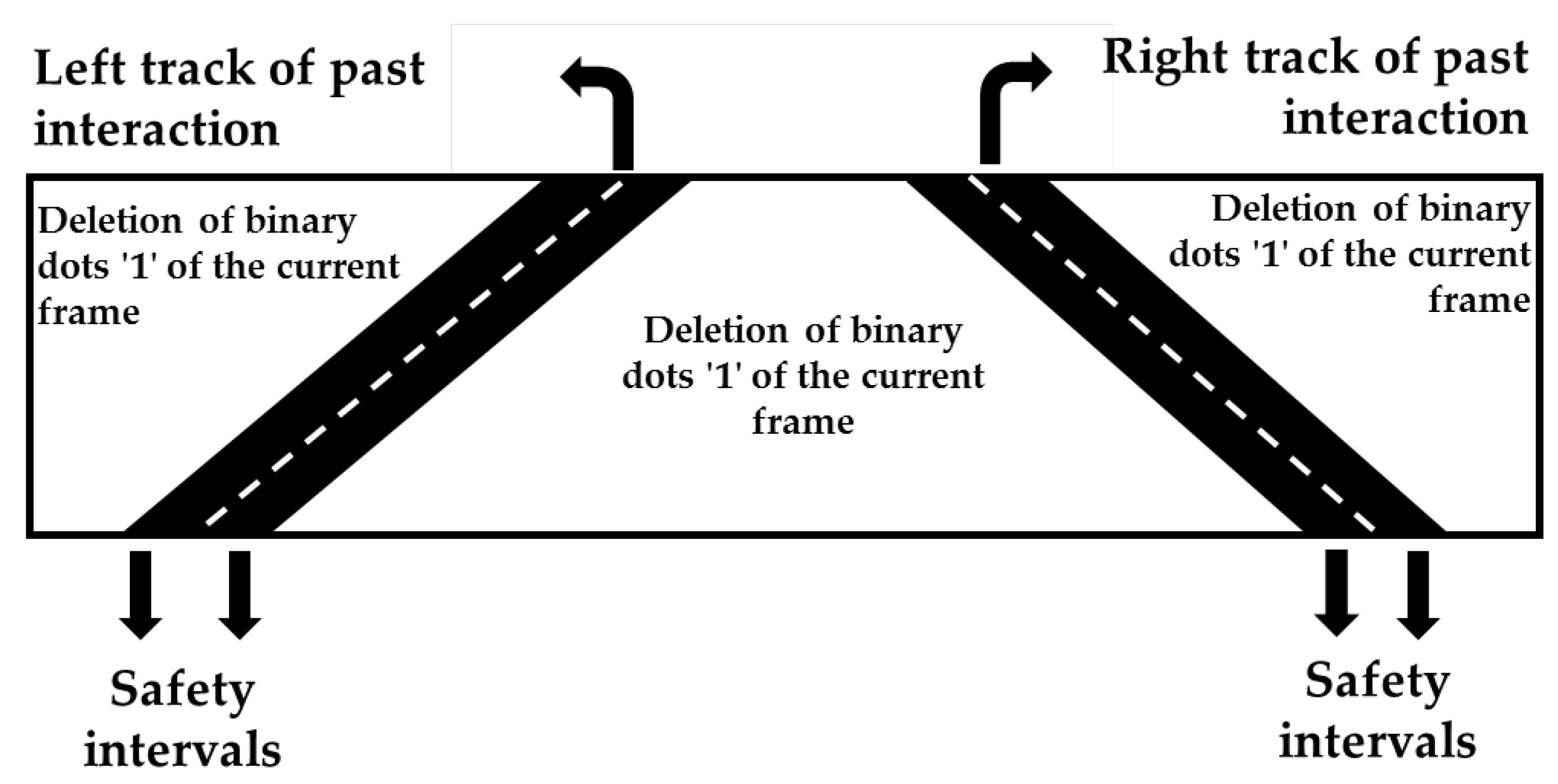
The filtering consists of deleting white pixel points from the frame of the current interaction against the past coordinates with a safety interval so that it does not compromise the integrity of the lane markings in the current frame, as depicted in Figure 21. The central area between the markings consists of the internal filtering, and the upper areas of the edges consist of external filtering.

Figure 21.
Internal and external filtering process.
The stages of pre-processing, processing, and post-processing could be deployed for the features that need to be recognized in this case. For example, the following section shows how it can be applied for LDW or LKA that relies upon road lane marking recognition to measure the vertical distance between them, and the medium value is the reference point that the vehicle center point should be kept.
After checking the integrity of the lane markings, the LDW is calculated to define whether the vehicle is evading its track. In this calculation, the field is considered near the image to obtain data (Figure 22).
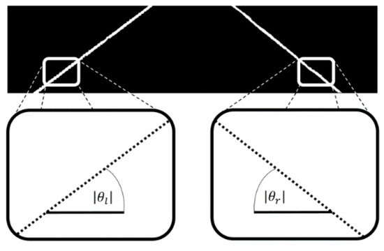
Figure 22.
Obtaining the angles of the tracks for the LDW calculation.
In the near field, the extraction of some samples of the location of the bands with the linear approximation for the definition of the angle is carried out. By defining the angle, it is possible to identify the range output with analysis of the magnitude of the values with pre-established limits and activate or deactivate the alert for the driver.
After defining the LDW state, the coordinates of the identified track model are extracted to the user view. This step is essential because it allows a preliminary subjective analysis of the developer, which can help identify the system’s gross flaws or even non-functionality. Therefore, the outcomes in Figure 23 are visual and one of the verification steps before the quantitative verification step. Furthermore, qualitative verification can save development time if errors are identified, given that quantitative verification has a more significant expenditure of development time.
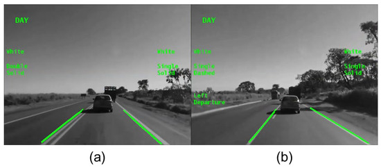
Figure 23.
(a) Visual algorithm output without LDW activation; (b) visual algorithm output with LDW activation in the left lane marking.
6. Case Study
For the tests, six cases composing over 4000 frames of the GSA database were used. The selected samples were taken at different climatic scenarios and road situations. In the climatic scenarios, some samples stand out due to the presence of rain, visual disturbance of the windshield, and visual disturbance of the water accumulated in the lane marking and samples in which there are no visual disturbances, that is, with less stress of the algorithm for the identification of the lane marking. Furthermore, the cases include daytime and nighttime situations, and there is diversification in road situations (double, single, continuous, segmented, yellow, and white lane markings).
The validation of the lane tracking strategy has been performed using the ground truth method, which consists of manual marking of the ideal lane marking the location (in this case, the inner edge of the lane markings) that are stored in an XML file, and then compared to those coordinates’ algorithm markings (besides that, there is a tool in Matlab® that already performs the ground truth). The comparison performed was based on the LPD (Lane Position Deviation) technique [28] and comprises a good indicator for evaluating the effectiveness of lane detection based on the metrics discussed here.
The algorithm used in this process has two primary interfaces. One for the ground truth was marking and the other for comparing the generated XML files [29,30]. There are the following steps for the marking process: selecting the sample, marking the ideal position of the tracks through clicks on the actual video, and storing these coordinates in an XML file. The storage of algorithm results is also performed by saving the coordinates of the identified tracks in a file with an XML extension [29,30].
Subsequently, the XML files are compared. The algorithm has two primary validations of the coordinates, by Precision by Line (PPL) and Precision by Frame (PPF). The PPL (Figure 24) consists of the line-by-line check of the ideal marking for the algorithm output [29,30].
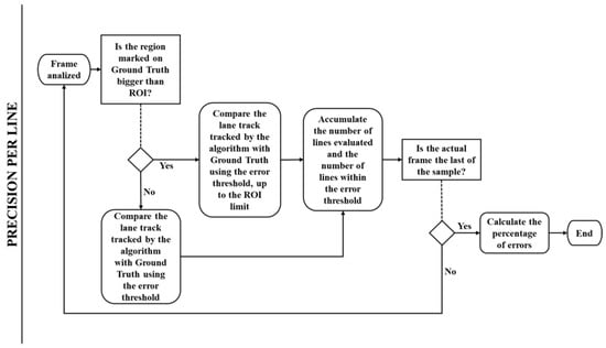
Figure 24.
Precision per line flowchart.
The PPF (Figure 25) consists of verifying a user-informed threshold with the Mean Absolute Deviation (MAD) of the optimal coordinates to the output coordinates of the algorithm. The algorithm still provides the Standard Deviation (SD) of the analyzed track markings.
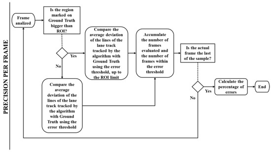
Figure 25.
Precision per frame flowchart.
After verifying the XML files, spreadsheets with CSV extension are generated for the interpretation of the data. With these worksheets, it is possible to obtain information on each sample and the general averages of the two verification processes. For each sample, the indices for the left and right bands were obtained with the ROI variation in 100, 120, 140, and 150 pixels (lines), and for each ROI value, the error threshold was varied in the values of 10, 15, and 20.
To generate graphics for analysis of the method, the average of the and is given by Equations (16) and (18). Consequently, we can build up the graphics automatically through functions and described in Equations (17) and (19).
From now on, we can deploy practical examples. This might be seen in the case studies from 1 to 6 thereafter.
6.1. Case-1: Sample with Rain, Windshield Disturbances, and Runway Water
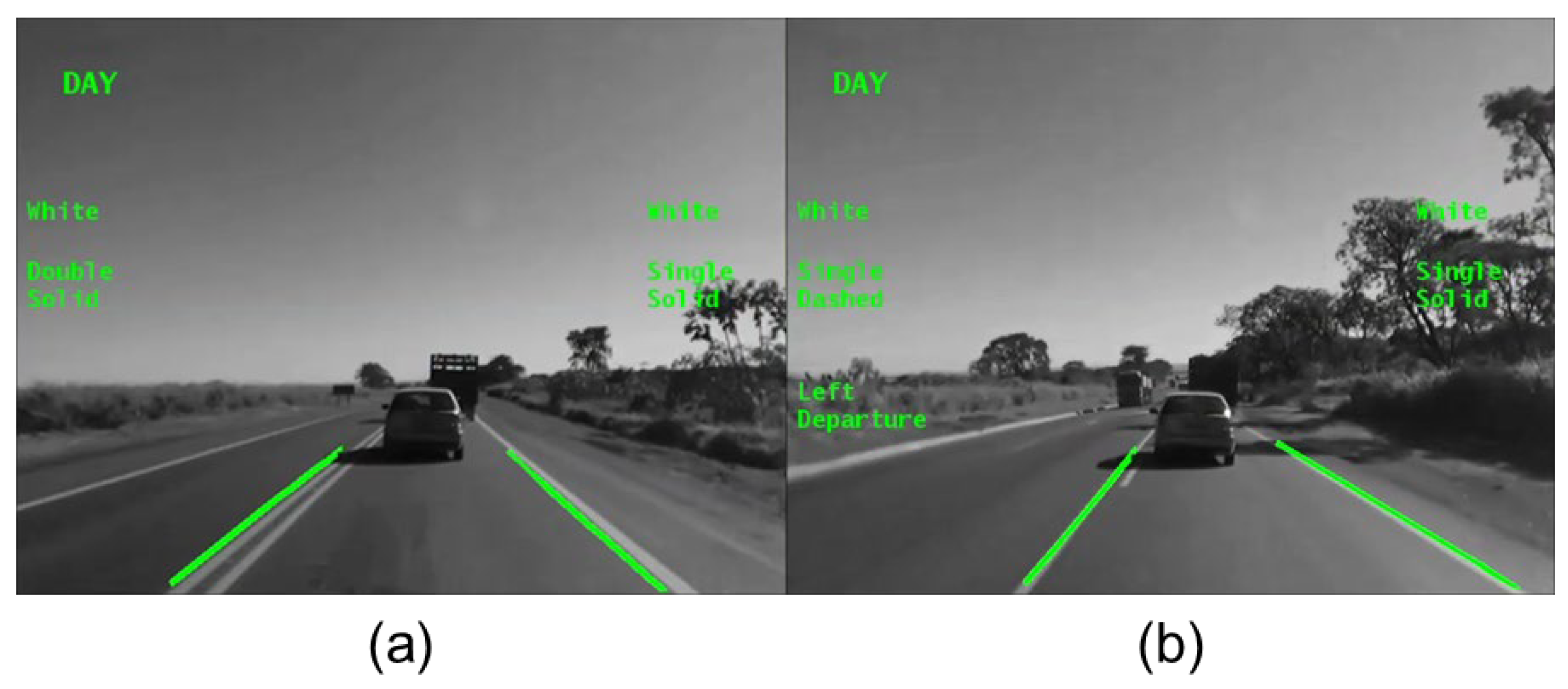
This sample contains 638 frames and elements that hamper extracting runway edges by the presence of windscreen, rain, and water noises in the runway, as shown in Figure 26a. In this case, the buffers played an essential role in keeping tracking stable even with the high stress of the algorithm and in a segmented band situation. The noise removal was appropriate for not compromising the identification of the tracks.
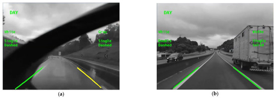
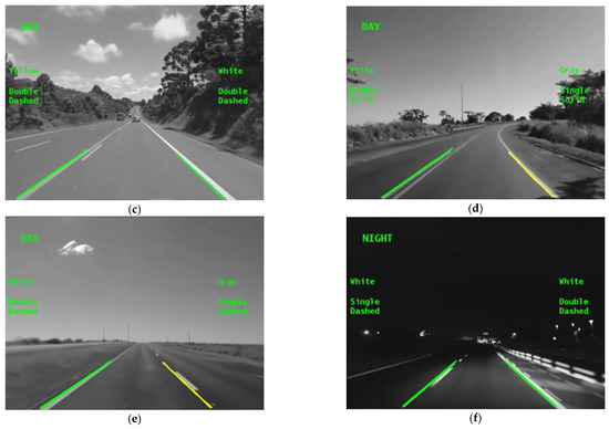
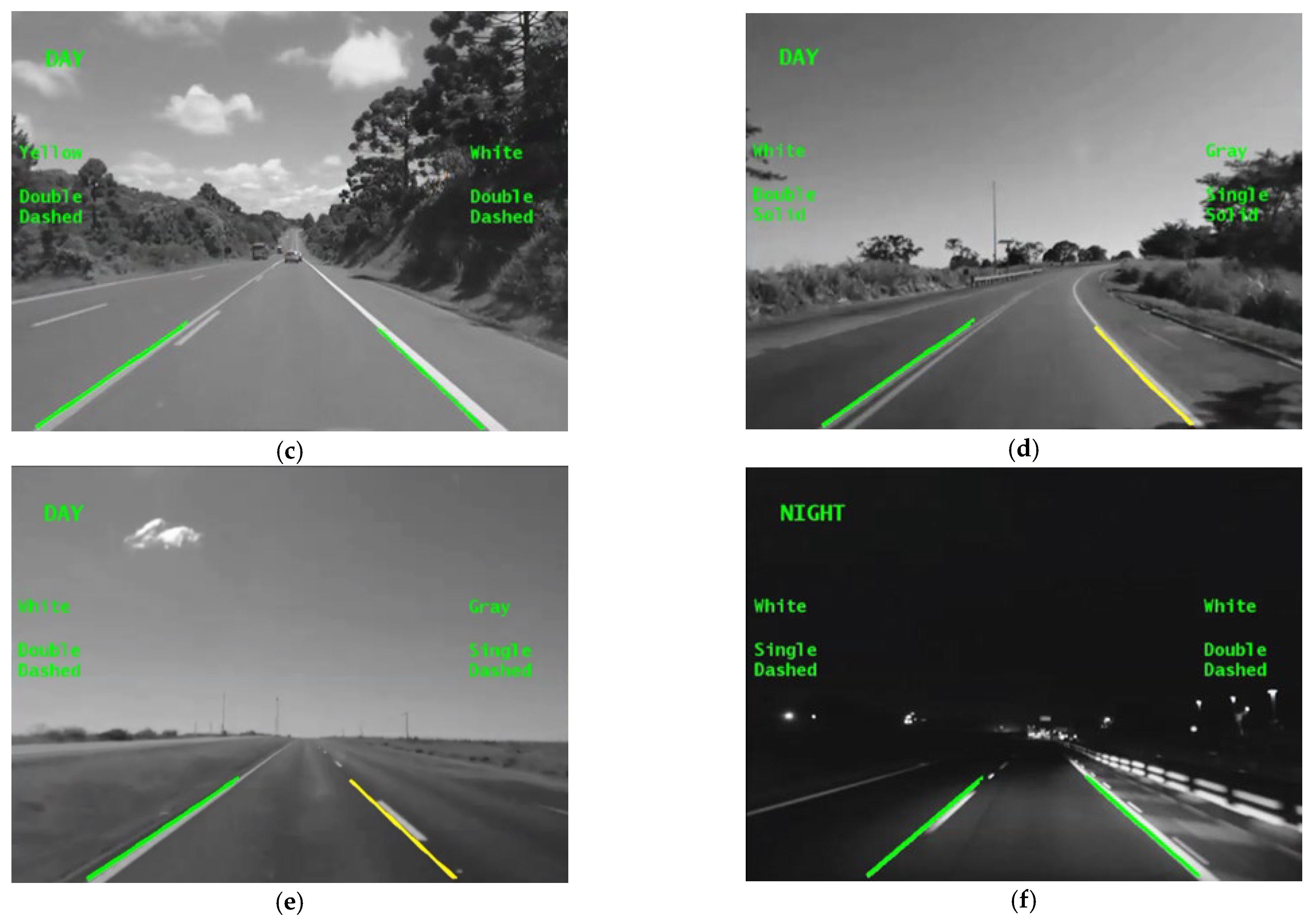
Figure 26.
Road images under different weather conditions, according to table I: (a) Case-1, (b) Case-2, (c) Case-3, (d) Case-4, (e) Case-5, and (f) Case-6.
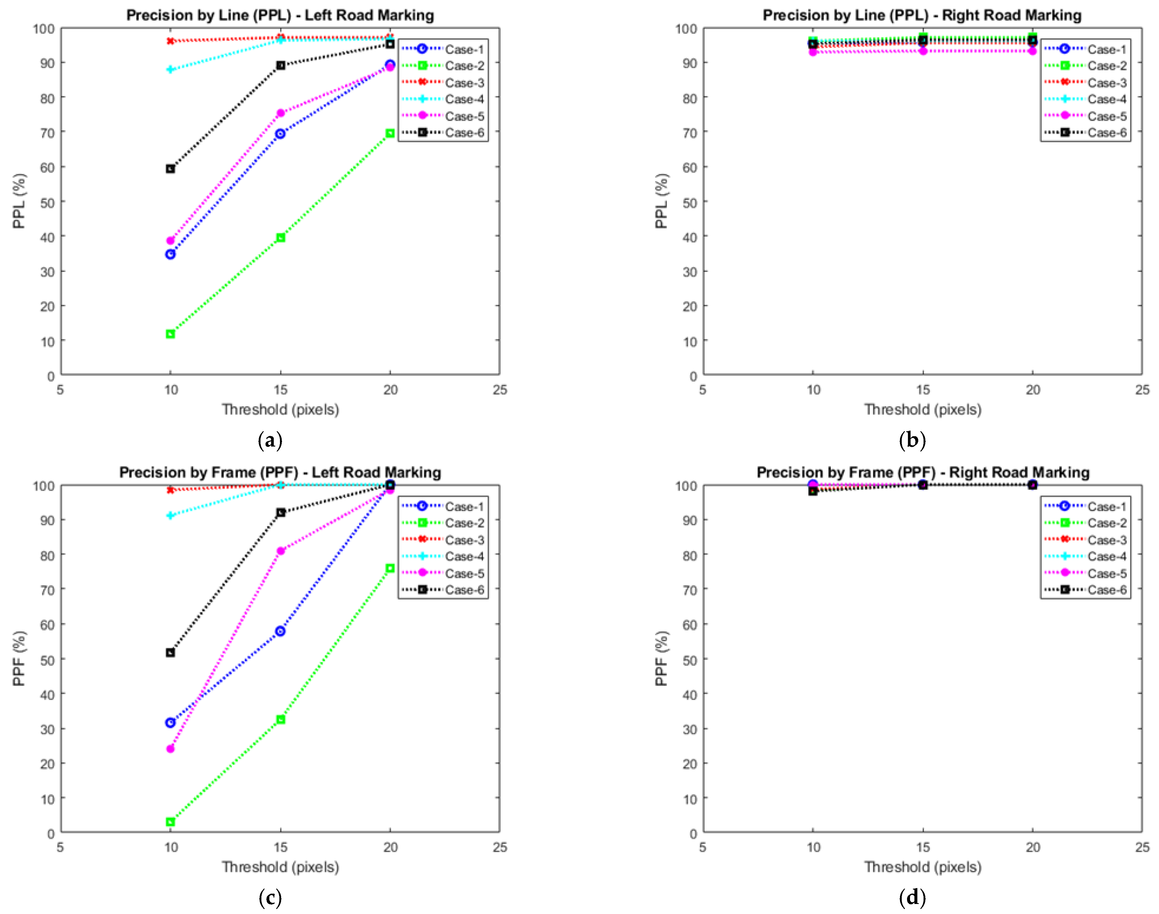
The analysis of the algorithm output for the left band is shown in Figure 27. It can be noticed that the increase in the error threshold directly influenced the result of the PPL and PPF, and there was a significant variation in the threshold indexes for all the ROIs. However, the modification of the ROIs had little influence on the PPL indices and none on the PPF indices. For all analyses, the MAD and SD remained stable with few variations.
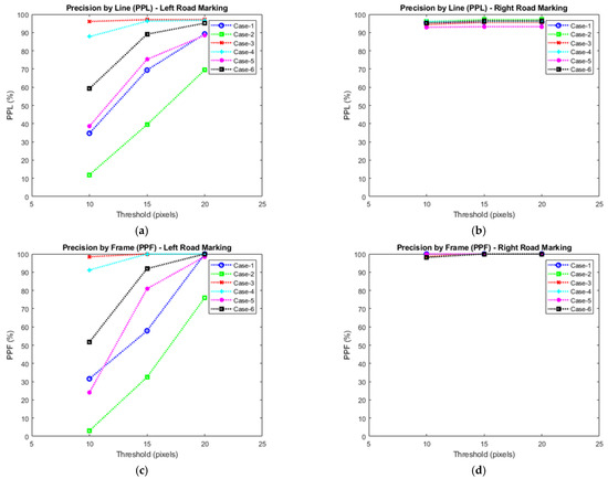
Figure 27.
Performance analysis by PPL and PPF: (a) PPL for road left lane marking, (b) PPF for road right lane marking, (c) PPL for road left lane marking, and (d) PPF for road right lane marking.
The error threshold increase influenced only the PPL result, and the PPF index remained stable in all the analyses. The change in ROIs had little influence on the indexes. For all analyses, the MAD and SD remained stable with few variations.
6.2. Case-2: The Band of the Left Was Continuous White, and the Right Band Was Continuous White, with a Small Segment Being Segmented
In this case, the sample is formed by 493 frames and contains no elements that are hampered to extracting edges of the track, as shown in Figure 26b. Therefore, identifying the bands was performed with less stress of the algorithm regarding identifying the bands in case-1.
The increase in the error threshold directly influenced the PPL and PPF results, and there was a significant variation in all the ROIs. For all analyses, the MAD and SD remained stable with few variations. The highest PPL and PPF values were 69.53% and 75.86%, respectively, even in a more favorable situation to identify the bands in this sample. This phenomenon is due to the ground truth metric marking the bands’ optimal coordinates as the inner edges. However, through the qualitative analysis, it was identified that the algorithm performed the recognition and marking of the outer border of the left band, compromising the quantitative indexes of PPL and PPF.
The increase in the error threshold influenced the PPF and PPL indices. The change in ROIs had little influence on the indexes. For all analyses, the MAD and SD remained stable with slight variations.
6.3. Case 3: The Left Lane Was Continuous, a Short Continuous Double, and at the End of the Double Segmented Video, Yellow throughout the Sample, and the Right Lane Was Continuous White
The sample is formed by 810 frames and contains no elements that are hampered to extract edges of the track or interference of noise from other vehicles, as shown in Figure 26c. Therefore, identifying the bands was performed with less stress of the algorithm regarding identifying the bands in case 2.
The increase in the error threshold directly influences the PPL and PPF, causing a significant variation in these indexes in all the ROIs. For all analyses, the MAD and SD remained stable with few variations. However, even in a more favorable situation for identifying the bands in this sample, the highest PPL and PPF values were 31.35% and 32.66%, respectively. The reason is that the ground thrush metric is used to mark the optimal coordinates of the bands to be the inner edges. However, through the qualitative analysis, it was identified that the algorithm performed the recognition and marking of the outer border of the left band, compromising the quantitative indexes of PPL and PPF.
The analysis of algorithm output for the right lane marking is shown in Figure 27 The increase in the error threshold had little influence on the PPF and PPL indices. Likewise, the change in ROIs had little influence on the indexes. For all analyses, the MAD and SD remained stable with few variations. In this case, the identification and marking of the bands were performed at the inner edge, and such behavior of the algorithm by the PPL and PPF indexes is explicitly high for all error threshold values.
6.4. Case-4: The Left Lane Was Continuous Double, a Short Stretch with a Simple Continuous Lane, Yellow throughout the Sample, and the Right Lane Was Continuous White
The sample is formed by 638 frames and contains no elements that are hampered to extract edges of the track or interference of noise from other vehicles, as shown in Figure 26d.
The increase in the error threshold directly influenced the results of PPL and PPF. The PPL index increased as the error threshold increased without much influence of the ROI variation, reaching lower and higher values, respectively, of 87.6% and 96.72%. In PPF, the most significant variation was increased the error threshold from 10 to 15 without influencing the ROI variations. For all analyses, the MAD and SD remained stable with few variations. Even in a more favorable situation for identifying the lane markings in this sample, the highest PPL and PPF values were 31.35% and 32.66%, respectively. Regarding this sample, the marking of the coordinates of the lane was performed according to the ground truth metrics. Furthermore, the values of PPF are rising with lower and higher values of 91.18% and 100%, respectively.
The increase in the error threshold and the ROI did not influence the PPF and PPL indices. The MAD and SD remained stable with few variations. In this case, the identification and marking of the bands were performed at the inner edge, and such behavior of the algorithm by the PPL and PPF indexes is explicitly high for all error threshold values.
6.5. Case-5: The Left Band Was Simple Continuous White, and the Right Band Was Simple Segmented White
The sample is formed by 377 frames and contains no elements that are hampered to extract edges of the track or interference of noise from other vehicles, as shown in Figure 26e. The increase in the error threshold directly influenced the results of PPL and PPF. The PPL index increased as the error threshold increased without much influence of the ROI variation, reaching lower and higher values, respectively, of 38.16% with an error threshold of 10 and 88.44% with an error threshold of 20. Analogous to PPL or PPF, a minimum value of 24.05% was obtained for error threshold 10 and a maximum of 98.53% for error threshold 20. For all analyses, the MAD and SD remained stable with few variations.
The increase in the error threshold and the ROI did not influence the PPF and PPL indices. For all analyses, the MAD and SD remained stable with few variations. The identification and marking of the bands were performed at the inner edge, and such behavior of the algorithm was explicit due to the high PPL and PPF indexes in all error threshold values.
6.6. Case-6: The Left Lane Marking Was Simple Segmented White, and Right Lane Marking Was Simple Continuous White at Night
The sample is formed by 667 frames, as shown in Figure 26f. The increase in the error threshold directly influenced the results of PPL and PPF. These indices increased as the error threshold increased without much influence from the ROI variation. The lowest and highest values were 58.95%, with an error threshold of 10 and 95.16%, with an error threshold of 20. The PPF obtained at least 51.70% values for an error threshold of 10 and a maximum of 100.00% for an error threshold of 20. For all analyses, the MAD and SD remained stable with few variations. The indexes with a threshold of error 10 verified that the left band’s external border was identified in some situations.
The increase in the error threshold and the ROI did not influence the PPF and PPL indices. For all analyses, the MAD and SD remained stable with few variations. In this case, the identification and marking of the bands were performed at the inner edge, and such behavior of the algorithm was explicit due to the high PPL and PPF indexes in all error threshold values.
6.7. Discussion
In this work, we proposed a thorough framework to support the algorithms to recognize objects from digital images. The object of interest in a road is the road lane used to keep vehicles in safe conduction and develop new features such as lane departure warning, lane-keeping assistance, and lane centering. The evaluation results show a significant performance gain of the RANSAC algorithm adopted with the buffering techniques. To assess the performance, we consider the performance index such as precision by line and precision by frame with the comparison between them.
Figure 26 shows the image frames from the road under different weather conditions, and Figure 27 shows the results generated from Equations (16)–(19), which allows assessing the performance to choose the best strategy to be adopted in an adaptive system. The frames that represent the digital images in frames are described in Table 1. We can see that the PPL and PPF methods for proper road marking have better accuracy and precision them road left marking, regardless of the threshold adopted. The better performance for the road right marking can be understood by taking into account the specificities of the Brazilian roads and the strategy used for ground truth marking. The GSA database was built with a majority of single-lane roads. The right side is the central line for single-lane roads, while the left side is the road’s shoulder. In single Brazilian roads, the central lane marks are usually present but with low quality, while the lane markings on the road’s shoulder are rarely identifiable. The strategy for ground truth marking ignored non-existent road marks so that the XML file generated to compare with the coordinates generated by the algorithm has fewer points to consider on the left side. Since the lane markings on the right side are of low quality, the XML file has more coordinates considered, and it is harder for the algorithm to calculate lines.

Table 1.
Description of the digital images in frames of case studies.
The results shown in Figure 27 confirm that the RANSAC algorithm behaved as expected. The high precision found on the results on the center lines shows the RANSAC capacity of delivering a robust estimation of a model even with a high level of outliners present in the data analyzed. Nevertheless, this may become imprecise when the system used does not have enough processing power. Since RANSAC needs several iterations to achieve higher precision, it may fail to find a model that fits the data set in a limited processing power environment. Another disadvantage of RANSAC is that a set of iterations estimates only one specific model. For DAS systems, the road lines and other desirable estimations always mix different models for straight lines, curves, and other road characteristics. In this environment, if RANSAC is used with a mixture of models within the same iterations, the calculation may fail for all situations, requiring additional iterations computed simultaneously to deliver the best suitable result for each model. The Hough transform is an alternative to variations of models inside the same calculation time. However, it does not have the same precision as RANSAC. Variations of RANSAC can also solve this downside by combining learning-based relevance scores. This workaround can rapidly change between different models to run the iterations without consuming too much computer power [31]. Another strategy already explored to improve RANSAC outputs is the use of guided sampling. Guided algorithms use available cues to assign prior probabilities of each datum, reducing the required number of iterations. However, it can make RANSAC slower due to the additional computation burden, which could impair the potential of a global search [32].
In the coming years, we are interested in expanding this work better to observe the performance of the proposed work with updated dissemination of intelligent algorithms that when merged can ensure a more robust system. Thus, it can also enable the paradigm where automated vehicles can support other algorithms to recognize other objects in their road environment. The ODD (Operational Design Domain) is also a target to be considered because we design a vehicle to operate under certain circumstances, and it will run over other conditions and have misinterpretations of particular objects. It turns out that the algorithms are training to operate in a perfect world in which the environment suffers degradation and undesirable actions that change the scenario, and the system should have the robustness component to reach accuracy and precision.
7. Conclusions
This investigation described the issues related to road lane recognition through video processing, aiming to support the features of advanced driver assistance systems. A flexible and modular architecture to support algorithms and strategies of road lane marking recognition (ROADLANE) has been proposed. The main contribution for lane marking recognition has been performed through statistical methods with buffering and RANSAC, which enabled selecting only objects of interest (here, the lane marking). Those methods have been implemented on a real-time platform considering road test videos, showing this approach’s efficiency in identifying road lane marking. The advantages have been related to the accuracy and precision in recognizing road lanes under different weather conditions and a disturbance such as the operation of the windscreen wiper. The algorithm has two main validations of the coordinates, by Precision by Line (PPL) and Precision by Frame (PPF). The increase in the error threshold and the ROI have different influences on the PPF and PPL indices, which might be verified in the graphics that show the performance analysis. The developed frameworks could be used in the future to recognize other road objects, such as signal boards, pedestrians, and other vehicles. This methodology could also be combined with a deep learning approach to perform other tasks.
We show that our method is efficient when using a simple RANSAC algorithm to recognize road lanes. Furthermore, we can add other recognition algorithms to identify and recognize objects such as traffic signals, pedestrians, and bicycles, etc. This approach can be complementary with the intelligent algorithm after training such as deep learning (DL) or convolutional neural networks (CNN) so that we can ensure more robustness to our system. Another important improvement would be circumscribing the strategy into the ODD. The ODD is even more important in countries with poor quality roads and road marks with different standards across different regions of the same country.
A number of recent investigations in the literature have explored the problem of road lane-keeping using artificial intelligence approaches, such as artificial neural networks [33,34,35,36]. We stress that our methodology is based on statistical techniques, which are computationally less intensive than neural networks. Therefore, our methodology is more suitable for embedded applications. In any case, both methodologies could work together, for example, we could incorporate an additional layer of artificial intelligence in the output of our procedure. Such an additional layer could improve the decision-making accuracy of the full system.
Author Contributions
Conceptualization, F.F., M.M.D.S. and J.F.J.; methodology, F.F. and R.T.Y.; software, F.F.; validation, F.F., M.M.D.S. and J.F.J.; formal analysis, M.M.D.S., L.R.Y. and J.F.J.; investigation, M.M.D.S. and J.F.J.; resources, F.F., M.M.D.S. and J.F.J.; data curation, M.M.D.S. and R.T.Y.; writing—original draft preparation, M.M.D.S., L.R.Y. and J.F.J.; writing—review and editing, M.M.D.S. and J.F.J.; visualization, M.M.D.S. and J.F.J.; supervision, M.M.D.S. and J.F.J.; project administration, M.M.D.S.; funding acquisition, M.M.D.S. All authors have read and agreed to the published version of the manuscript.
Funding
This research was funded by UTFPR-PG, and the APC was funded by UTFPR-PG. This research has been partially supported by FUNDEP—Rota2030.
Institutional Review Board Statement
Not applicable.
Informed Consent Statement
Not applicable.
Data Availability Statement
Not applicable.
Acknowledgments
We are very grateful to UTFPR-PG and FUNDEP—Rota2030 for their support.
Conflicts of Interest
There is no conflict of interest.
References
- Sjafrie, H. Introduction to Self-Driving Vehicle Technology; Chapman and Hall/CRC Publishing: Boca Raton, FL, USA, 2019. [Google Scholar]
- Denton, T. Automated Driving and Driver Assistance Systems; Routledge: Abingdon, UK, 2019. [Google Scholar]
- Bagloee, S.A.; Tavana, M.; Asadi, M.; Oliver, T. Autonomous vehicles: Challenges, opportunities, and future implications for transportation policies. J. Modern Transp. 2016, 24, 284–303. [Google Scholar] [CrossRef] [Green Version]
- NHTSA. Critical Reasons for Crashes Investigated in the National Motor Vehicle Crash Causation Survey; National Highway Traffic Safety Administration (NHTSA): Washington, DC, USA, 2015.
- NTSB. The Use of Forward Collision Avoidance Systems to Prevent and Mitigate Rear-End Crashes; National Highway Traffic Safety Administration (NHTSA): Washington, DC, USA, 2015.
- Krotosky, S.; Trivedi, M. Multimodal Stereo Image Registration for Pedestrian Detection. In Proceedings of the 2006 IEEE Intelligent Transportation Systems Conference, Toronto, ON, Canada, 17–20 September 2006; pp. 109–114. [Google Scholar]
- Krotosky, S.J.; Trivedi, M.M. On Color-, Infrared-, and Multimodal-Stereo Approaches to Pedestrian Detection. IEEE Trans. Intell. Transp. Syst. 2007, 8, 619–629. [Google Scholar] [CrossRef] [Green Version]
- Toulminet, G.; Bertozzi, M.; Mousset, S.; Bensrhair, A.; Broggi, A. Vehicle detection by means of stereo vision-based obstacles features extraction and monocular pattern analysis. IEEE Trans. Image Process. 2006, 15, 2364–2375. [Google Scholar] [CrossRef] [PubMed]
- Jung, C.R.; Kelber, C.R. A lane departure warning system based on a linear-parabolic lane model. In Proceedings of the Intelligent Vehicles Symposium, Parma, Italy, 14–17 June 2004; IEEE: Piscataway, NJ, USA, 2004; pp. 891–895. [Google Scholar]
- Borkar, M.H.; Smith, M.T. Robust lane detection and tracking with ransac and kalman filter. In Proceedings of the 2009 16th IEEE International Conference on Image Processing (ICIP), Cairo, Egypt, 7–10 November 2009; pp. 3261–3264. [Google Scholar]
- Fangfang, X.; Bo, W.; Zhiqiang, Z.; Zhihui, Z. Real-time lane detection for intelligent vehicles based on monocular vision. In Proceedings of the 31st Chinese Control Conference (CCC), Hefei, China, 25–27 July 2012; pp. 7332–7337. [Google Scholar]
- Kang, J.-S.; Kim, J.; Lee, M. Advanced driver assistant system based on monocular camera. In Proceedings of the 2014 IEEE International Conference on Consumer Electronics (ICCE), Las Vegas, NV, USA, 10–13 January 2014; pp. 55–56. [Google Scholar]
- Beyeler, M.; Mirus, F.; Verl, A. Vision-based robust road lane detection in urban environments. In Proceedings of the 2014 IEEE International Conference on Robotics and Automation (ICRA), Hong Kong, China, 31 May–7 June 2014; pp. 4920–4925. [Google Scholar]
- Guo, J.; Wei, Z.; Miao, D. Lane detection method based on improved RANSAC algorithm. In Proceedings of the 2015 IEEE Twelfth International Symposium on Autonomous Decentralized Systems, Taichung, Taiwan, 25–27 March 2015; pp. 285–288. [Google Scholar]
- Xu, S.; Ye, P.; Han, S.; Sun, H.; Jia, Q. Road lane modeling based on RANSAC algorithm and hyperbolic model. In Proceedings of the 2016 3rd International Conference on Systems and Informatics (ICSAI), Shanghai, China, 19–21 November 2016; pp. 97–101. [Google Scholar]
- Zhu, S.; Wang, J.; Yu, T.; Wang, J. A method of lane detection and tracking for expressway based on RANSAC. In Proceedings of the 2017 2nd International Conference on Image, Vision and Computing (ICIVC), Chengdu, China, 2–4 June 2017; pp. 62–66. [Google Scholar]
- Xiangyang, X.; Shengzhou, X.; Lianghai, J.; Enmin, S. Characteristic Analysis of Out Threshrold and its Applications. Pattern Recognit. Lett. 2011, 32, 956–961. [Google Scholar]
- Weibin, R.; Zhanjing, L.; Wei, Z.; Lining, S. An improved Canny edge detection algorithm. In Proceedings of the IEEE International Conference on Mechatronics and Automation, Tianjin, China, 3–6 August 2014; pp. 581–587. [Google Scholar]
- Gonzalez, R.C.; Woods, R.E. Digital Image Processing; Prentice Hall: Upper Saddle River, NJ, USA, 2012. [Google Scholar]
- Andrade, D.; Adamshuk, R.; Omoto, W.; Franco, F.; Neme, J.H.; Okida, S.; Tusset, A.; Amaral, R.; Ventura, A.; Santos, M.M.D. Lane Detection Using Orientation of Gradient and Vehicle Network Signals; SAE Technical Paper; SAE: Warrendale, PA, USA, 2017. [Google Scholar]
- Adamshuk, R.; Carvalho, D.; Neme, J.H.Z.; Margraf, E.; Okida, S.; Tusset, A.; Santos, M.M.; Amaral, R.; Ventura, A.; Carvalho, S. On the applicability of inverse perspective mapping for the forward distance estimation based on the HSV colormap. In Proceedings of the 2017 IEEE International Conference on Industrial Technology (ICIT), Toronto, ON, Canada, 22–25 March 2017; pp. 1036–1041. [Google Scholar]
- Ballabeni, A.; Apollonio, F.I.; Gaiani, M.; Remondino, F. Advances in image pre-processing to improve automated 3D reconstruction. Int. Arch. Photogramm. Remote Sens. Spat. Inf. Sci. 2015, 40, 315. [Google Scholar] [CrossRef] [Green Version]
- Sonka, M.; Hlavac, V.; Boyle, R. Image Processing, Analysis, and Machine Vision; Cengage Learning: Boston, MA, USA, 2014. [Google Scholar]
- Chen, T.; Ma, K.-K.; Chen, L.-H. Tri-state median filter for image denoising. IEEE Trans. Image Process. 1999, 8, 1834–1838. [Google Scholar] [CrossRef] [PubMed] [Green Version]
- Otsu, N. A threshold selection method from gray-level histograms. IEEE Trans. Syst. Man Cybern. 1979, 9, 62–66. [Google Scholar] [CrossRef] [Green Version]
- Fischler, M.A.; Bolles, R.C. Random sample consensus: A paradigm for model fitting with applications to image analysis and automated cartography. In Readings in Computer Vision; Elsevier: Amsterdam, The Netherlands, 1987; pp. 726–740. [Google Scholar]
- Hekimoglu, S.; Erenoglu, R.C.; Kalina, J. Outlier detection by means of robust regression estimators for use in engineering science. J. Zhejiang Univ. Sci. A 2009, 10, 909–921. [Google Scholar] [CrossRef]
- Satzoda, R.K.; Trivedi, M.M. On Performance Evaluation Metrics for Lane Estimation. In Proceedings of the 2014 22nd International Conference on Pattern Recognition, Stockholm, Sweden, 24–28 August 2014; pp. 2625–2630. [Google Scholar]
- Karpushin, M.; Valenzise, G.; Dufaux, F. An image smoothing operator for fast and accurate scale space approximation. In Proceedings of the 2016 IEEE International Conference on Acoustics, Speech and Signal Processing Pattern Recognition (ICASSP), Shanghai, China, 20–25 May 2016; pp. 1861–1865. [Google Scholar]
- Padhy, S.; Padhi, S.S. Suppresion of gaussian noise using baysian classifier in an image. In Proceedings of the 2013 International Conference on Advances in Computing, Communications and Informatics (ICACCI), Mysore, India, 22–25 August 2013; pp. 719–723. [Google Scholar]
- Hassner, T.; Assif, L.; Wolf, L. Whe standard RANSAC is not enough cross-media visual matching with hypothesis relevancy. Mach. Vis. Appl. 2014, 25, 971–983. [Google Scholar] [CrossRef]
- Choi, S.; Kim, T.; Yu, W. Performance evaluation of RANSAC family. In Proceedings of the British Machine Vision Conference (BMVC), London, UK, 7–10 September 2009; pp. 1–12. [Google Scholar]
- Zhang, Y.; Zongqing, L.; Zhang, X.; Xue, J.-H.; Liao, Q. Deep Learning in Lane Marking Detection: A Survey. In IEEE Transactions on Intelligent Transportation Systems; IEEE: Piscataway, NJ, USA, 2021; pp. 1–17. [Google Scholar] [CrossRef]
- Liang, D.; Gao, Y.; Zhang, S.; Mu, T. Lane Detection: A Survey with New Results. J. Comput. Sci. Technol. 2020, 35, 493–505. [Google Scholar] [CrossRef]
- Pizzati, F.; Allodi, M.; Barrera, A.; García, F. Lane detection and classification using cascaded CNNs. In EUROCAST 2019; Lecture Notes in Computer Science; Springer: Las Palmas de Grand Canaria, Spain, 2020; Volume 12014. [Google Scholar]
- Li, J.; Mei, X.; Prokhorov, D.; Tao, D. Deep neural network for structural prediction and lane detection in traffic scene. IEEE Trans. Neural Netw. Learn. Syst. 2017, 28, 690–703. [Google Scholar] [CrossRef] [PubMed] [Green Version]


Publisher’s Note: MDPI stays neutral with regard to jurisdictional claims in published maps and institutional affiliations. |
© 2021 by the authors. Licensee MDPI, Basel, Switzerland. This article is an open access article distributed under the terms and conditions of the Creative Commons Attribution (CC BY) license (https://creativecommons.org/licenses/by/4.0/).