1. Introduction
Particle swarm optimization (PSO) and differential evolution (DE) are two stochastic, population-based optimization EAs in evolutionary algorithms.
PSO was developed by Kennedy and Eberhart and was originally intended to simulate social behaviour. Every solution in PSO is a “bird” in the search space [
1]. However, when the technique is implemented, it is referred to as a particle. All of the particles have fitness values that the fitness function evaluates in order to optimize them, as well as velocities that control their flight. The particles navigate through the problem space by following the current best particles. Although the PSO algorithm has attracted a lot of attention in the last decade, it unfortunately has a premature convergence issue, which is common in complicated optimization problems. To improve PSO’s search performance, certain strategies for adjusting parameters such as inertia weights and acceleration coefficients have been developed.
Storn and Price [
2] presented DE as a simple but effective EA for global optimization. The DE method has progressively gained popularity and has been utilized in a variety of practical applications, owing to its shown strong convergence qualities and ease of understanding [
3]. DE has been successfully applied in a variety of engineering disciplines [
4,
5,
6,
7,
8]. The selected trial vector generation technique and related parameter values have a significant impact on the performance of the traditional DE algorithm. Premature convergence can also be caused by poor methodology and parameter selection. DE scholars have proposed a number of empirical guidelines and proposals for selecting trial vector generation techniques and their associated control parameter settings during the last decade [
9,
10,
11,
12].
Despite the fact that PSO has been successfully applied to a wide range of challenges, including test and real-world scenarios, it has faults that might cause the algorithm performance to suffer. The major problem is a lack of diversity, which leads to a poor solution or a slow convergence rate [
13]. The hybridization of algorithms, in which two algorithms are combined to generate a new algorithm, is one of the groups of modified algorithms used to improve the performance. DE is applied to each particle for a certain number of iterations in order to choose the best particle, which is then added to the population [
14,
15]. The barebones DE [
16] is a proposed hybrid version of PSO and DE. The evolving candidate solution is created using DE or PSO and is based on a specified probability distribution [
17]. In a hybrid metaheuristic [
13], the strengths of both techniques are retained.
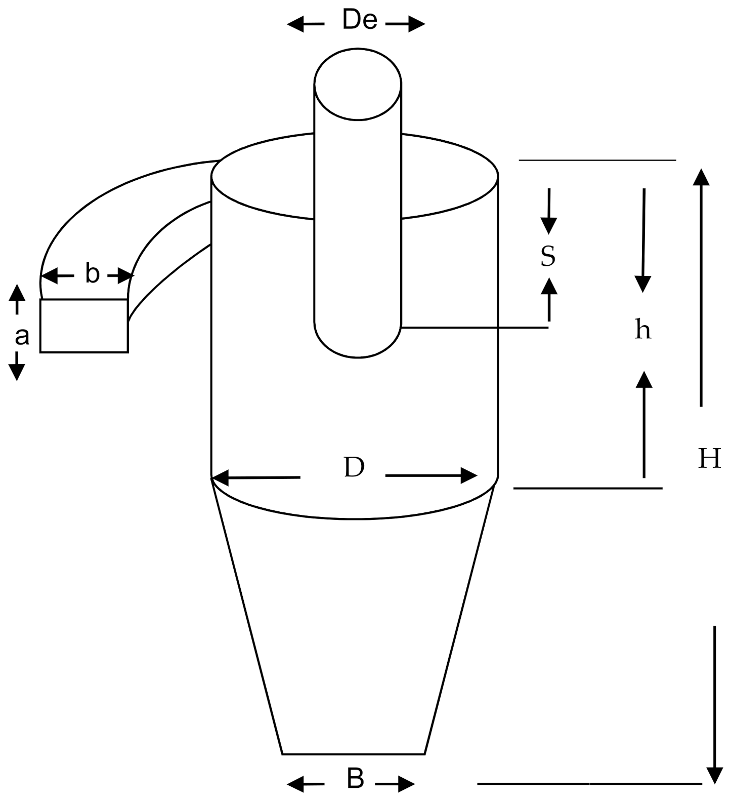
Cyclone separators are a low-cost and low-maintenance way of separating particulates from air streams. A cyclone is made up of two parts: an upper cylindrical element called the barrel and a lower conical part called the cone, as seen in
Figure 1. The air stream enters the barrel tangentially and goes downhill into the cone, generating an outer vortex. The particles are separated from the air stream by a centrifugal force caused by the increased air velocity in the outer vortex. When the air reaches the bottom of the cone, an inner vortex forms, reversing the direction of the air and exiting out the top as clean air, while particulates fall into the dust collection chamber attached to the bottom of the cyclone.
The simulation of an optimum gas cyclone with low cost is the primary focus of this research with the use of PSO, DE, and hybrid DEPSO algorithms using an objective function which is of a minimization type. The efficient global optimization is a major advantage of the DE algorithm. Furthermore, the diversity of the entire population is easily maintained throughout the process, preventing individuals from falling into a local optimum. PSO, on the other hand, has the advantage of a quick convergence speed. The best individual particle across the entire iteration is saved to obtain the lowest fitness values. Combining the benefits of DE and PSO, the use of a hybrid DEPSO strategy is proposed for this research with the goal of fast convergence and efficient global optimization. The proposed DEPSO method first reduces the search space using the DE algorithm, and then the obtained populations are used as the initial population by the PSO to achieve a fast convergence rate to a final global optimum. Moreover, DEPSO utilizes the crossover operator feature of DE to improve the distribution of information between candidates, and based on the fitness function, the hybrid algorithm can determine the global minimum cost value much better than the use of PSO alone due to its drawbacks, such as high computational complexity, slow convergence, sensitivity to parameters, and so forth.
The overview of this paper is as follows:
- -
- -
Section 4 provides insight about the DESPO algorithm.
- -
Section 5 gives a brief description about the gas cyclone device’s operation.
- -
Section 6 consists of the experimental results and performance evaluation of each algorithm.
- -
Finally,
Section 7 concludes the research work.
2. PSO
The theory behind particle swarm intelligence (PSO) is primarily nature-inspired, emulating the behaviour of animal societies by following the member of the group that is closest to the food source, such as flocks of birds and schools of fish. For example, a flock of birds during food search will follow a member of the flock that is closest to the position of the food source (the potential solution). This is achieved because of the simultaneous interactions made with each member of the flock in search of the best position. This continues until the food source is discovered (the best solution).
The PSO algorithm follows this process in search of the best solution to a given problem. The algorithm consists of a swarm of particles in which each particle is a potential solution, which usually leads to the best solution. This best solution is known as the global best and is called or.
After obtaining the two best values, the particle updates its velocity and positions with Equations (1) and (2):
where:
w is inertia;
is the particle velocity;
is the current particle (solution);
and g are defined as personal best and global best, respectively;
are random numbers between (0,1);
are learning factors;
i is the i-th particle.
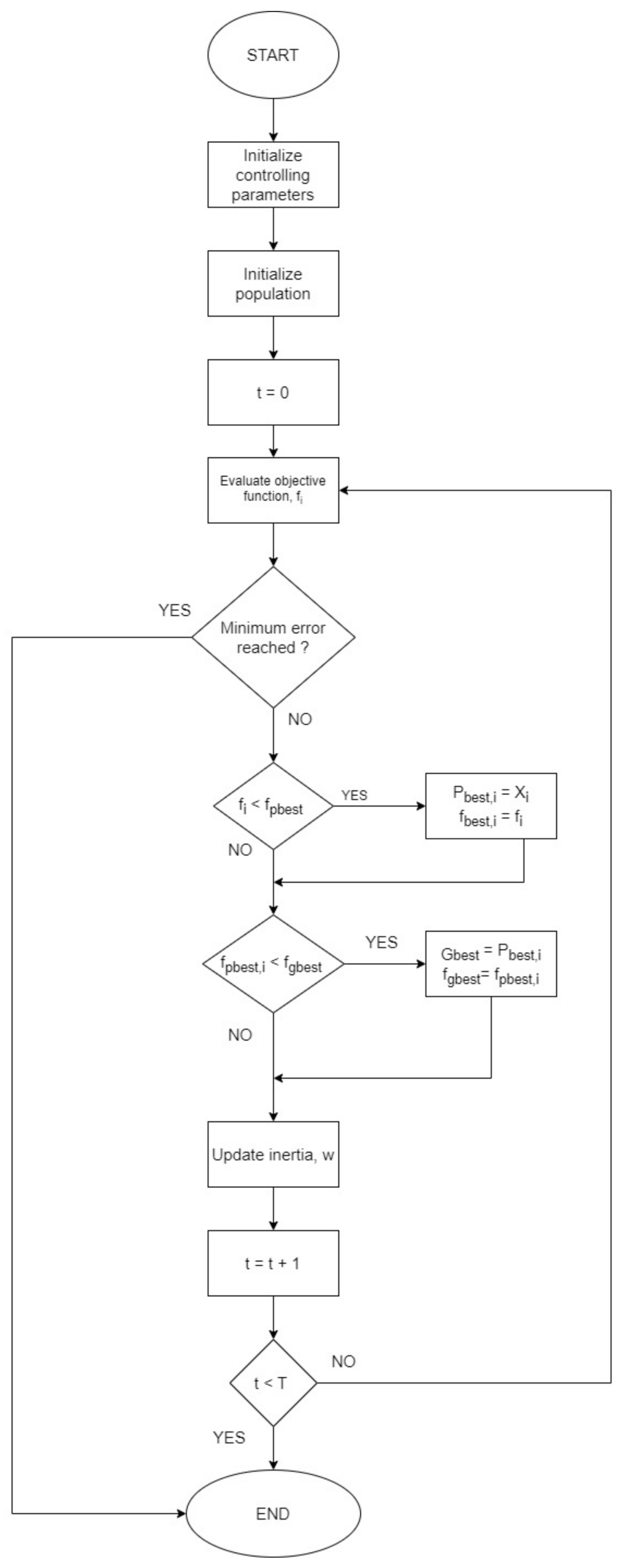
The pseudo-code (Algorithm 1) and the flowchart (see
Figure 2) of the procedure are shown below.
| Algorithm 1 PSO |
| Input: Objective function: fi; lower bound: lb; upper bound: ub; population size: Np; velocity: v; dimension size: D; termination criterion: T; inertia weight: w; learning rates: c1 and c2. |
| Output: Return gbest as the best estimation of the global optimum |
| Initialize the controlling parameters |
| Population = Initialize Population (Np,D,ub,lb,v) |
| Evaluate the objective function, fi |
| Assign Pbest as Population and fpbest as fi |
| Identify the solution with the best fitness and assign that solution as gbest and fitness as fgbest |
| for t = 0 to T |
| for i = 0 to Np |
| Calculate the velocity, vi of i-th particle |
| Calculate the new position, Xi of i-th particle |
| Bound Xi |
| Evaluate objective function fi of i-th particle |
| Update population using Xi and fi |
| if (fi < fpbest,i) then |
| Pbest,i = Xi |
| fbest,i = fi |
| end if |
| if (fPbest,i < fgbest) then |
| gbest = Pbest,i |
| fgbest = fpbest,i |
| end if |
Update Inertia, w
end for |
| end for |
4. Hybridised PSO
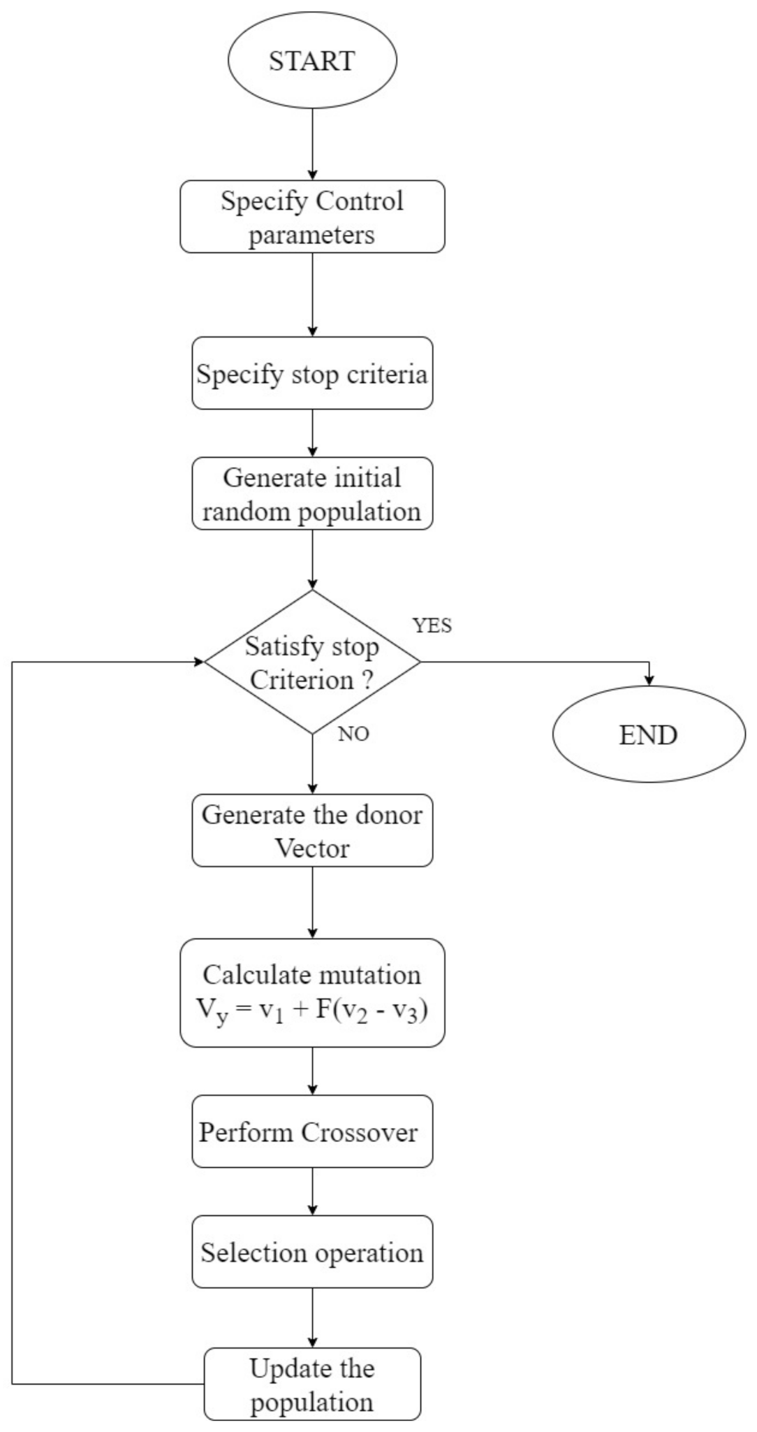
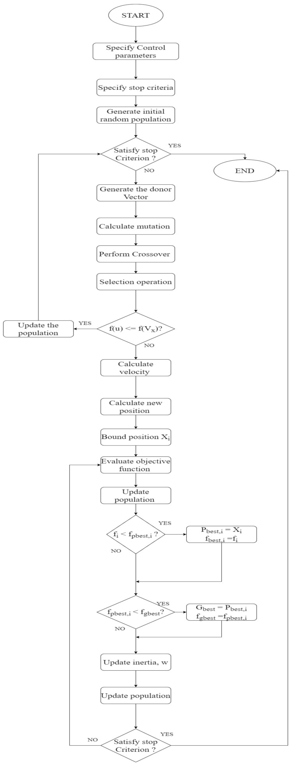
Hybridised PSO is a method that combines PSO with various classical and evolutionary optimization algorithms to make use of the strengths of both approaches while compensating for their flaws. DEPSO, a hybridised PSO which combines DE and PSO, is the suggested hybridised PSO for this research.
DEPSO follows the same steps as the standard DE method until the trial vector is created. If the trial vector meets the criteria, it is added to the population; otherwise, the algorithm moves on to the PSO phase and creates a new candidate solution. Iteratively, the technique is repeated until the optimal value is found. The incorporation of the PSO phase generates a disturbance in the population, which aids in population diversification and the output of an optimum solution. The following is an illustration of the algorithm’s procedure [
19]:
Population initialization: The individual
x, with the population number N
P, is randomly generated to form an initial population in a
D-dimensional space. All the individuals should be generated within the bounds of the solution space. The initial individuals are generated randomly in the range of the search space. Additionally, the associated velocities of all particles in the population are generated randomly in the
D-dimension space. Therefore, the initial individuals and the initial velocity can be expressed as follows [
19]:
where 1 ≤
i ≤
Np ≤
j ≤ D, [
xmin, xmax] is the range of the search space, and rand(0,1) is a random number chosen between 0 and 1.
- 2.
Iteration Loop of DE: The individual mutation operation is denoted as time
t. By randomly choosing three individuals from the previous population, the mutant individual (
t + 1) can be generated as [
19]:
where
F is a differential weight between 0 and 1.
The crossover operation aims to construct a new population
ui,(
t + 1), which is chosen from the current individuals and mutant individuals in order to increase the diversity of the generated individuals [
19]:
where rand(0, 1) is a random number chosen from 0 to 1,
jrand is an integer chosen from 1 to
D randomly, and C
r is a crossover parameter that is randomly chosen from 0 to 1.
In the selection operation, the crossover vector
U(
t+1) is compared to the target vector
Xi(
t) by evaluating the fitness function value based on a greedy criterion, and the vector with a smaller fitness value is selected as the next generation vector:
The global best part is updated with the minimum fitness value (gbest) and the personal-best part (pbest).
- 3.
Iteration Loop of PSO: The velocity and position equations of individuals remains unchanged and follows the earlier stated Equations of (1) and (2) respectively in page 3 as shown below:
The pseudo code (Algorithm 3) and flowchart (see
Figure 4) of DEPSO are shown below.
| Algorithm 3 DEPSO |
| Inputs: Fitness function: f; lb: lower bound; ub: upper bound; Np: population size; T: termination criteria; F: scaling factor/mutation rate; Pc/Cr: crossover probability; D: dimension size; w: inertia weight; learning rates: c1 and c2. |
| Output: BestVector |
| Population = Initialize Population (Np,D,ub,lb) |
| while (T ≠ True) do |
| Best_Vector = Evaluate_Population (Population) |
Vx = Select_Random_Vector (Population)
Index = Find_Index_of_Vector(V x) //Specify row number of a vector |
| Select_Random_Vector (Population, v1,v2,v3)//where v1≠ v2≠v3≠vx |
| Vy = v1 + F (v2 − v3)//donor vector |
| for (i = 0; i + +; I < D − 1)//Loop for starting Crossover |
| operation |
| if (randj[0,1] < Cr) then |
| u[i] = vx[i] |
| else u[i] = vy[i] |
| end for //end crossover operation |
| if (f(u) ≤ f(vx)) then |
| Update Population (u, Index, Population) |
| else |
| for i = 0 to Np |
| Calculate the velocity, vi of i-th particle |
| Calculate the new position, Xi of i-th particle |
| Bound Xi |
| Evaluate objective function fi of i-th particle |
| Update population using Xi and fi |
| if (fi < fpbest,i) then |
| Pbest,i = Xi |
| fbest,i = fi |
| end if |
| if (fPbest,i < fgbest) then |
| gbest = Pbest,i |
| fgbest = fpbest,i |
| Update Population (u, Index, Population) |
| end if |
| Update Inertia, w |
| end for |
| end//While loop |
| return BestVector |
5. Gas Cyclone Design
Cyclones are devices used for sizing, classification, and screening of particulate materials in mixtures with fluid (gases or liquid). Cyclones come in many sizes and shapes and have no moving parts. The mode of operation involves the process of subjecting the flowing fluid to swirl around the cylindrical part of the device. They impact the cyclone walls, fall down the cyclone wall (by gravity), and are collected in a hopper. The most important parameter of a cyclone is its collection efficiency and the pressure drop across the unit. Cyclone efficiency is increased through:
- (a)
Reduction in cyclone diameter, gas outlet diameter, and cone angle;
- (b)
Increasing the cyclone body length.
Capacity is, however, improved by increasing the cyclone diameter, inlet diameter, and body length. Increasing the pressure drop give rise to:
The design parameters include:
- -
Feed rate Q m3/s;
- -
Cyclone diameter Dc, m;
- -
Set cut size dpc, µm;
- -
Cyclone efficiency;
- -
Cyclone pressure drop, DP;
- -
Cyclone geometry (D (cyclone diameter), De(vortex finder diameter), h(cylindrical height), H(overall height), a(inlet height), b(inlet width), B(cone outlet diameter), S(vortex finder height));
- -
Temperature, °C;
- -
Pressure, N/m2;
- -
Viscosity, Ns/m2;
- -
Density fluid, kg/m3;
- -
Mass median diameter MMD, (µm);
- -
Geometric standard deviation GSD, µm;
- -
Number of cyclones;
- -
Fluid density, kg/m3;
- -
Particle density, kg/m3.
Given the cyclone geometry (as shown in
Figure 5) and the operating conditions, there are five design parameters that can be specified for a design.
These parameters are:
Cyclone geometry:
- -
a is the inlet height
- -
b is the inlet width
- -
D is the cyclone diameter
- -
De is the vortex finder diameter
- -
h is the cylindrical height
- -
B is the cone diameter
- -
H is the overall heightIt can be seen from
- -
S is the vortex finder height.
5.1. Particle Cut-Off Size DPC
According to Wang et al. [
20,
21,
22], cyclone performance depends on the geometry and operating parameters of the cyclone, as well as the particle size distribution of the entrained particulate matter. Several mathematical models have been developed to predict cyclone performance. Lapple [
23] developed a semi-empirical relationship to predict the cut point of cyclones designed according to the classical cyclone design method, where cyclone cut point is defined as the particle diameter corresponding to a 50% collection efficiency. Wang et al. showed that Lapple’s approach did not discuss the effects of particle size distribution on cyclone performance. The Lapple model was based on the terminal velocity of particles in a cyclone [
23]. From the theoretical analysis, Equation (7) was derived to determine the smallest particle that will be collected by a cyclone if it enters at the inside edge of the inlet duct:
where:
dpc (cut-point) = diameter of the smallest particle that will be collected by the cyclone if it enters on the inside edge of the inlet duct (μm);
µ = gas viscosity (kg/m/s);
b = width of inlet duct (m);
Ne = number of turns of the air stream in the cyclone;
Vi = gas inlet velocity (m/s);
= particle density (kg/m3);
= gas density (kg/m3).
5.2. Fractional Efficiency Calculation
The most important parameters in cyclone operation are pressure drop and collection efficiency. The pressure drop is given by the difference between the static pressure at the cyclone entry and the exit tube. The fractional efficiency for the
j-th particle size, according to Lapple, is given as [
23]:
where:
dpc = diameter of the smallest particle that will be collected by the cyclone with 50% efficiency,
dpj = diameter of the j-th particle.
The overall collection efficiency of the cyclone is a weighted average of the collection efficiencies for the various size ranges, namely:
where:
ɳ = overall collection efficiency;
ɳj = fractional efficiency for j-th particle size;
m = total mass of particle;
mj = mass of particle in the j-th particle size range.
5.3. Pressure Drop Calculation
The energy consumed in a cyclone is most frequently expressed as the pressure drop across the cyclone. This pressure drop is the difference between the gas static pressure measured at the inlet and outlet of the cyclone. Many models have been developed to determine this pressure drop. Some of the commonly used equations to calculate the pressure drop are:
- (a)
The Koch and Licht Pressure Drop Equation.
Koch and Licht (1977) expressed the cyclone pressure drop as
where:
g = gas density (lbm/ft3);
Vi = inlet velocity (ft/s);
N
Π = number of velocity heads (inches of water) and is expressed as
K = 16 for no inlet vane 7.5 with neutral inlet vane;
a, b = inlet height and width, respectively.
- (b)
The Ogawa Equation.
Another pressure drop equation due to Ogawa (1984) takes the form of
The prediction of the performance of the cyclone separators is a challenging problem for the designers owing to the complexity of the internal aerodynamic process and dust particles. Hence, modern numerical simulations are needed to solve this problem. Fluid flows have long been mathematically described by a set of nonlinear, partial differential equations, namely the Navier–Stokes equations.
A cyclone is required to remove carbon dust particles from affluent air coming from a thermal power station at a rate of 5.0 m3/s at 65 °C. The dust particles are assumed to have a normal size distribution with an MMD of 20 µm and a GSD of 1.5 µm. For energy cost consideration, the pressure drop in the cyclone is required to be not more than 1000 N/m2. The density of the dust particle is 2250 kg/m3, and the cyclone is operating at atmospheric pressure. To attain overall efficiency of 70% and above, the recommended required geometry/size and cut size of the cyclone are: Q = 5 m3/s, temp = 65 °C, MMD = 20 µm, GSD = 15 µm, pressure 1000 N/m2, and ρ dust particle = 2250 kg/m2.
This study develops PSO, DE, and DEPSO models for the design optimization of a 5.0 m3/s gas cyclone instrument.
6. Results and Discussion
The cost of the operation of a gas cyclone is the primary problem set for this research, instead of using two conflicting objective functions, namely efficiency and pressure drop. In general, the total cost per unit will be a function of a fixed cost cyclone and the energy cost of operating the cyclone:
Ct = Fixed cost + energy cost.
Assuming the cost of the cyclone depends on its diameter, the fixed cost can be expressed as
where:
f is an investment factor to allow for installation;
Dc is the cyclone diameter;
Ne is number of turns of the air stream in the cyclone;
H is the time worked per year;
Y is the number of years.
The energy cost is given by
where:
Q is the feed rate (m3/s);
∆P is the pressure drop (Pa);
Ce is cost per unit energy.
β1 = [dpc2(ρs − ρf)ΠNtNeQ/9aobo2 µN]2/3;
β2 = [dpc2(ρs − ρf)ΠNtQ/9aobo2 µN]−4/3.
The objective function is of a minimization type, and the EC methods search for an optimized cyclone geometry with low cost per unit. Using the table of parameters as shown in
Table 1,
Table 2,
Table 3,
Table 4,
Table 5,
Table 6,
Table 7,
Table 8 and
Table 9, the cost performance and overall efficiency of each of the algorithms are shown in the figures below.
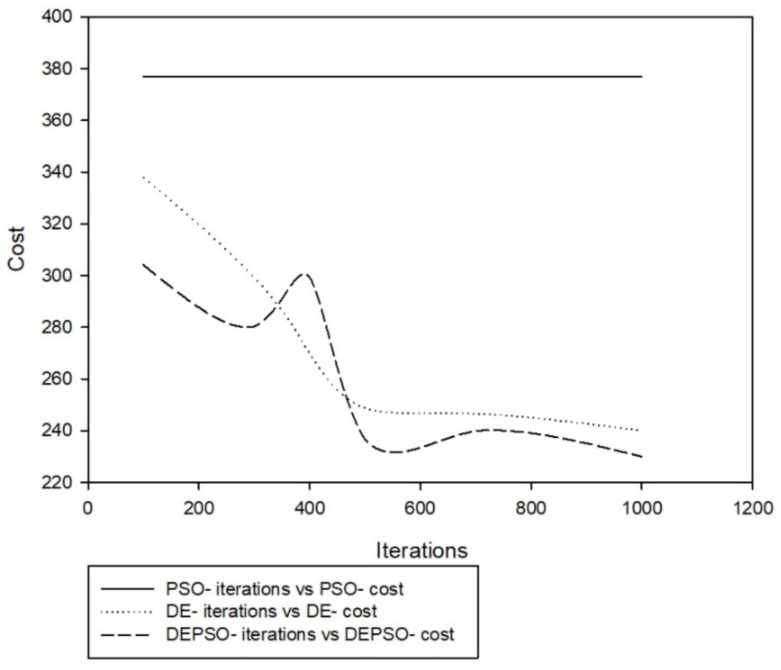
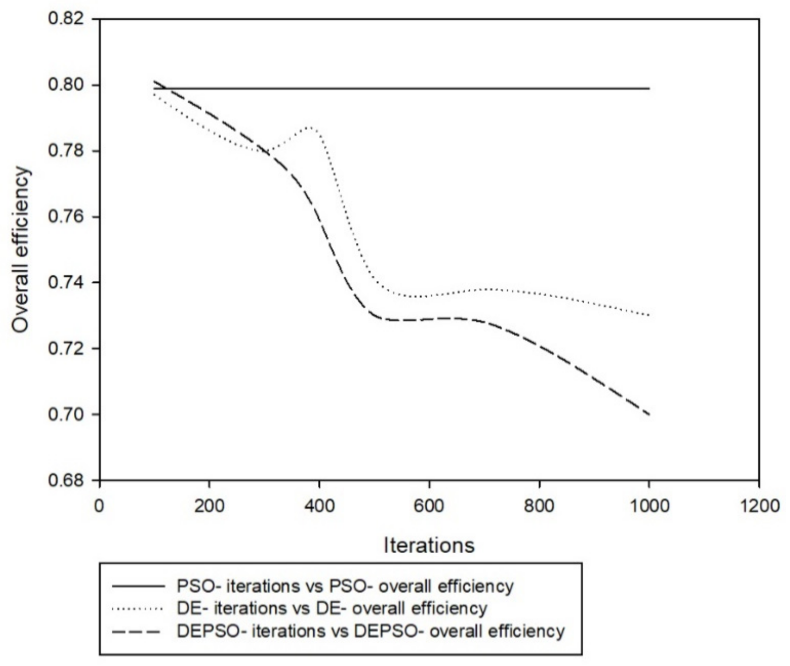
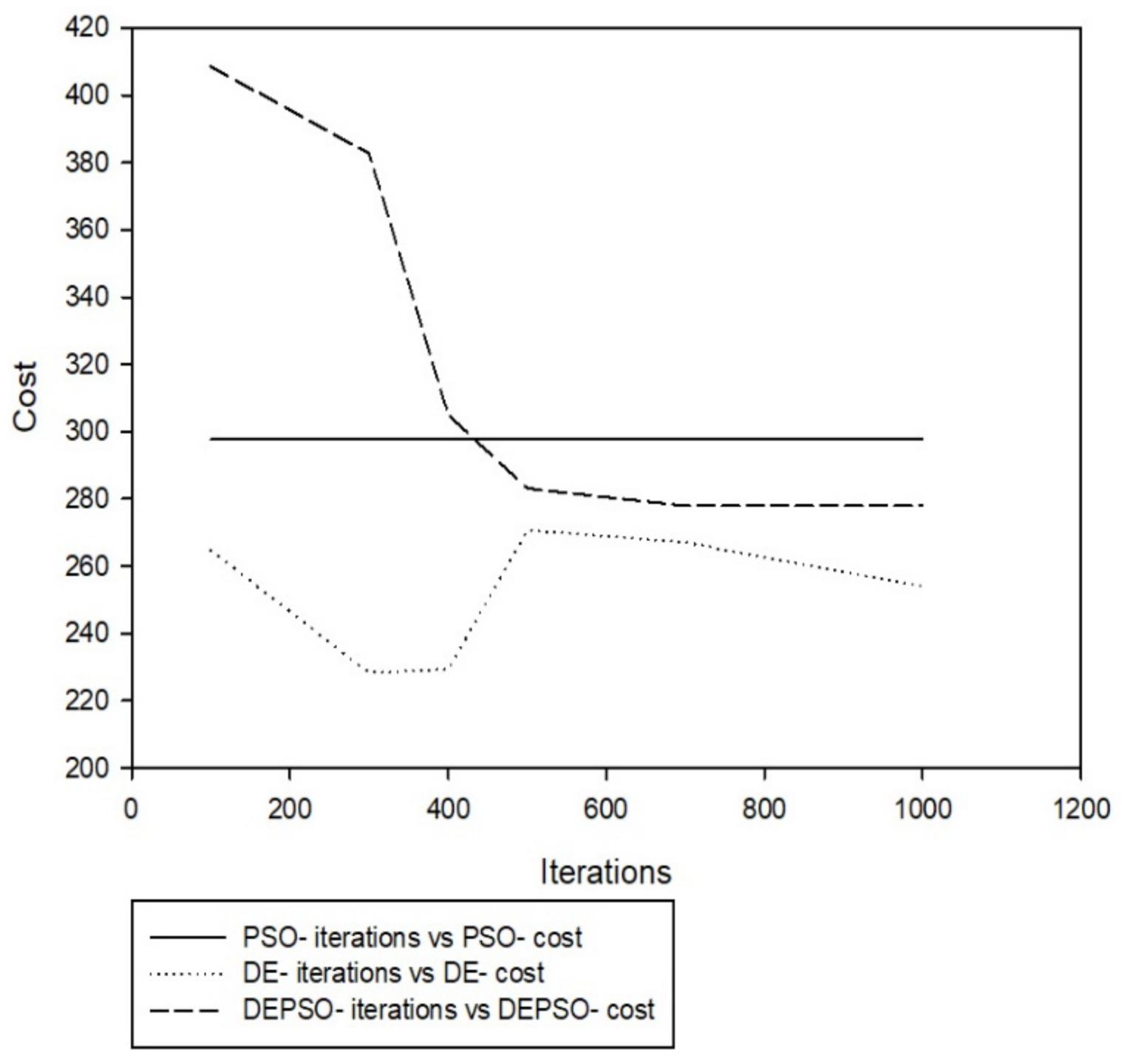
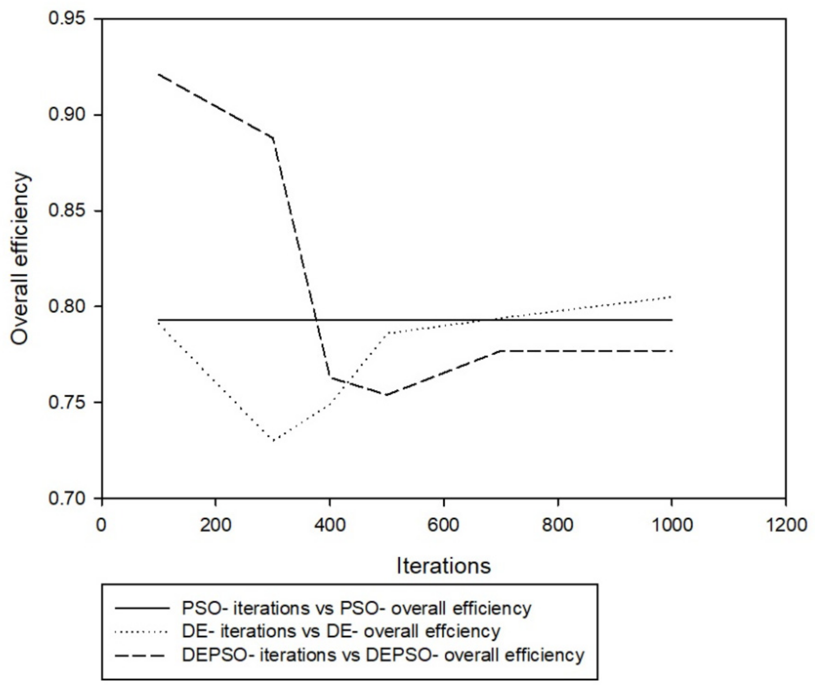
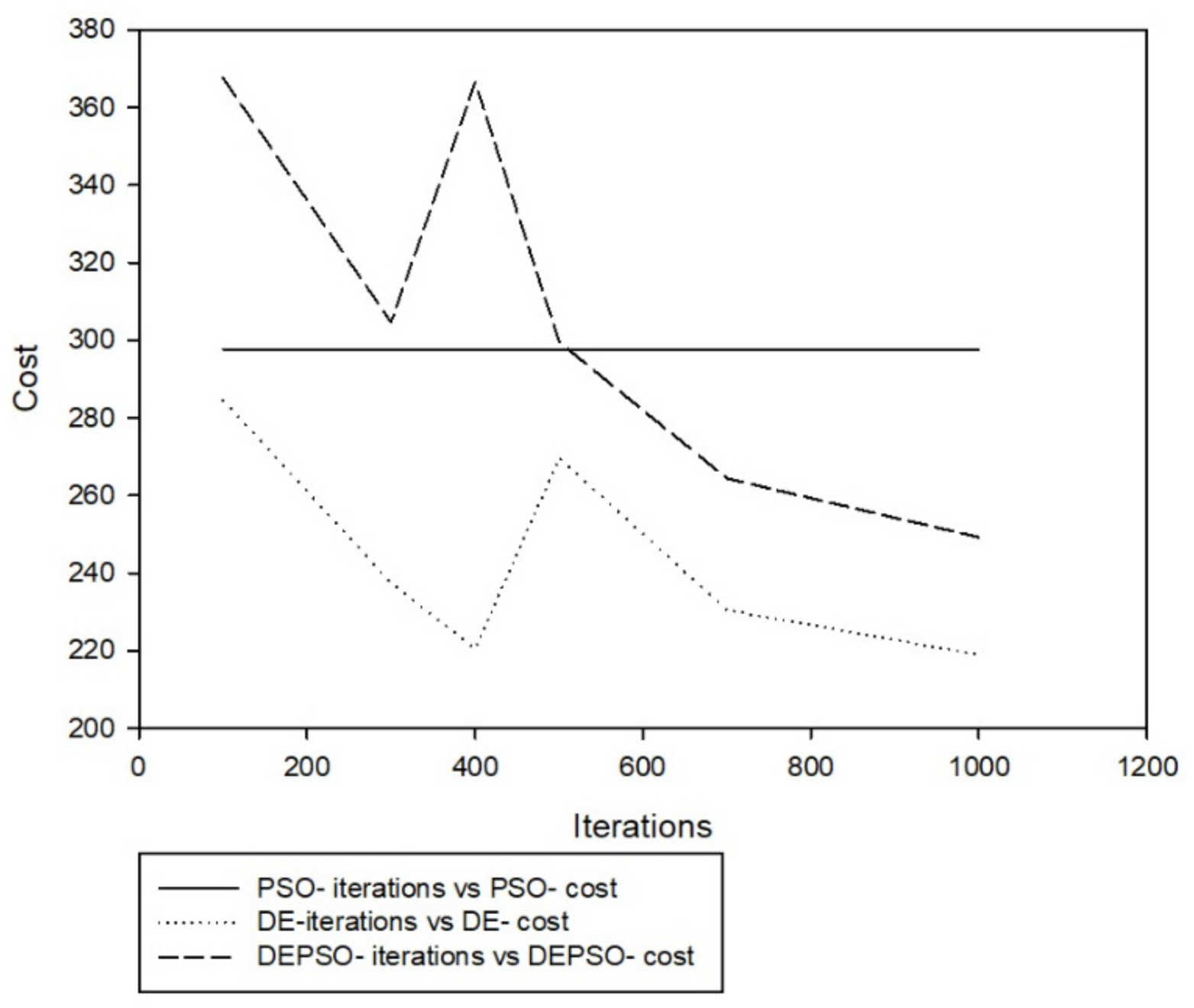
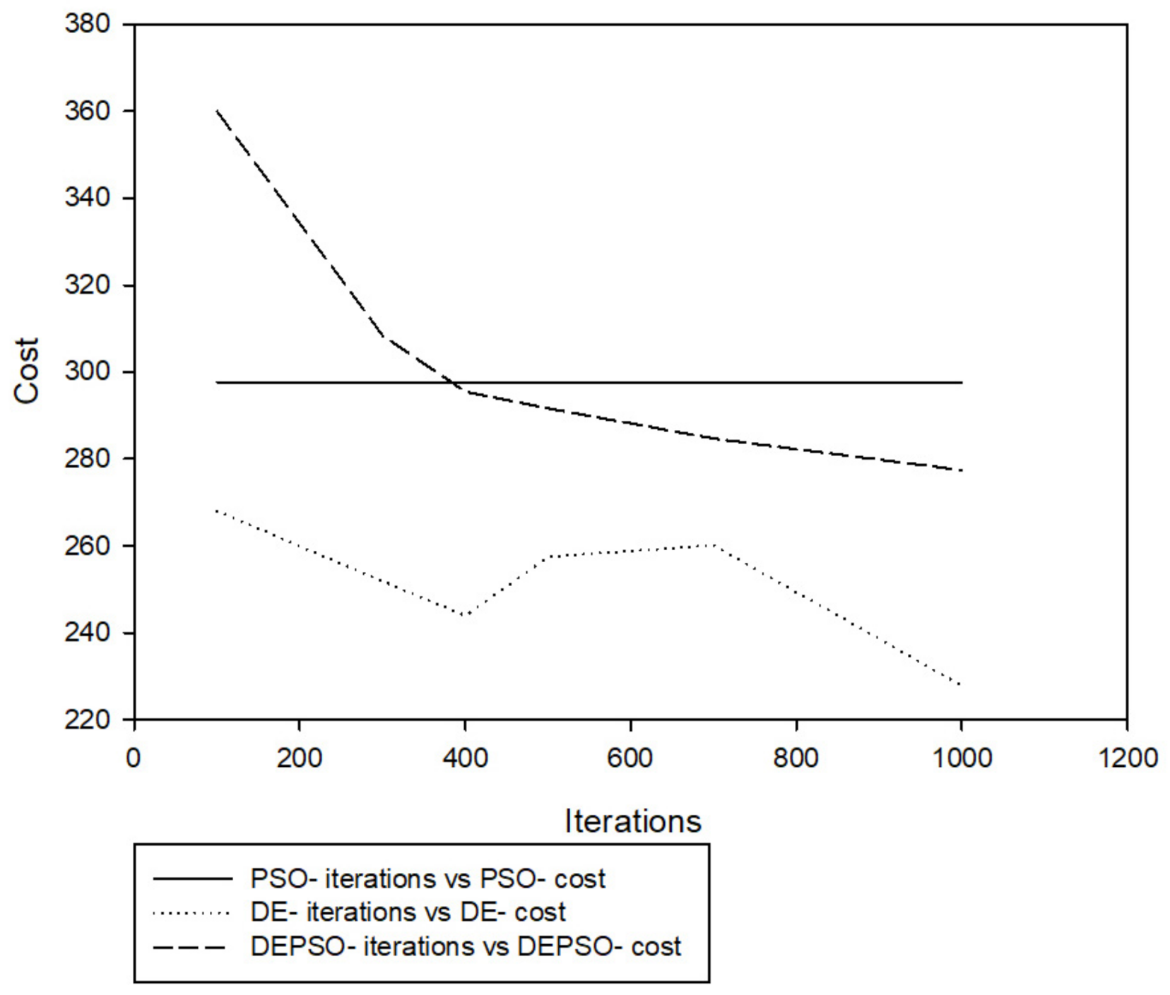
The following can be observed from the plots and tables below:
It can be seen from
Table 10 that DEPSO at 1000 iterations with a particle size of 40 has a cost-effective value of 230 naira/s, with an overall efficiency of 0.70.
It can also be seen from
Table 10 and
Figure 6,
Figure 7,
Figure 8,
Figure 9,
Figure 10,
Figure 11,
Figure 12,
Figure 13,
Figure 14,
Figure 15,
Figure 16,
Figure 17,
Figure 18 and
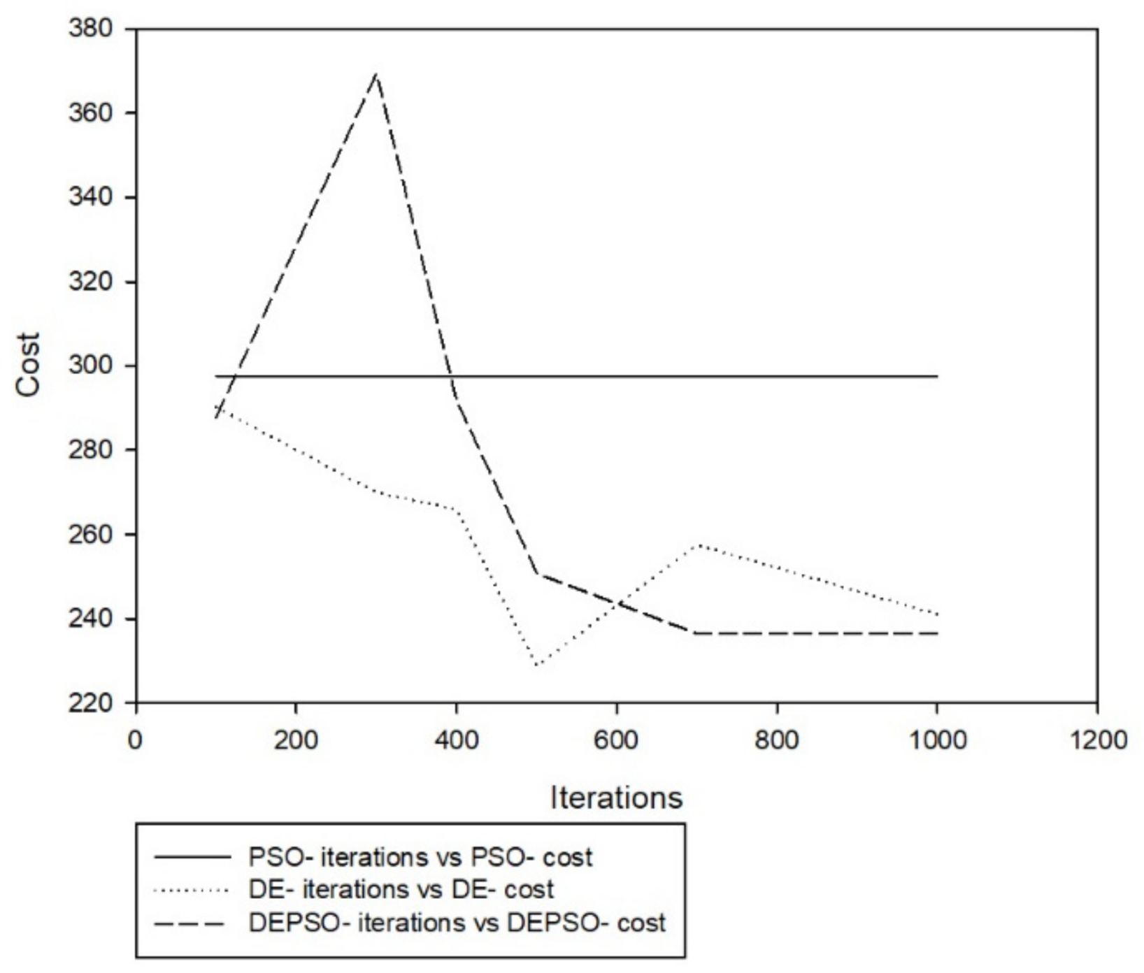
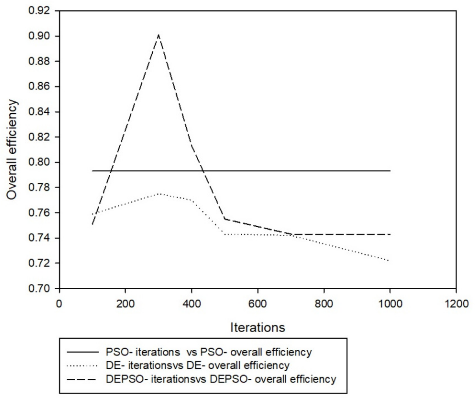
Figure 19 that the PSO algorithm fails to provide any reasonable results when applied to complex optimization problems, due to its premature convergence, high computational complexity, slow convergence, sensitivity to parameters, and so forth. DEPSO solves this issue by utilizing the crossover operator of DE to improve the distribution of information between candidate solutions.
In terms of the best efficiency at low cost for DE algorithm, at a particle size of 60 at 400 iterations, its cost and overall efficiency are 229.365 naira/s and 0.749, respectively, as shown in
Figure 10 and
Figure 11.
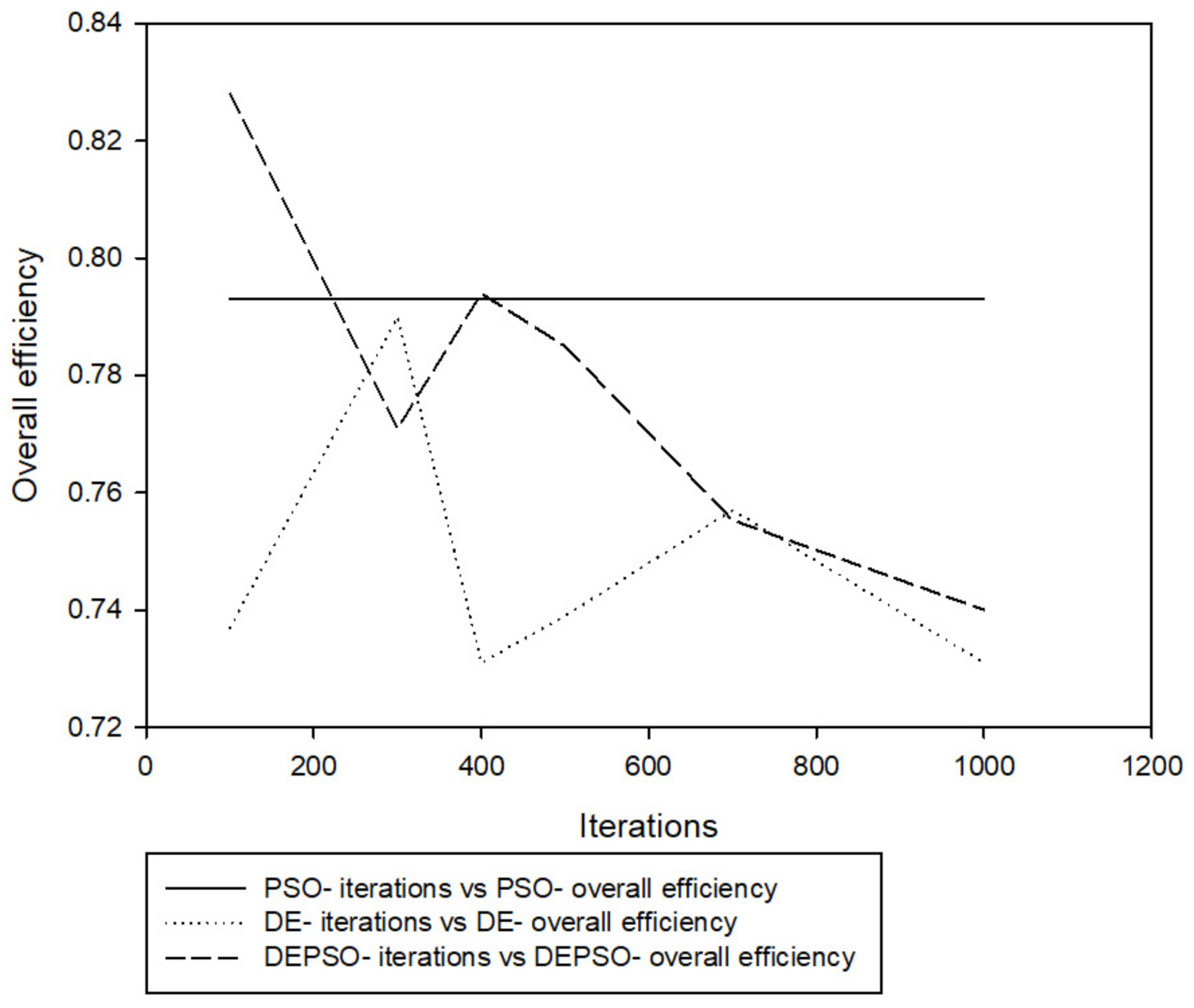
In terms of the best efficiency at a low cost for the DEPSO algorithm, at a particle size of 70 at 1000 iterations, its cost and overall efficiency are 249.192 naira/s and 0.786, respectively, as shown in
Figure 12 and
Figure 13.
As seen from
Table 10, the DE algorithm’s lowest cost is 218.938 naira/s with an overall efficiency of 0.716.
Table 1.
Cyclone input data.
Table 1.
Cyclone input data.
| Parameters | Value |
|---|
| Feed rate, Q | 5.0 |
| Particle size 1 | 0.00002 |
| Particle size 2 | 0.0000015 |
| Particle Density | 2250 |
| Viscosity | 0.00002039 |
| Delta pressure | 1000 |
| Particle mass 1 | 0.000056 |
| Particle mass 2 | 0.000042 |
| Number of particle range | 1 |
| Assumed natural length | 2.078 |
Table 2.
Investment/cost data.
Table 2.
Investment/cost data.
| Parameters | Value |
|---|
| Investment factor | 3.9 |
| Number of years | 10 |
| Period of operation/year, (seconds) | 0.0000015 |
| Cost/square m of cyclone | 20.5 |
| Number of cyclone | 1 |
Table 3.
Parameters list with 40-particle size.
Table 3.
Parameters list with 40-particle size.
| Parameters | Value |
|---|
| Particle size | 40 |
| Dimensions | 7 |
| Probability of crossover range, Cr | 0.5 |
| Scaling factor | 1.0 |
| w | 0.729 |
| c1 | 2 |
| c2 | 2 |
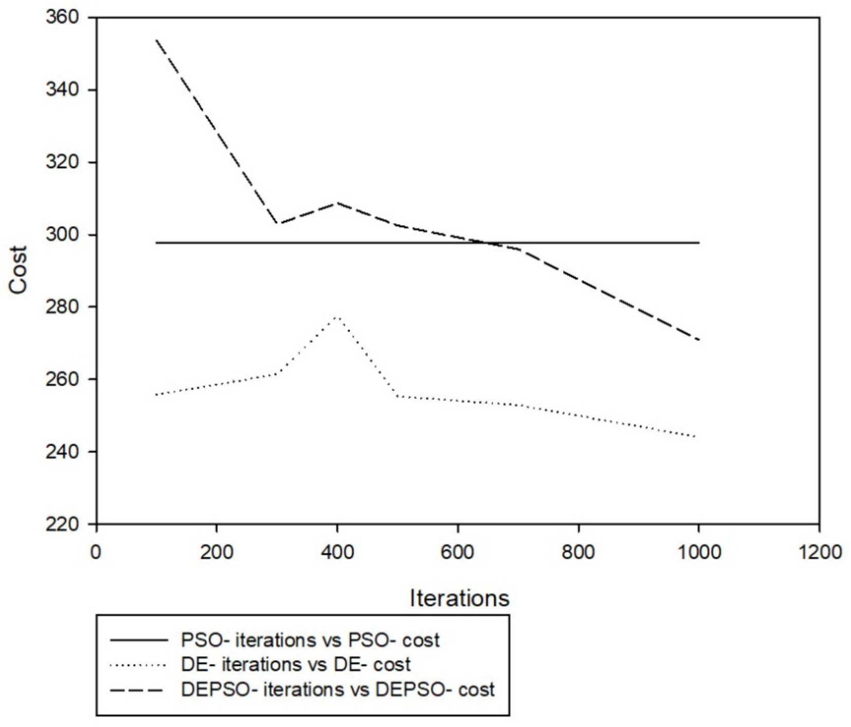
Figure 6.
Cost performance of DE, DEPSO, and PSO algorithms at 40 particles.
Figure 6.
Cost performance of DE, DEPSO, and PSO algorithms at 40 particles.
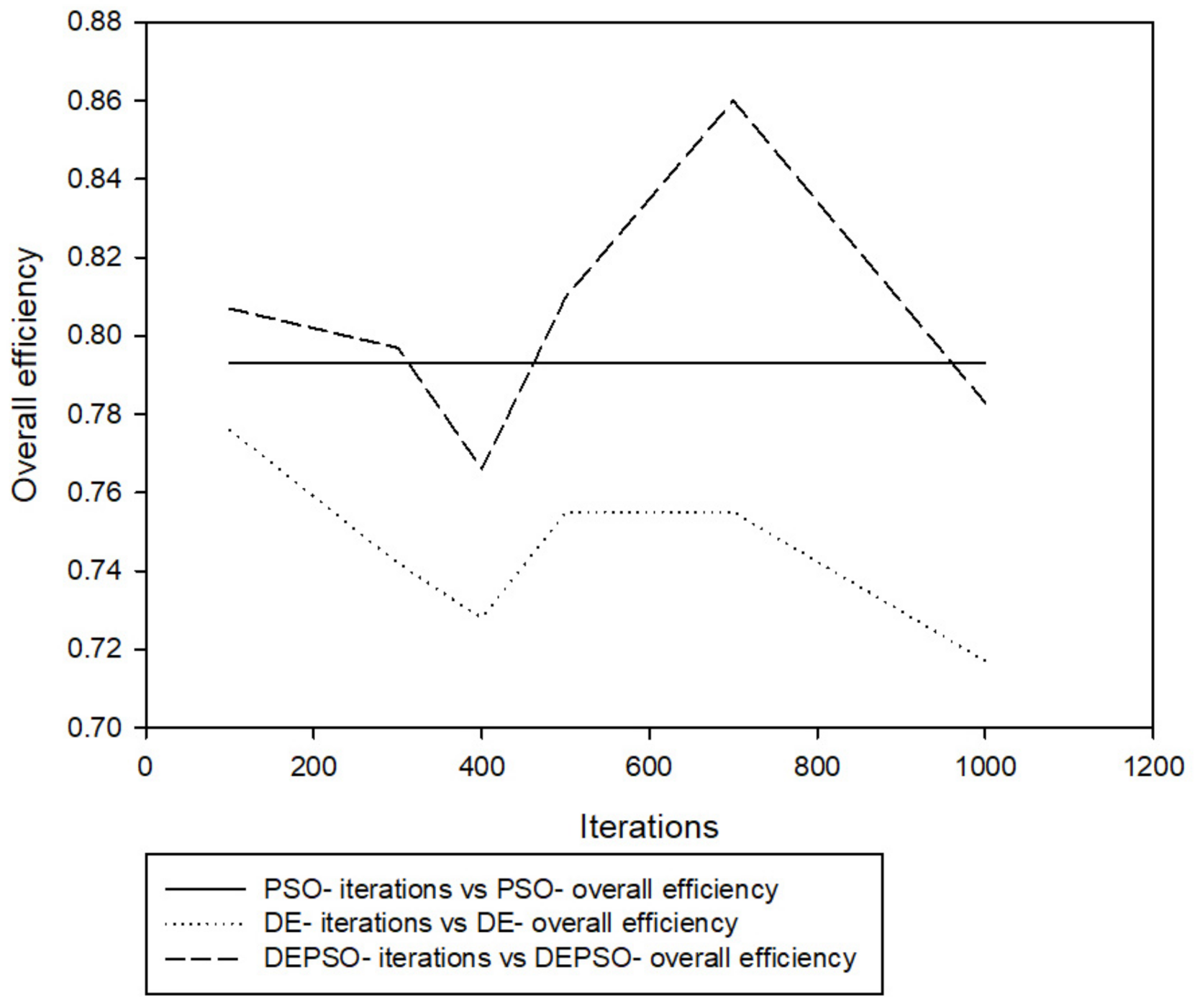
Figure 7.
Overall efficiency of DE, DEPSO, and PSO algorithms at 40 particles.
Figure 7.
Overall efficiency of DE, DEPSO, and PSO algorithms at 40 particles.
Table 4.
Parameters list with 50-particle size.
Table 4.
Parameters list with 50-particle size.
| Parameters | Value |
|---|
| Particle size | 50 |
| Dimensions | 7 |
| Probability of crossover range, Cr | 0.5 |
| Scaling factor | 1.0 |
| w | 0.729 |
| c1 | 2 |
| c2 | 2 |
Figure 8.
Cost performance of DE, DEPSO, and PSO algorithms at 50 particles.
Figure 8.
Cost performance of DE, DEPSO, and PSO algorithms at 50 particles.
Figure 9.
Overall efficiency of DE, DEPSO, and PSO algorithms at 50 particles.
Figure 9.
Overall efficiency of DE, DEPSO, and PSO algorithms at 50 particles.
Table 5.
Parameters list with 60-particle size.
Table 5.
Parameters list with 60-particle size.
| Parameters | Value |
|---|
| Particle size | 60 |
| Dimensions | 7 |
| Probability of crossover range, Cr | 0.5 |
| Scaling factor | 1.0 |
| W | 0.729 |
| c1 | 2 |
| c2 | 2 |
Figure 10.
Cost performance of DE, DEPSO, and PSO algorithms at 60 particles.
Figure 10.
Cost performance of DE, DEPSO, and PSO algorithms at 60 particles.
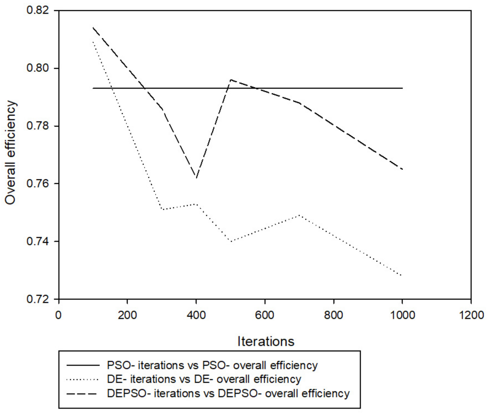
Figure 11.
Overall efficiency of DE, DEPSO, and PSO algorithms at 60 particles.
Figure 11.
Overall efficiency of DE, DEPSO, and PSO algorithms at 60 particles.
Table 6.
Parameters list with 70-particle size.
Table 6.
Parameters list with 70-particle size.
| Parameters | Value |
|---|
| Particle size | 70 |
| Dimensions | 7 |
| Probability of crossover range, Cr | 0.5 |
| Scaling factor | 1.0 |
| w | 0.729 |
| c1 | 2 |
| c2 | 2 |
Figure 12.
Cost performance of DE, DEPSO, and PSO algorithms at 70 particles.
Figure 12.
Cost performance of DE, DEPSO, and PSO algorithms at 70 particles.
Figure 13.
Overall efficiency of DE, DEPSO, and PSO algorithms at 70 particles.
Figure 13.
Overall efficiency of DE, DEPSO, and PSO algorithms at 70 particles.
Table 7.
Parameters list with 80-particle size.
Table 7.
Parameters list with 80-particle size.
| Parameters | Value |
|---|
| Particle size | 80 |
| Dimensions | 7 |
| Probability of crossover range, Cr | 0.5 |
| Scaling factor | 1.0 |
| w | 0.729 |
| c1 | 2 |
| c2 | 2 |
Figure 14.
Cost performance of DE, DEPSO, and PSO algorithms at 80 particles.
Figure 14.
Cost performance of DE, DEPSO, and PSO algorithms at 80 particles.
Figure 15.
Overall efficiency of DE, DEPSO, and PSO algorithms at 80 particles.
Figure 15.
Overall efficiency of DE, DEPSO, and PSO algorithms at 80 particles.
Table 8.
Parameters list with 90-particle size.
Table 8.
Parameters list with 90-particle size.
| Parameters | Value |
|---|
| Particle size | 90 |
| Dimensions | 7 |
| Probability of crossover range, Cr | 0.5 |
| Scaling factor | 1.0 |
| w | 0.729 |
| c1 | 2 |
| c2 | 2 |
Figure 16.
Cost performance of DE, DEPSO, and PSO algorithms at 90 particles.
Figure 16.
Cost performance of DE, DEPSO, and PSO algorithms at 90 particles.
Figure 17.
Overall efficiency of DE, DEPSO, and PSO algorithms at 90 particles.
Figure 17.
Overall efficiency of DE, DEPSO, and PSO algorithms at 90 particles.
Table 9.
Parameters list with 100-particle size.
Table 9.
Parameters list with 100-particle size.
| Parameters | Value |
|---|
| Particle size | 100 |
| Dimensions | 7 |
| Probability of crossover range, Cr | 0.5 |
| Scaling factor | 1.0 |
| w | 0.729 |
| c1 | 2 |
| c2 | 2 |
Figure 18.
Cost performance of DE, DEPSO, and PSO algorithms at 100 particles.
Figure 18.
Cost performance of DE, DEPSO, and PSO algorithms at 100 particles.
Figure 19.
Overall efficiency of DE, DEPSO, and PSO algorithms at 100 particles.
Figure 19.
Overall efficiency of DE, DEPSO, and PSO algorithms at 100 particles.
Table 10.
Lowest cost value.
Table 10.
Lowest cost value.
| | PSO | DE | DEPSO |
|---|
| | Cost | Overall Efficiency | Cost | Overall Efficiency | Cost | Overall Efficiency |
| | 297.715 | 0.793 | 218.938 | 0.716 | 230 | 0.70 |
| Iteration Number | 100–1000 | 1000 | 1000 |
| Particle Size | 50–100 | 70 | 40 |
Table 11.
PSO parameters used for design parameter optimization.
Table 11.
PSO parameters used for design parameter optimization.
| Parameters | Value |
|---|
| Maximum iteration | 1000 |
| Particle size | 50 |
| Dimensions | 7 |
| Probability of crossover range, Cr | 0.5 |
| Scaling factor | 1.0 |
| w | 0.729 |
| c1 | 2 |
| c2 | 2 |
Table 12.
DE parameters used for design parameter optimization.
Table 12.
DE parameters used for design parameter optimization.
| Parameters | Value |
|---|
| Maximum iteration | 1000 |
| Particle size | 70 |
| Dimensions | 7 |
| Probability of crossover range, Cr | 0.5 |
| Scaling factor | 1.0 |
| w | 0.729 |
| c1 | 2 |
| c2 | 2 |
Table 13.
DEPSO Parameters used for design parameter optimization.
Table 13.
DEPSO Parameters used for design parameter optimization.
| Parameters | Value |
|---|
| Maximum iteration | 1000 |
| Particle size | 40 |
| Dimensions | 7 |
| Probability of crossover range, Cr | 0.5 |
| Scaling factor | 1.0 |
| w | 0.729 |
| c1 | 2 |
| c2 | 2 |
Table 14.
Design parameters.
Table 14.
Design parameters.
| Design Parameters are in the Ratio of Dc | Analytical Method (Stairmand Model) | PSO | DE | Hybrid DEPSO |
|---|
| Overall cyclone height | 4.0 | 3.925 | 3.371 | 3.884 |
| Inlet height, ao | 0.5 | 0.491 | 0.494 | 0.489 |
| Gas outlet diameter, Deo | 0.5 | 0.168 | 0.411 | 0.309 |
| Cylindrical height of cyclone, ho | 1.5 | 0.977 | 0.817 | 1.006 |
| Inlet width, bo | 0.2 | 0.213 | 0.242 | 0.209 |
| Gas outlet length, So | 0.5 | 0.674 | 1.177 | 1.171 |
| Dust outlet diameter, Bo | 0.375 | 0.485 | 0.447 | 0.179 |
| Pressure drop (Pa) | 1000 | 469.034 | 364.668 | 493.24 |
| Inlet velocity m/s | 19.86 | 11.066 | 9.706 | 11.36 |
| Cut size dpc (µm) | 8.67855 × 10⁻⁶ | 1.021 × 10⁻⁵ | 1.26 × 10⁻⁵ | 9.96 × 10⁻⁶ |
| Cost/s (Naira/s) | - | 297.715 | 218.938 | 230 |
| Overall efficiency | 0.890 | 0.793 | 0.716 | 0.70 |
| Particle size | - | 50 | 70 | 40 |
The following can be observed in
Table 14 above:
Due to the problem of being a minimization type, each algorithm’s efficiency is lower compared to the Stairmand’s model. The pressure drop of DE is the lowest, followed by PSO and DEPSO. Moreover, each algorithm’s pressure drop is considerably lower than the Stairmand’s model. An increase in pressure drop will lead to an increase in separation efficiency, higher capacity, and cleaner overflow.
Another factor that leads to lower efficiency is the inlet velocity of the cyclone; as seen in
Table 14 above, all algorithms have a lower inlet velocity when compared to the Stairmand’s model. An increase in inlet velocity leads to an increase in separation efficiency, thereby leading to an increase in the overall efficiency, because of higher resultant centrifugal force.


