Genetic Algorithm Based Deep Learning Neural Network Structure and Hyperparameter Optimization

Abstract

Alzheimer’s disease is one of the major challenges of population ageing, and diagnosis and prediction of the disease through various biomarkers is the key. While the application of deep learning as imaging technologies has recently expanded across the medical industry, empirical design of these technologies is very difficult. The main reason for this problem is that the performance of the Convolutional Neural Networks (CNN) differ greatly depending on the statistical distribution of the input dataset. Different hyperparameters also greatly affect the convergence of the CNN models. With this amount of information, selecting appropriate parameters for the network structure has became a large research area. Genetic Algorithm (GA), is a very popular technique to automatically select a high-performance network architecture. In this paper, we show the possibility of optimising the network architecture using GA, where its search space includes both network structure configuration and hyperparameters. To verify the performance of our Algorithm, we used an amyloid brain image dataset that is used for Alzheimer’s disease diagnosis. As a result, our algorithm outperforms Genetic CNN by $11.73\%$ on a given classification task.

1. Introduction

Alzheimer’s disease (AD) is the most common cause of dementia, and is one of the major problems of global population ageing. With advances in relevant technologies, there is ongoing research into the diagnosis and treatment of dementia.

Amyloid, as well as the tau ($\tau$) protein, is considered as one of the main causes of AD because this protein is found in brains of the majority of patients with AD. Moreover, as deposition of amyloid occurs gradually and long before the disease is clinically significant, it is regarded as a very important factor of screening for AD [1].

Standard Uptake Value Ratio (SUVR) [2], is a classical, quantitative analysis method, to analyse Positron Emission Tomography-Computed Tomography (PET/CT). This method calculates the ratio of two mean activity concentrations of Region of Interest (RoI) or Volume of Interest (VoI), and the reference region. These activity concentrations are calculated using the intensity of the image, which has been regularised using patients’ body weight and injected radioactivity. SUVR provides an objective and quantitative update ratio. However, it is very difficult to decide RoI/VoI and takes a long time to analyse. Furthermore, generalising the threshold for the diagnosis is impossible due to the noise and inconsistency of devices.

Recently, with the development of image processing techniques, various deep learning-based technologies are applied across different areas of medical industry [3,4]. Specifically, image classification techniques extract relevant features from input images via training, and use these features to perform classification.

If an appropriate algorithm is used for the given domain, a strong performance is observed. However, depending on the statistical distribution of the input data, the error space formed by the loss function is completely different. Therefore, various optimisation techniques are required. Zoph et al. [5] suggested a machine learning-based method to search for the best network structure for an input data. It decides the ideal structure for each layer using the information from previous hidden layers.

Genetic Algorithm (GA) [6] is a computational model that simulates methodologies described from Darwin’s theory of evolution, such as natural selection and genetic mechanisms. As GA searches the optimal solution through simulation of the natural evolution process, it is beneficial to use this algorithm for problems that require complicated algorithms to find their solutions. Genetic CNN [7] is a popular example that is developed from GA, which optimises the structure of CNN models. Network structure configured from the algorithm showed similar performances when compared with state-of-the-art classification networks.

However, one limitation of Genetic CNN is that it does not consider a set of hyperparameters, which affects the rate of convergence of the network on the error surface. Examples of such hyperparameters include activation functions and optimisation algorithms. Appropriate selection of these parameters will lead to faster convergence to the global minimum point on the error surface. This leads to excellent task performance, and also avoids problems such as overfitting.

In this paper, we show that our version of genetic algorithm is capable of finding the best-performing CNN architecture, including activation function and optimisation algorithm, which is specific for the given input dataset. The input dataset used in the algorithm is the set of PET/CT images with amyloid. As these images are used for early diagnosis of AD, the dataset is appropriate for extracting features of lesions associated with AD.

2. Related Works

2.1. Convolutional Neural Networks

A Convolutional Neural Network (CNN) [8] is a type of multilayer perceptron that originates from the behaviour of the visual nervous system of animals. Due to its nature, networks with layers of CNN outperform other type of layers, such as Bag of Visual Words, for tasks involving visual features.

CNN models consist of a convolution layer, activation layer, pooling layer, and fully connected layer. Figure 1 visualises the structure of a basic CNN model. The convolution layer involves convolution filtering of input images to extract feature maps, and the activation layer introduces non-linearity to these feature maps. Non-linearity is important in neural networks because it adds complexity to the network, which allows the network to learn complex, non-linear classifiers for the input data. The pooling layer abstracts these feature maps and changes the dimension of them if required. Finally, the fully connected layer uses information obtained from the convolution and pooling layers to perform classification.

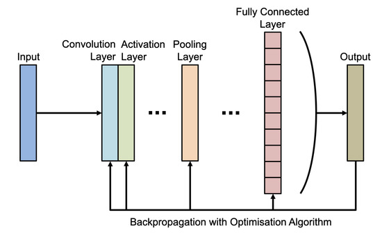
Figure 1. Basic structure of a typical Convolutional Neural Network (CNN).

To find the best combination of parameters that minimises the loss function (or the cost function) of the model, an optimisation algorithm is used. This algorithm updates parameters of the CNN during the backpropagation process.

Outputs of the fully connected layer are usually represented as a linear combination of input and weights, as shown in (1).

$${\widehat{y}}_j=f\left(\sum _{i=0}^n{w}_{i,j}{x}_i,b_j\right)$$

(1)

where ${\widehat{y}}_j$ is the output, $x_i$ is the input, $b_j$ is bias, and $w_{i,j}$ is the weight of the fully connected layer. f is an activation function.

Typical cost function for optimising fully connected networks is Mean Squared Error (MSE).

$$J\left(w_{i,j}\right)=E\left[e^2\left(t\right)\right]=E\left[{(y_j-{\widehat{y}}_j)}^2\right]$$

(2)

where $y_j$ is the ground truth value and $J\left(\right)$ represents a loss or cost function.

Optimisation of the weight is often done using Gradient Descent (GD) [9] technique (3,4).

$${\mathbf{w}}_{\mathbf{t}+\mathbf{1},\mathbf{j}}={\mathbf{w}}_{\mathbf{t},\mathbf{j}}-\eta \frac{\partial J{\mathbf{w}}_{\mathbf{t},\mathbf{j}}}{\partial {\mathbf{w}}_{\mathbf{t},\mathbf{j}}}$$

(3)

$$\frac{\partial J{\mathbf{w}}_{\mathbf{t},\mathbf{j}}}{\partial {\mathbf{w}}_{\mathbf{t},\mathbf{j}}}=-2(y_{t,i}-{\widehat{y}}_{t,i}){\mathbf{x}}_{\mathbf{t},\mathbf{i}}$$

(4)

where $\eta$ is a learning rate.

As shown in (4), the optimisation algorithm is heavily affected by the input of the layer. Furthermore, the output of the layer has been processed with an activation function. Therefore, proper selection of both activation function and optimisation algorithm is essential for the performance of the network.

The cost function, as a result of the relationship between input data and parameters of the network, defines an error surface. Figure 2 represents a simple error surface defined by the cost function. This surface affects the accuracy and convergence speed of the network. Therefore, input data does effect the performance of the neural networks significantly, and good architectural design is required to ensure this performance.

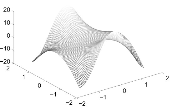
Figure 2. Example error surface defined by the cost function, input dataset and parameters of the network.

Recently, several CNN structures have been investigated to achieve better performance, specially for the classification tasks. These structures can be categorized into three types; Chain-shaped; Multiple-path; and Highway Network. A chain-shaped network is a simple, linear structure that is used from the beginning of CNNs. Still, many state-of-the-art networks, such as VGG [10], perform very well with this structure. Multiple-Path Networks increase the number of layers that are connected in parallel, and concatenate or add the results of these layers as the input for the next layer. ResNet [11] and GoogleNet [12] are popular examples of this block. Finally, highway network [13] uses the output of a layer as input for all proceeding layers. DenseNet [14] is a very popular network that successfully adapts this network structure.

2.2. Hyperparameters

As mentioned in the previous section, activation function and optimisation algorithm are the core components of the CNN. In addition, these hyperparameters will increase the convergence speed of the model, and greatly change the score of the models by avoiding overfitting [15] and vanishing gradient problems [16].

The activation function is used to introduce non-linearity to the network. Various activation functions are suggested. Rectifier Linear Unit (ReLU) [17], which is derived from the action potential of neurons, is one of the most popular activation functions. As ReLU outputs all negative numbers to zero, negative nodes will die out. In order to solve this problem (dying ReLU), Leaky ReLU [18] is introduced. In this function, negative values are multiplied with a small parameter, $\alpha$, and not zeroed out. Finally, Clipped Relu [19] is introduced in order to prevent the exploding gradient problem of ReLU. It sets a ceiling value so that large values are ’clipped’ to the ceiling number.

On the other hand, an optimisation algorithm is used to find a model’s parameters that minimise the loss function of the model. One popular method is Stochastic Gradient Descent (SGD) [20], which is a modification of GD [9]. The difference between GD and SGD is that GD uses the entire dataset to update gradient, whereas SGD updates the gradient with a random sample within the dataset. As parameter values calculated with part of the dataset are approximate values, this method is a stochastic method. In addition, the procedure of SGD might introduce oscillation into the path of the algorithm. To prevent the oscillation problem, a momentum value is introduced. This algorithm is called Stochastic Gradient Descent with Momentum (SGDM) [21].

SGDM uses a fixed learning rate to all parameters. On the other hand, Root Mean Square Propagation (RMSProp) [22] automatically applies a different learning rate to each of the parameters. It uses exponential moving average to find the gradient of the parameters. RMSProp effectively decreases the learning rate for parameters with a large gradient, and vice versa for small gradient parameters. Finally, Adaptive Moment Estimation (Adam) [23] uses moving averages of both gradient and squared gradient, which are estimations of mean and variance values, respectively. If the gradient change is minimal, a parameter update can get some momentum from the moving average. On the other hand, if the gradient is small, the moving average of the gradient also decreases, leading to a small change in parameter values.

2.3. Network Architecture Search

NAS is a research field that emerged with the development of deep learning and DNNs. In order for a deep learning-based model to perform effectively at a given task, exceptional design of the network architecture is required. Automation of the design process using machine learning is one solution of the problem, as machine learning is proven to be very effective in many automation tasks. This is the main objective of NAS [24].

The computational complexity of NAS is usually defined as $O\left(n\overline{t}\right)$, where n is the number of architectures that are used in the evaluation process, and $\overline{t}$ is the average evaluation time. In addition, as neural network models train using gradient-based optimisation techniques, the cost of each training process is high. Therefore, an effective NAS algorithm must result with an excellent performing architecture, without increasing the complexity of the task.

Various efforts have been made to effectively automate the design process. Methods such as Reinforcement Learning [25], Gradient Descent-based approach [26], GA [27] and Bayesian optimisation [28] are used to perform successive NAS. All of these NAS projects use search spaces that are pre-defined by researchers, in order to obtain a desired performance with minimal computational complexity.

2.4. Genetic CNN

Genetic CNN [7] is one example of the evolutionary approach to NAS. This algorithm develops ideas from Genetic Algorithm to apply to CNN configurations. Set of networks created from the algorithm has performed better than the average performances of stae-of-the-art classification networks.

Genetic CNN first encodes the connection between convolutional layers of initial candidates. Then, the algorithm selects CNN candidates with the best fitness score-performance of the network. These selected ones will then create their offsprings through crossover process. Finally, mutation is applied to random selection of candidates.

3. Model Optimisation

3.1. Structure of the Algorithm

As the performance of the CNN model is greatly affected by both network architecture and hyperparameters, the search space suggested by Genetic-CNN is insufficient. Therefore, in this paper, in order to find the effective network architecture for a given input, we select both network configurations and hyperparameters as the search space, and use GA to search for the ideal structure. Figure 3 illustrates the procedure of our system.

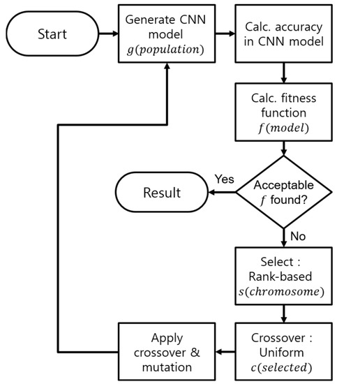
Figure 3. Block diagram explaining the process of our Genetic Algorithm (GA).

In order for any Genetic-type algorithm to optimise a given task, it first requires mapping of the solution into the search space of the algorithm. The key to the mapping process is to find a suitable representation scheme, so that solutions can be successfully described as chromosomes-sequences of genes. Genes can be represented by binary digits, alphabets, or floating point numbers.

For our algorithm, we use binary representation to encode connections between convolutional layers. An example of encoding such a connection is shown in Figure 4. We define a set of convolutional layers—layers that are in between input and pooling layers; two pooling layers; or pooling and fully connected layers—as a stage. For each layer within a stage, we call it a node. The structure shown in Figure 4 has one stage, with three nodes within the stage. We then convert the connection between each node into binary numbers. Only forward connections are allowed, and preceding connections of each node are encoded. Finally, stages are separated with bars, and nodes are separated with hyphens. The number of bits required to encode a network with S stages, where each stage has $K_S$ nodes, and is calculated with (5).

$$\begin{array}{c}\hfill numberofbits=\sum _S\frac{1}{2}{K}_S(K_S-1)\end{array}$$

(5)

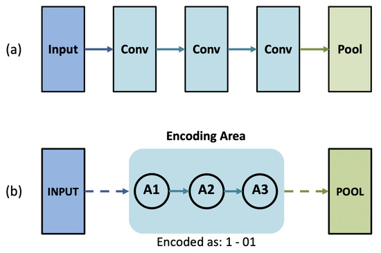
Figure 4. Encoding stages of architectures into binary strings. (a)-set of convolutional layer; (b)-encoded version of the layers in (a). In (b), numbers before and after the hyphen represent connections to node $A2$ and $A3$, respectively.

We also encode activation functions and optimisation algorithms into bits, and separate them with bars. The number of bits required for n hyperparameters can be calculated using (6).

$$\begin{array}{c}\hfill numberofbits=\lfloor {log}_2\left(n\right)\rfloor +1\end{array}$$

(6)

Definition of the encoding procedure is very important for our process, as it is used from the start of the algorithm—initialization. This step generates a population of CNN models in encoded, binary form. This step generally uses information from a previous generation to generate models, but for the first generation, it initialises the process by randomly creating a number of candidates. Each of the population is called as a chromosome, s. During this process, each bit of a chromosome is sampled independently using a Bernoulli distribution.

With provided population of networks, the algorithm decodes each of them and calculates the classification accuracy. These accuracies are used as fitness scores for the algorithm. The fitness score is also considered as the objective function of the algorithm, as it decides the survival of each chromosome. In our algorithm, we set an optimal fitness score, and repeat the entire procedure until a CNN model achieves this score.

If none of the population achieved the optimal fitness score, our algorithm then selects number of chromosomes, using a rank-based system. In this system, chromosomes with higher classification accuracies will survive, which ensures fast convergence of the algorithm.

After selection stage, survived chromosomes create the next generation of individuals through a uniform crossover process, c. This process selects a random pair of parent chromosomes, and generates offspring using a random variable. If this variable is larger than a predefined threshold, parent 1’s gene is taken. Else, parent 2 is chosen.

Finally, mutation is applied to the surviviving chromosomes. This process changes each gene in the chromosome with some probability, increasing the search space of the problem. Mutation occurs in a fixed number of generations, and can occur on chromosomes that have been generated as a result of the crossover process.

As our algorithm uses classification accuracy as the measurement of fitness, the resulting network structure and hyperparameter selection depend significantly on the input dataset. In this paper, we test our algorithm using an 18F-Florbetaben Amyloid PET/CT image dataset, which is used to diagnose symptoms of AD.

3.2. Dataset

The PET/CT dataset used in this paper was sampled from 18F-Florbetaben Amyloid PET/CT images recorded by the Nuclear Medicine department in Dong-a University Hospital between November 2015 to February, 2019. The sampled dataset was then verified by the Neurology department in the same hospital, through clinical tests such as neurophysiological testing. We eliminated samples with different cases of dementia. The final dataset included brain images of 414 patients, who have been diagnosed as Normal Control (NC), Mild Cognitive Impairment (MCI), and AD. Images of each classes are shown in Figure 5.

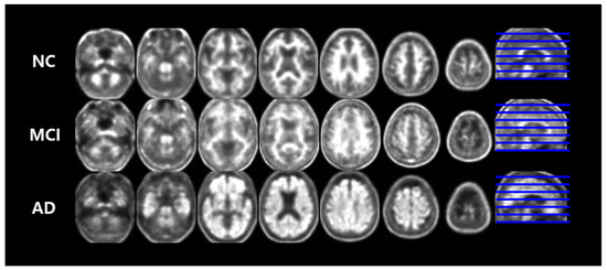
Figure 5. Multi-slices of pre-processed 18F-Florbetaben imaging by disease group. Each column shows 7 axial planes observed at equal intervals, and a sagittal plane. The blue lines represent the extracted level of each axial plane.

The original dataset, which is reconfigured from a PET camera, is a set of 3D images of size $400\times 400\times 110$. This image represents a section of brain with a thickness of $1.5$ mm. Each individual PET is non-linearly spatially transformed from the native PET image space to Montreal Neurological Institute (MNI) template space using an in-house PET template created from Dong-A University Hospital [29,30]. Each voxel count was then normalized to the whole cerebellar mean uptake to correct the image intensity due to differences in the amount of radioactive isotopes injected or individual characteristics. Specifically, all images were processed using Matlab2018a and SPM12 old_normalize modules beforebeing used as an input of the classifier.

After all sampling and processing, our dataset has a size of $95\times 79\times 68$. To use as the input for 2D Classification networks, 68 separate images from each patient were extracted and the images were resized to $100\times 100$. The dataset was divided into training and test sets with a ratio of 9:1. Stratified sampling was used to create these sets of data. Detailed information about this dataset is shown in Table 1.

Table 1. Details of the dataset.

Image Type	NII Images
Classes	Number of Subjects	Number of Images
	Train Set
AD	159	10,812
MCI	130	8840
NC	85	5780
	Test Set
AD	17	1156
MCI	14	952
NC	9	612

4. Results and Discussion

4.1. Experiment Settings

For the experiment, we created a neural network with $S=3$, with nodes $(K_1,K_2,K_3)=3,4,5$. Using the relevant equation from Genetic-CNN, we can calculate the number of bits that is required to encode the network.

$$\begin{array}{c}\hfill \sum _s\frac{1}{2}{K}_s(K_s-1)=3\left(2\right)+4\left(3\right)+5\left(4\right)=19\end{array}$$

(7)

In addition, we included two hyperparameters, activation function and optimisation algorithm, in the search space. Three activation functions, ReLU, Leaky ReLU, and Clipped ReLU, were used. We set $\alpha$ value of Leaky ReLU as $0.01$, and ceiling of Clipped ReLU as 10. Similarly, three optimisation algorithms were used; SGDM with a momentum value of $0.9$, RMSProp with $\beta =0.999$ and Adam with ${\beta }_1=0.9,{\beta }_2=0.999$. Each hyperparameter requires two extra bits when encoded, and the encoding rule is described in Table 2. Overall, the total length of the chromosome was 23.

Table 2. Encoding rule for hyperparameters.

Activation Function		Optimization Algorithm
Hyperparameter	Bit Representation	Hyperparameter	Bit Representation
ReLU	00	SGDM	00
Leaky ReLU	01	RMSProp	01
Clipped ReLU	11	Adam	11

The number of individuals, N, is set to 10, and the algorithm will repeat for 50 generations. For the evaluation process, each selected chromosome is decoded into the network architecture. Each of the decoded networks were trained for 50 epochs and tested to obtain the accuracy of the network. Accuracy values were then used as fitness value for the selection process.

4.2. Results

The results of the experiment are shown in Table 3. For each of the generations stated in the table, maximum, minimum and average accuracy of 10 individuals are shown. The best performing combination and network structure and hyperparameter set is also listed as encoded form.

Table 3. Results of the genetic algorithm, showing accuracy of generated networks.

Number of Generations	Accuracy (%)			Best Combination of Network Structure and Hyperparameters
	Maximum	Minimum	Average
0	46.45	40.89	43.61	0-11 | 1-01-111 | 1-01-110-1101 | 10 | 00
1	46.45	38.25	42.78	0-11 | 1-01-111 | 1-01-110-1101 | 10 | 00
2	47.81	44.89	46.68	0-11 | 1-10-111 | 1-01-110-1101 | 10 | 00
5	47.81	48.63	48.24	0-11 | 1-10-111 | 1-01-110-1101 | 10 | 00
10	64.64	58.49	61.56	1-01 | 1-10-111 | 1-01-110-1101 | 01 | 01
20	71.48	67.86	69.67	1-01 | 0-11-010 | 1-01-101-1101 | 10 | 00
50	82.64	80.84	81.74	1-11 | 1-10-111 | 1-11-011-0111 | 10 | 10

Figure 6 visualises the accuracy values for each generation in graph form. Convergence of three accuracy values is observed, showing that all individuals in the algorithm found the ideal neural architecture as the number of generations increases.

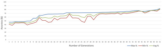
Figure 6. Graph showing the accuracy of networks against the number of generations.

To evaluate the performance of our algorithm with other state-of-the-art GAs, we ran the original Genetic-CNN with the same input dataset, and compared the average accuracy of individuals for different numbers of generations. This algorithm uses ReLU and Adam as hyperparameters to calculate their fitness values. The result is shown in Table 4. In early generations, individuals in the Genetic-CNN algorithm seem to learn faster. However, after the final generation, our algorithm found a neural architecture, including set of hyperparameters, that had $11.73\%$ higher classification accuracy for given input data.

Table 4. Comparison of our algorithm with Genetic CNN [7].

Number of Generations	Average Accuracy (%)		Difference (%)
	Genetic CNN [7]	Ours
0	23.29	43.61	20.32
1	23.29	42.78	19.49
2	28.95	46.68	17.73
5	51.91	48.24	−3.67
10	58.51	61.56	3.05
20	63.61	69.67	6.06
50	70.01	81.74	11.73

Our algorithm has four further bits compared with Genetic-CNN, due to the larger search space. However, the increase in processing time is minimal. The processing times required to obtain the result shown in Table 4 for Genetic-CNN and our algorithm were 618,278 s and 619,784 s, respectively. Only an increase of $0.24\%$ was observed, which is negligible.

The final network architecture is visualised in Figure 7. The first stage of the network is a residual architecture that is used in ResNet. The next stage has a multiple-path network similar to GoogLeNet, as outputs of three previous layers are used as input of other convolutional layers. The final stage has a highway-style structure, but not as complex as DenseNet. In addition, this network uses Clipped ReLU and Adam as their activation function and optimisation algorithm, respectively.

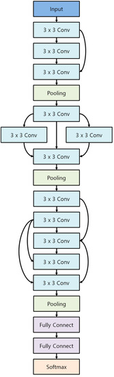
Figure 7. Final network architecture suggested by GA.

We also compared the network architecture from our genetic process to other state-of-the-art classification networks. Table 5 lists the accuracy of each network. The number of weighted layers in each network is also listed because this is related to the computational complexity of the network. Deeper networks typically have a better classification accuracy for any input dataset, but with the cost of computational complexity. An ideal deep learning network should perform well (high accuracy) and have a small number of layers.

Table 5. Comparison of our network with state-of-the-art networks.

Network	Number of Layers	Accuracy (%)
AlexNet [31]	8	55.83
VGG-16 [10]	16	57.79
SqueezeNet [32]	18	68.37
Autoencoder [33]	-	69.63
GoogLeNet [12]	22	70.45
ResNet50 [11]	50	85.20
Ours	14	81.74

From the table, we can see that the performance of our network is better than all other state-of-the-art networks, except for ResNet-50, with 50 weighted layers. However, the number of layers in our network is significantly lower than that of ResNet (more than $3\times$ lower). In addition, as the performance of the network with similar number of layers, VGG 16, is much worse than ours, it is possible to deduce that our network is extremely powerful.

5. Conclusions

In this paper, the aim was to optimise the configuration of CNN models for a given input dataset, using our algorithm. With 18F-Florbetaben Amyloid PET/CT images, architectures from our algorithm achieved an average classification accuracy of $81.74\%$, with a network consisting of only 14 weighted layers. In addition, we observed that accuracy values (minimum, maximum and accuracy) converged as the generation progressed. This proves that our algorithm is able to find the optimum set of network structure and hyperparameters, and is significantly better than other genetic algorithms.

In future, we aim to adapt our genetic algorithm to include various input datasets, as each input will create a different error surface for the classification task. Moreover, it would be ideal to include a further selection of hyperparameters.

References

- Roychaudhuri, R.; Yang, M.; Hoshi, M.M.; Teplow, D.B. Amyloid β-Protein Assembly and Alzheimer Disease. J. Biol. Chem. 2009, 284, 4749–4753. [Google Scholar] [CrossRef] [PubMed]
- Yoder, K.K. Basic PET Data Analysis Techniques. In Positron Emission Tomography-Recent Developments in Instrumentation, Research and Clinical Oncological Practice; IntechOpen: London, UK, 2013. [Google Scholar] [CrossRef]
- Higaki, A.; Uetani, T.; Ikeda, S.; Yamaguchi, O. Co-authorship network analysis in cardiovascular research utilizing machine learning (2009–2019). Int. J. Med. Inform. 2020, 143, 104274. [Google Scholar] [CrossRef] [PubMed]
- Myszczynska, M.A.; Ojamies, P.N.; Lacoste, A.M.B.; Neil, D.; Saffari, A.; Mead, R.; Hautbergue, G.M.; Holbrook, J.D.; Ferraiuolo, L. Applications of machine learning to diagnosis and treatment of neurodegenerative diseases. Nat. Rev. Neurol. 2020, 16, 440–456. [Google Scholar] [CrossRef] [PubMed]
- Zoph, B.; Vasudevan, V.; Shlens, J.; Le, Q.V. Learning Transferable Architectures for Scalable Image Recognition. In Proceedings of the 2018 IEEE/CVF Conference on Computer Vision and Pattern Recognition, Salt Lake City, UT, USA, 18–22 June 2018; pp. 8697–8710. [Google Scholar]
- Zhi, H.; Liu, S. Face recognition based on genetic algorithm. J. Vis. Commun. Image Represent. 2019, 58, 495–502. [Google Scholar] [CrossRef]
- Xie, L.; Yuille, A. Genetic CNN. In Proceedings of the 2017 IEEE International Conference on Computer Vision (ICCV), Venice, Italy, 22–29 October 2017; pp. 1388–1397. [Google Scholar]
- LeCun, Y.; Boser, B.; Denker, J.S.; Henderson, D.; Howard, R.E.; Hubbard, W.; Jackel, L.D. Backpropagation Applied to Handwritten Zip Code Recognition. Neural Comput. 1989, 1, 541–551. [Google Scholar] [CrossRef]
- Curry, H.B. The method of steepest descent for non-linear minimization problems. Q. Appl. Math. 1944, 2, 258–261. [Google Scholar] [CrossRef]
- Simonyan, K.; Zisserman, A. Very Deep Convolutional Networks for Large-Scale Image Recognition. In Proceedings of the 3rd Int. Conf. Learn. Representat, San Diego, CA, USA, 7–9 May 2015. [Google Scholar]
- He, K.; Zhang, X.; Ren, S.; Sun, J. Deep Residual Learning for Image Recognition. In Proceedings of the 2016 IEEE Conference on Computer Vision and Pattern Recognition, Las Vegas, NV, USA, 27–30 June 2016; pp. 770–778. [Google Scholar]
- Szegedy, C.; Liu, W.; Jia, Y.; Sermanet, P.; Reed, S.; Anguelov, D.; Erhan, D.; Vanhoucke, V.; Rabinovich, A. Going deeper with convolutions. In Proceedings of the 2015 IEEE Conference on Computer Vision and Pattern Recognition, Boston, MA, USA, 7–12 June 2015; pp. 1–9. [Google Scholar]
- Srivastava, R.K.; Greff, K.; Schmidhuber, J. Training Very Deep Networks. In Advances in Neural Information Processing Systems 28; Curran Associates, Inc.: Montreal, QC, Canada, 7–10 December 2015; pp. 2377–2385. [Google Scholar]
- Huang, G.; Liu, Z.; Van Der Maaten, L.; Weinberger, K.Q. Densely Connected Convolutional Networks. In Proceedings of the 2017 IEEE Conference on Computer Vision and Pattern Recognition (CVPR), Honolulu, HI, USA, 22–25 July 2017; pp. 2261–2269. [Google Scholar]
- Mohandes, M.; Codrington, C.W.; Gelfand, S.B. Two adaptive stepsize rules for gradient descent and their application to the training of feedforward artificial neural networks. In Proceedings of the 1994 IEEE International Conference on Neural Networks, Orlando, FL, USA, 28 June–2 July 1994; Volume 1, pp. 555–560. [Google Scholar]
- Weir, M.K. A method for self-determination of adaptive learning rates in back propagation. Neural Netw. 1991, 4, 371–379. [Google Scholar] [CrossRef]
- Nair, V.; Hinton, G.E. Rectified Linear Units Improve Restricted Boltzmann Machines. In Proceedings of the 27th International Conference on Machine Learning, Haifa, Israel, 21–24 June 2010; pp. 807–814. [Google Scholar]
- Maas, A.L.; Hannun, A.Y.; Ng, A.Y. Rectifier Nonlinearities Improve Neural Network Acoustic Models. In Proceedings of the 30th Int. Conf. Mach. Learn, Atlanta, GA, USA, 17–19 June 2013. [Google Scholar]
- Hannun, A.Y.; Case, C.; Casper, J.; Catanzaro, B.; Diamos, G.; Elsen, E.; Prenger, R.; Satheesh, S.; Sengupta, S.; Coates, A.; et al. Deep Speech: Scaling up end-to-end speech recognition. arXiv 2014, arXiv:abs/1412.5567. [Google Scholar]
- Bottou, L. Online Learning and Stochastic Approximations. In On-Line Learning in Neural Networks; Publications of the Newton Institute, Cambridge University Press: Cambridge, UK, 1999; pp. 9–42. [Google Scholar]
- Qian, N. On the momentum term in gradient descent learning algorithms. Neural Netw. 1999, 12, 145–151. [Google Scholar] [CrossRef]
- Tieleman, T.; Hinton, G. Lecture 6.5—RmsProp: Divide the gradient by a running average of its recent magnitude. In COURSERA: Neural Networks for Machine Learning; COURSERA: San Diego, CA, USA, 2012. [Google Scholar]
- Kingma, D.P.; Ba, J. Adam: A Method for Stochastic Optimization. In Proceedings of the 3rd Int. Conf. Learn. Representat, San Diego, CA, USA, 7–9 May 2015. [Google Scholar]
- Elsken, T.; Metzen, J.H.; Hutter, F. Neural Architecture Search: A Survey. J. Mach. Learn. Res. 2019, 20, 1–21. [Google Scholar]
- Zoph, B.; Le, Q.V. Neural Architecture Search with Reinforcement Learning. arXiv 2017, arXiv:cs.LG/1611.01578. [Google Scholar]
- Liu, H.; Simonyan, K.; Yang, Y. DARTS: Differentiable Architecture Search. arXiv 2019, arXiv:cs.LG/1806.09055. [Google Scholar]
- Elsken, T.; Metzen, J.H.; Hutter, F. Simple And Efficient Architecture Search for Convolutional Neural Networks. arXiv 2017, arXiv:stat.ML/1711.04528. [Google Scholar]
- Kandasamy, K.; Neiswanger, W.; Schneider, J.; Poczos, B.; Xing, E.P. Neural Architecture Search with Bayesian Optimisation and Optimal Transport. In Proceedings of the 32nd International Conference on Neural Information Processing Systems, Montreal, QC, Canada, 3–8 December 2018; pp. 2020–2029. [Google Scholar]
- Kang, H.; Kim, W.G.; Yang, G.S.; Kim, H.W.; Jeong, J.E.; Yoon, H.J.; Cho, K.; Jeong, Y.J.; Kang, D.Y. VGG-based BAPL Score Classification of 18F-Florbetaben Amyloid Brain PET. Biomed. Sci. Lett. 2018, 24, 418–425. [Google Scholar] [CrossRef]
- Kang, H.; Park, J.S.; Cho, K.; Kang, D.Y. Visual and Quantitative Evaluation of Amyloid Brain PET Image Synthesis with Generative Adversarial Network. Appl. Sci. 2020, 10, 2628. [Google Scholar] [CrossRef]
- Krizhevsky, A.; Sutskever, I.; Hinton, G.E. ImageNet Classification with Deep Convolutional Neural Networks. Adv. Neural Inf. Process. Syst. 2012, 25, 1106–1114. [Google Scholar] [CrossRef]
- Iandola, F.N.; Han, S.; Moskewicz, M.W.; Ashraf, K.; Dally, W.J.; Keutzer, K. SqueezeNet: AlexNet-level accuracy with 50× fewer parameters and <0.5 MB model size. arXiv 2016, arXiv:cs.CV/1602.07360. [Google Scholar]
- Goodfellow, I.; Bengio, Y.; Courville, A. Autoencoders. In Deep Learning; MIT Press: Cambridge, MA, USA, 2016. [Google Scholar]
Publisher’s Note: MDPI stays neutral with regard to jurisdictional claims in published maps and institutional affiliations. |
© 2021 by the authors. Licensee MDPI, Basel, Switzerland. This article is an open access article distributed under the terms and conditions of the Creative Commons Attribution (CC BY) license (http://creativecommons.org/licenses/by/4.0/).