Finite Element Models of a Benchmark Footbridge

Abstract

Modern footbridges are often lively structures, characterized by natural frequencies that fall in the range of pedestrian activities, such as walking, running, and jumping. Therefore, serviceability assessment under human-induced excitation is crucial both at the design stage and during the footbridge lifetime. This paper presents and validates two different FE models of an existing footbridge with very complex geometry: the Streicker Footbridge at the Princeton University Campus. It represents a benchmark in the field as a testbed for vibration serviceability assessments under pedestrian excitation. The real structure is equipped with strain and temperature sensors that are currently used to collect measurements in both static and dynamic modes for research and educational purposes in Structural Health Monitoring (SHM). Based on detailed drawings of the Streicker Footbridge, a three-dimensional beam-based model was developed to represent the complex behavior of the full-scale benchmark bridge. Subsequently, a more refined discretization of the bridge deck adopting shell elements was inserted. The bridge Finite Element models were validated against available SHM data concerning static and dynamic tests. The relevant ANSYS APDL script files along with an example of pedestrian jumping application are available upon request for further research developments on the relationship between pedestrians and the benchmark footbridge.

1. Introduction

Serviceability assessment of footbridges under human-induced excitation has become a challenging engineering problem since the London Millennium Bridge was closed in 2000 due to unexpected lateral vibrations induced by synchronized pedestrians [1]. That episode highlighted a gap in the knowledge and related code provisions concerning pedestrian dynamic loads and their dynamic effect on flexible structures. Since then, a great number of studies have been devoted to fill the gap, and significant advancements have been made both in the phenomenological analysis and in the modelling of dynamic loads induced by walking pedestrians (for a review see, e.g., [2,3,4]). Despite this, there is still lack of an unanimously accepted procedure to assess the dynamic behavior of footbridges under pedestrian excitation.

In this context, the current knowledge could be greatly extended by making available experimental data collected on real footbridges, which so far are very scarce. Actually, despite several papers have been published on case studies of existing footbridges (e.g., [5,6,7,8]), experimental data were rarely made available to the scientific community. To the authors’ best knowledge, only three examples exist in the literature. The first one is the benchmark footbridge described by Zivanovic [9], i.e., the Podgorica footbridge in Montenegro. Collected data concern both the dynamic response measured under operating traffic conditions and statistics of the pedestrians’ speed and frequency, as well as the footbridge mode shape. The second dataset is the one collected by Gomez et al. [10] on a 12 m-long laboratory footbridge, specifically built as a testbed to study human–structure interaction. The footbridge dynamic response was recorded during one people crossing: 100 people crossed the footbridge 20 times each at frequencies controlled through a metronome. Pedestrian crossings were recorded through a videocamera in order to correlate the pedestrian kinematics to the footbridge dynamic response. The third dataset was collected by Van den Broeck et al. [11] on the Eeklo footbridge. It consists of four data blocks involving two pedestrian densities, 0.25 ped/m${}^2$ and 0.50 ped/m${}^2$, representing a total of more than one hour of data for each pedestrian density: footbridge response and pedestrian trajectories were simultaneously recorded. All these examples are characterized by quite simple footbridge structures and by unrestricted pedestrian traffic, i.e., with very low pedestrian densities. Moreover, detailed data on footbridge structures, useful for building Finite Element Models, are not always available.

The aim of this paper is to make available to the scientific community a new benchmark structure, the Streicker footbridge, which is in service at the Princeton University Campus. The Streicker footbridge overpasses a busy roadway, but is used also for research and educational purposes related to Structural Health Monitoring (SHM) (e.g., [12,13,14,15]). With respect to the previously cited benchmarks, the Streicker bridge is characterized by a complex geometry. In plan view, two coupled arches form an X-shape, developing a considerable deck stiffness in the lateral direction. In the vertical plane, a series of metallic supports, i.e., a central arch and a series of lateral piers under the approach legs, bear vertical loads. The dynamic properties of the Streicker footbridge make it particularly responsive to excitation frequencies typical of pedestrians’ running conditions. Hence, the Streicker footbridge is particularly suitable as a benchmark structure to investigate the dynamic effects of running pedestrians. Actually, despite a great number of studies that were devoted in the last two decades to characterize and model the walking excitation (for a review, see, e.g., [16]), the running excitation has been far less studied [17,18,19].

Furthermore, the Streicker footbridge embeds a complex monitoring system with a number of sensors that have already been used in several research studies. The aim of transforming the Streicker bridge into an on-site laboratory for various research and educational purposes is presented in [12]. The real-time detection and characterization of early-age thermal cracks in the concrete deck is presented in [13], along with details on the discrete and distributed fiber optic sensors arrangement. A universal method for the determination of the distribution of prestressing forces along the concrete deck of the Streicker Bridge is developed in [14,15] using the embedded long-gauge fiber optic sensors. The Streicker Bridge was also used in [20] to test a newly designed stand-alone sensor equipped with an MEMS-based accelerometer and a wireless transmission unit for vibration monitoring. Recent developments [21,22] presented the modal frequencies identification of the Streicker Bridge by output-only approaches. Furthermore, these last studies proposed to develop a wireless network monitoring system to be applied in parallel to the embedded fiber optic system for a comprehensive assessment of the stiffer component (the main span) of the bridge, where only minor strains are registered by the fiber optic sensors.

Although a significant amount of expertise was accumulated in the described research literature, little knowledge was gained on the effects of the pedestrian loads on the Streicker Bridge. In particular, the structure can be subjected to amplification in the typical frequencies of pedestrian running over the main span and the south-east approaching leg. Furthermore, the effects of running individuals may amplify the bridge response with respect to local modes, owing to the peculiar characteristics of the structure. In this perspective, different vibration control solutions, such as TMDs or linear dampers, can be designed and evaluated according to different schemes, e.g., hybrid solutions, decentralized and semi-active [23,24,25,26,27,28].

This paper presents a new phase of the research on the Streicker Bridge benchmark. The general aim is the derivation of refined FE models of the structure with different levels of accuracy for serviceability assessment under pedestrian loading, structural control and SHM purposes. The presented FE models, developed in ANSYS APDL [29], are validated against available static and dynamic experimental data collected by the embedded monitoring system on the footbridge, namely static displacements, moment influence lines and modal responses. The paper is completed by an example of pedestrian jumping load applied to the more refined FE model. The source files of the developed FE models will be made available to researchers who are interested in carrying out studies on the above-mentioned topics. In particular, possible applications of the developed FE models are the investigation of pedestrian interaction with the system dynamics, the proposal and testing of new models of running excitation, the design of vibration response mitigation measures, damage detection or model updating.

The paper develops as follows: Section 2 focuses on the presentation of the Streicker Footbridge, while the subsequent Section 3 and Section 4 are devoted to the presentation of the FE model development and their validation. Section 5 presents the pedestrian loading application, while concluding remarks are outlined in Section 6.

2. Description of the Benchmark Footbridge

2.1. Footbridge Layout

The Streicker footbridge, 104 m long, is located at the Princeton University (PU) Campus (Princeton, NJ, USA) and connects the western to the eastern part of the campus [12]. It consists of a main span, (deck stiffened arch) and four lateral approaching legs (continuous curved girders), see Figure 1. Conceptual design of the bridge was made by Christian Menn, details were developed by Theodore Zoli and Ryan Woodward of HNTB Corporation, while the construction was performed by the Turner Construction Company under leadership of Steve Hancock. In plan, the footbridge geometry results from two intersecting arches that assure lateral stability to the steel arch supporting the main span.

The deck, made of post-tensioned high-performance concrete, is connected through six spandrels (Figure 2 right) to the steel arch in the main span and is supported by eight Y-shaped piers along the lateral legs (Figure 2 left). The main arch, spandrels and piers are made of weathering steel tubes filled with self-consolidating concrete. The diameter of the tubular arch beams is 324 mm. The deck cross-section width is equal to 3.04 m in the four legs, and variable in the main span, with a maximum width of about 7.4 m in the sections where the legs join the main span. The depth of the deck is variable as well, and equals 578 mm in the legs. At the abutments, the deck rests on elastomeric neoprene bearings (Figure 3 left). Both piers and arch are fixed to concrete footings, which are supported on micropiles (Figure 3 right). The deck is connected to the piers and spandrels through bolted connections.

2.2. Materials

The concrete mixture for the deck was designed according to the New Jersey Department of Transportation (NJDOT) specifications for Class A High-Performance Concrete (HPC) [30]. The average 28-day compressive strength from cylinder tests was 51 and 59 MPa for the main span and the legs, respectively [12]. The Young’s modulus was 37.5 GPa [31]. The arch, piers and spandrels are made of round hollow structural steel (HSS) with a minimum yield strength of 345 MPa and a minimum ultimate strength of 483 MPa, in conformity to ASTM A847-05. All the pipes are designated as CFT (concrete filled tubes) with Yoloy weathering steel type.

2.3. Design Loads

The dead loads adopted in the design are listed in

Table 1. Design dead loads.

Reinforced concrete [kN/m${}^3$]	23.56
Post-tensioned concrete [kN/m${}^3$]	24.35
Structural steel [kN/m${}^3$]	76.97
Bridge railings [kN/m]	0.730
Utilities [kN/m]	0.219
Future wearing surface [kN/m${}^2$]	0.718

. The pedestrian live load, defined according to AASHTO (Guide Specifications for Design of Pedestrian Bridges, Section 1.2), is equal to 31.11 kN/m${}^2$ [32]. The design wind loads are equal to 3.59 kN/m${}^2$, applied on the vertical projected area perpendicular to the longitudinal axis.

2.4. Monitoring Systems

During construction, the Streicker bridge was equipped with two fiber optic-based monitoring systems embedded in the concrete deck [12] with the aim of transforming the bridge into an on-site laboratory for research and educational purposes. The system was conceived for global structural monitoring based on discrete fiber Bragg-grating (FBG), long-gauge strain and temperature sensors and a Brillouin-scattering based distributed sensing system used for integrity monitoring. Since the bridge is almost doubly symmetrical in plan, the sensors were installed on half the main span and on the south-east leg, which is the longest one (Figure 4). Only the FBG system is relevant for this research work due to its capability for dynamic monitoring. In particular, measurements from parallel sensors are taken into account in this study. These sensors are installed in couples parallel to the center line of the deck close to the axis of symmetry of each cross-section, one sensor at the top and one at the bottom. This allows for curvature calculations based on the strain measured at the top and bottom sensors. The specifications of the SHM system can be summarized as follows: resolution 1.7 $\mathsf{\mu }\mathsf{ϵ}$, repeatability <1 $\mathsf{\mu }\mathsf{ϵ}$, typical gauge length 60 cm (30–120 cm), dynamic range from −5000 to 7500 $\mathsf{\mu }\mathsf{ϵ}$ and maximum measurement frequency 250 Hz [31].

2.5. Field Tests

Field tests were performed to study the footbridge performances under both static and dynamic loads.

Static tests were performed in March 2011 by using four golf carts of 4.5 kN each as a moving static load [31]. Two carts were positioned side by side across the bridge width at 13 different locations along the instrumented length of the footbridge. Moment influence lines were obtained by calculating the curvature at each sensor location and by multiplying it by the flexural stiffness $EI$ of the cross-section. Another static test was performed in April 2014 by positioning an approximately four-metric-ton truck (about 46.7 kN) in the middle of the longest span of the bridge, i.e., between P10 and P11 on the south-east leg [33]. The rear axle, which introduced the greatest portion of the load (42 kN), was placed directly above the sensors in the middle of the longest span. Displacements were obtained by double integration of the curvature, measured by sensors. Moreover, an independent displacement measurement using a laser was performed by a research group from Columbia University.

The footbridge natural frequencies were obtained through different dynamic tests (

Table 2. Summary of identified natural frequencies [Hz].

Ref.	${\mathit{f}}_{\mathbf{1}}$	${\mathit{f}}_{\mathbf{2}}$	${\mathit{f}}_{\mathbf{3}}$	${\mathit{f}}_{\mathbf{4}}$	${\mathit{f}}_{\mathbf{5}}$	${\mathit{f}}_{\mathbf{6}}$
Sigurdardottir and Glisic [12,31]	3.11–3.17	3.72
Sabato [20]	3.08	3.75
Domaneschi et al. [22]	3.00	3.65	4.46	4.95	6.02	7.81
Brown et al. [34]	3.00

). The ones described in [31] were performed in 2010 and refer to synchronized people running at 3 Hz, 4 Hz and at random frequencies for 30 s. Natural frequencies were extracted from Fast Fourier Transform (FFT) of the strain sensor measurements at the midspan between piers P10 and P11. From the tests with excitations of 3 and 4 Hz, two frequencies were identified, at 3.11 and 3.72 Hz, respectively. These values were confirmed by the test with random excitation (3.17 and 3.72 Hz). A subsequent measurement campaign was performed in 2014 with similar tests. Data were analyzed in [22], identifying the first two natural frequencies at around 3 and 3.6 Hz. Moreover, natural frequencies of higher modes (from third to sixth) were also identified. Sabato [20] performed quasi-static and dynamic tests by installing a newly designed wireless system (Acceleration Evaluator, ALE), which embeds an MEMS-based accelerometer. The ALE transmitter was installed at one-quarter of the south-east leg length, starting from the connection with the main span. Dynamic tests were performed with eight people jumping for 30 s at 3 Hz at the transmitter location and eight people running at random frequencies for 2 min between the main span–leg connection point and half of the leg total length. Identified frequencies were 3.08 and 3.75 Hz. Finally, Brown et al. [34] tested an alternative methodology to measure dynamic displacements based on digital videos. The bridge deck was excited by people jumping on the south-east leg. Postprocessing of recorded videos allowed us to extract the vertical displacement response and to identify two peaks at 3 and 6.3 Hz, respectively.

The small magnitude load induced by people during the above tests produced small strain amplitudes that could be used to identify natural frequencies, but not to accurately find deformed and mode shapes. Nevertheless, it is worth recalling that, due to the parallel sensors position, only vertical flexural modes of the south-east leg can be detected.

3. Finite Element Models

Two different FE models were built in ANSYS Mechanical APDL. The models are characterized by different levels of accuracy in describing the peculiar deck geometry, with a main span “splitting” in two legs at each side, which raises the problem of modelling the zones of transition between the central span and the legs. The first model, Beam (B model), contains only beam elements: the transition zone is approximately taken into account by creating a rigid region that connects the eccentric axis lines of central span and legs. In the second model, Shell (S model), the deck geometry in the plan is modelled with shell elements.

The two models, able to correctly describe the footbridge global structural behavior at different refinement levels, could be used for different purposes. For example, the S model, with its accurate description of the deck geometry in plan, allows us to perform numerical simulations of pedestrian traffic along any trajectory. Conversely, the B model provides a slender analysis tool when detailed spatial behavior of deck is not the focus of the analysis. In the following section, the two models share a set of assumptions and input data.

3.1. Modelling Assumptions

Both long-term effects on the concrete and the effect of the deck post-tensioning on the modal results were neglected, under the assumption of linear behavior of materials and perfect bond with tendons, since the variations in the deformed equilibrium configuration do not significantly modify the dynamic properties of the structure [35].

The real variable cross-sections of the deck, made complex by the interior holes (see Figure 2), were simplified through the definition of five equivalent rectangular sections, whose tensor of moments of inertia were provided as input in Ansys. The dimensions b and h of the equivalent cross sections are chosen to match the moments of inertia of the real cross section ($I_x=b{h}^3/12$, $I_y=h{b}^3/12$). The effective area ($A_{\mathrm{eff}}=bh$) of the equivalent sections is larger than the real one ($A_{\mathrm{real}}$), due to the presence of the holes.

Table 3. Equivalent rectangular cross-sections of the concrete deck [36].

	P6–P7	P5–P8	P4–P9	P3–P10	Legs
h (m)	0.523	0.5349	0.5484	0.56	0.4826
b (m)	3.68	4.15	5.05	6.70	3.20
$A_{\mathrm{eff}}$ (m${}^2$)	1.93	2.22	2.77	3.75	1.54
$A_{\mathrm{real}}$ (m${}^2$)	1.46	1.74	2.24	3.21	1.28
$I_x$ (m${}^4$)	0.04	0.05	0.07	0.10	0.03
$I_y$ (m${}^4$)	2.17	3.20	5.90	14.02	1.31

shows the dimensions of the equivalent sections, referring to the pier names (from pier P3 to pier P10) shown in the elevation view (Figure 1).

The elements of the arch, spandrels and piers are assigned tubular steel cross sections.

Table 4. Tubular steel cross sections of arch, spandrels and piers [36].

	Arch	Pier	Y-Shaped Pier	Spandrel
$r_1$ (m)	0.143	0.122	0.1	0.074
$r_2$ (m)	0.160	0.135	0.11	0.085
$A_s$ (m${}^2$)	0.017	0.01	0.007	0.005
$A_c$ (m${}^2$)	0.064	0.047	0.031	0.017

summarizes the dimensions of the assigned cross sections, where $r_1$ and $r_2$ are the internal and external radius, respectively.

Due to the difference in the effective area of the deck cross-sections, a reduction in the density of the concrete was applied in order to preserve the total mass.

Table 5. Concrete properties [36].

	P6–P7	P5–P8	P4–P9	P3–P10	Legs
${\rho }_{\mathrm{eff}}$ (kg/m${}^3$)	2070	2129	2173	2280	2269
$E_c$ (GPa)	35	35	35	35	36
$f_c$ (MPa)	41.37	41.37	41.37	41.37	41

reports the implemented concrete properties. Note that the value of ${\rho }_{\mathrm{eff}}$ also accounts for the additional contribution due to the railings, the utilities and the wearing surface. Similarly, the density of structural steel was modified to account for the concrete infilling (

Table 6. Steel properties [36].

	Arch	Pier (Base Column)	Pier (V-Pipes)	Spandrel
${\rho }_{\mathrm{eff}}$ (kg/m${}^3$)	14,915	16,281	16,336.6	13,616.6
$E_s$ (GPa)	206.87	210.64	213.04	200.36
$f_y$ (MPa)	344.74	344.74	344.74	344.74

).

In both models, the deck and the pier nodes at every pier/spandrel location are connected using rigid body constraints between the centroid of the deck and the two upper nodes of every Y-shaped pier or spandrel (three nodes in total). Thus, all degrees of freedom (six DOFs) are constrained, in accordance with the bolted connection between deck and pipes.

3.2. B Model

The B model was first developed in [36] and contains 98 nodes and 84 Timoshenko beam elements (Figure 5), named BEAM188, with six DOFs per node. This beam element can be used for both slender and stout beams. The deck elements were assigned the five equivalent rectangular cross-sections described in Table 3, depending on their position. Beam nodes do not have offset with respect to the mesh nodes that are located in the middle plane of the deck. In a similar way, the arch, piers and spandrels were modelled with four different pipe cross-sections based on their real dimensions (Table 4).

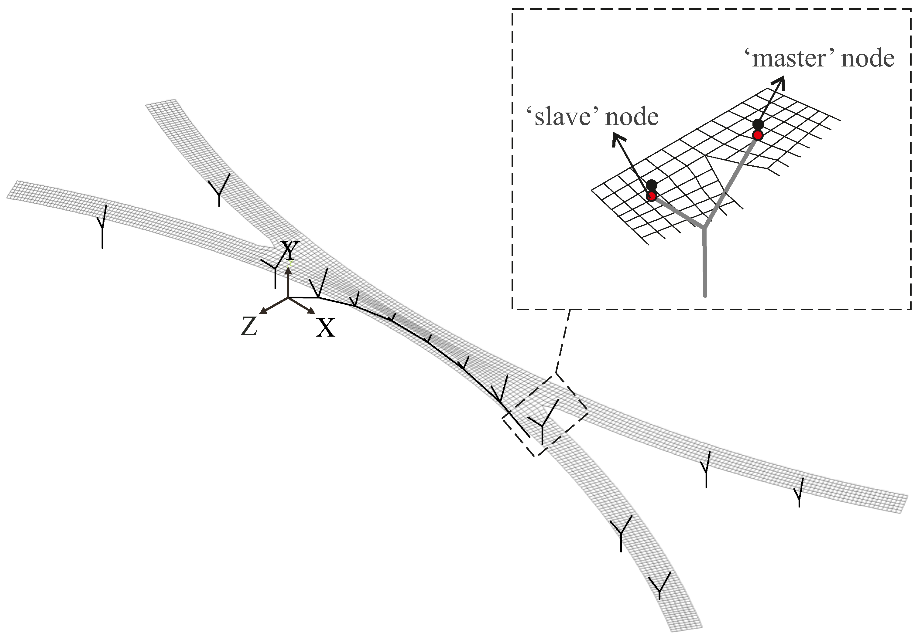
As can be noticed in Figure 5, the deck and pier nodes are not connected by beam elements, but by rigid links that constrain the six degrees of freedom of a removed (“slave”) node to the ones of a retained (“master”) node. For the case at study, the retained node is the deck node at the pier or spandrel locations and the removed nodes are the two upper nodes of every Y-shaped pier and spandrel. The six degrees of freedom of the removed nodes are all constrained in this way, and no independent equilibrium equation is written for them. The bases of the piers and of the arch are fixed, while the boundary conditions at the four abutments are 3D hinges. The model was preliminary validated by comparing the results of the vertical reactions due to self-weight (6902.50 kN) to the weight value computed manually (6904.72 kN).

3.3. S Model

A first version of the S model was developed in [36]. The improved S model, depicted in Figure 6, contains 3425 nodes. Furthermore, in this model, the BEAM188 element was used for the arch, piers and spandrels. The deck is discretized with SHELL181 elements, a four-node element with six DOFs at each node. This shell element is suitable for analyzing thin to moderately thick shell structures. In total, the S model contains 2995 elements: 43 beam elements to model the arch, piers and spandrels and 2952 shell elements to model the deck.

The shell elements adopted for the deck are quadrilateral, with an average size of approximately 0.5 × 0.5 m. The element nodes are created by a direct user-defined generation. Since the shell elements allow constructing a tapered deck, the variation of the cross-section in the main span of this model is smoother than in the B model. Adjacent shell elements connect to each other at the midplane of the deck, so they do not have an offset.

In the same way as for the B model, the arch, piers and spandrels adopt four different pipe cross-sections based on the real dimensions of the bridge. Differently from the B model, the deck is continuous between the legs and the main span. Similarly to the B model, the two upper nodes of the pier or spandrel are constrained to their closest node of the deck shell. The boundary conditions are the same as in the B model. The self-weight validation was also positively performed in this case.

4. Validation of FE Models

In this section, the two FE models are validated against experimental data collected during the static and dynamic tests briefly described in Section 2.5.

4.1. Static Analysis

The two static on-site tests (moving golf carts and static trucks) described in Section 2.5 are numerically simulated through the two FE models. In order to obtain moment influence lines to be compared with those experimentally measured, a resultant load of 18 kN, representing the total weight of four golf carts, was applied at different positions along the footbridge length. The load was differently distributed depending on the type of FE model. In the B model, the moving static load is applied as a single force of 18 kN concentrated on a deck node. In the S model, two different load distributions were tested (Figure 7):

L1:

the total load has been applied as three forces of 6 kN each on three nodes of the generic cross section, in order to reproduce the equivalent load condition as in the B model;

L2:

the total load has been spread over a larger portion of the deck and applied as nine concentrated loads corresponding to the axes of the four golf carts.

Figure 8, Figure 9 and Figure 10 plot the obtained bending moment influence lines at three pier locations: P8, P10 and P11h12 (at half the span between P11 and P12), respectively. Numerical influence lines are compared with those obtained from sensor measurements [12], which are reported in red solid lines together with measurement errors in red dashed lines.

In detail, the B model and S model with L1 provide almost the same results for the influence lines as in P8 and P11h12 (Figure 8 and Figure 10) because of the equivalent way in which the applied load is modeled. The rough representation of the loading conditions in these cases causes a discrepancy of about 50% between numerical and experimental outcomes at the peak bending moment in P8. On the contrary, considering the P10 location (Figure 9), the results highlight a higher variability between the B model numerical outcomes and the S ones, even when the load is applied in the same way. This is mainly due to the description of the connection between the main span of the bridge deck and the east legs (Figure 1), which is more accurately reproduced by the introduction of the shell elements for main girder modelling. Indeed, the S model influence lines at P10 are closer to the experimental ones.

The S model with L2, with a more realistic description of the applied load, gives the best fit to the experimental results, with numerical influence lines generally falling inside the error limits of experimental measurements. Focusing on the influence lines at P10 (Figure 9), the experimental influence line is best approximated by the S-L2 model (relative error at the peak moment of about 26% with S-L2 against 110% with the B model). In this case, the more realistic description both of the deck geometry at the connection between the south-east leg and main span and of the transit loading conditions allows for the solving of the large discrepancy between experimental and B-bending moments when the load is applied between P10 and P11. The large discrepancy that still remains when the load is applied in P10 is expected, because at this location there is the connection between two structures (main span and leg) built at different times, so its physical continuity is not guaranteed.

The second static test consists of the application of a concentrated load of 42.7 kN at a half span between P10 and P11 on the south-east leg. The load is applied as a single concentrated nodal force in the B model and divided into two concentrated nodal loads in the S model along the same cross-section. The displacements obtained along the south-east leg are compared with those estimated in [33], through double integration of the curvature according to both rectangular and trapezoidal rules, and with that measured by a laser. Figure 11 shows that the numerical predictions obtained with both the B and S models shows an excellent agreement with experimental results, i.e., they fall within the error limits (see errorbars in Figure 11) due to the numerical integration and the mechanical strain measurement.

It must be noticed that the two proposed models have not undergone a formal model updating process. The available data from the literature (e.g., materials and geometry) have been used. The proposed models could be enhanced, e.g., by varying the Young’s modulus more gradually along both the main span and legs in order to obtain a better fitting to experimental measurements. Nevertheless, considering that such variation for new structures is usually considered unrealistic, the model S-L2, with constant assumptions for structural parameters, represents the best fit as it has the smallest overall discrepancy compared with measurements. In summary, the S-L2 model is able to better represent the footbridge’s overall static behavior with respect to the B model.

4.2. Modal Analysis

Table 7. Summary of first 11 natural frequencies from B and S models [Hz].

	B Model		S Model
Mode	Frequency	Qualitative Description	Frequency	Qualitative Description
1	3.0869	Flexural-torsional	3.1197	Flexural vertical
2	3.1568	Flexural vertical	3.1451	Flexural-torsional
3	3.5925	Flexural vertical	3.5351	Flexural vertical
4	3.708	Flexural vertical	3.7129	Flexural vertical
5	4.1319	Flexural vertical	4.143	Flexural vertical
6	4.488	Flexural vertical	4.4908	Flexural vertical
7	4.6273	Flexural lateral	5.2466	Flexural-torsional
8	5.3695	Flexural-torsional	5.858	Flexural lateral
9	5.9998	Flexural lateral (east legs)	6.0714	Flexural-torsional
10	6.0627	Flexural lateral	6.3452	Flexural-torsional
11	6.4939	Flexural vertical	6.5534	Flexural vertical

summarizes the first eleven natural frequencies extracted through modal analysis from B and S models, with a qualitative description of the dominant deflected shape based on visual inspection of the mode shapes.

The experimental modes are extracted with reference to the embedded fiber optic sensors at the south-east leg (discrete strain sensors collecting dynamic response between two fibers in the vertical plane at the top and the bottom of the deck center line). Consequently, flexural vertical modes of the south-east leg are exclusively detected by the SHM system. Therefore, in the following, focus is made on mode shapes with a prevailing vertical component, which are plotted in Figure 12 and Figure 13.

Table 8. MAC between B and S mode shapes.

		S Model
		1	2	3	4	5	6	7	8
B Model	1	0.062	0.9098	0.0128	0.0055	0.0121	0.0013	0.0591	0.0686
	2	0.9658	0.0322	0.0011	0.0038	0	0.0006	0.0084	0.0234
	3	0.0002	0.0138	0.9976	0.0346	0.0378	0.0006	0.0016	0.003
	4	0.0009	0.0312	0.0151	0.9783	0	0.0032	0.0049	0.0398
	5	0.0042	0.0131	0.0437	0.0086	0.9912	0.0044	0.006	0.0084
	6	0.0045	0.0003	0.0015	0.0119	0.0012	0.9911	0.002	0
	7	0.02	0.4102	0.0155	0.0012	0.158	0.0586	0.2993	0.1816
	8	0	0.0409	0	0.0398	0.0026	0.0072	0.9229	0.139

reports the Modal Assurance Criterion (MAC) values between B and S mode shapes, calculated for the vertical component of the first eight modes. It can be observed that MAC values are very close to unity for modes 3 to 6. Some modes are ordered differently in the B and S models, e.g., mode shapes 1 and 2 present close natural frequencies, and they are reversed in the B model with respect to the S model. This is confirmed by MAC values, which are above 0.9 when mode 1-B and mode 2-S are considered (and vice versa). MAC values also highlight a high correlation between mode 8-B and mode 7-S. In this case, there is no evidence of mode inversion, i.e., it is not possible to identify a similarity between mode 7-B and mode 8-S. For a better comparison, Figure 12 and Figure 13 plot the modes that have the same mode shape in both models on the same row.

The analysis of frequencies and mode shapes allows outlining the following observations:

• The B and S models provide consistent results in terms of modal properties;
• Modes 1 and 2 have very close natural frequencies, and in both models, the south-east leg has a significant vertical component. The comparison with experimental natural frequencies makes it difficult to definitely identify which of the two numerical modes corresponds to the experimental first mode;
• Mode 3 mainly involves the main span and the south-west and north-east leg. This explains why it was not detected by sensors;
• Mode 4 is flexural vertical and has a frequency very close to the second experimental one.

In conclusion, it can be stated that any of the first two numerical modes could both correspond to the first experimental mode, while the fourth numerical mode probably corresponds to the second experimental one.

Table 9. Comparison between experimental and numerical frequencies.

Ref.	${\mathit{f}}_{\mathbf{exp}}$ [Hz]	${\mathit{f}}_{\mathbf{B}}$ [Hz]	${\mathit{ϵ}}_{\mathbf{B}}$ [%]	${\mathit{f}}_{\mathbf{S}}$ [Hz]	${\mathit{ϵ}}_{\mathbf{S}}$ [%]
Sigurdardottir and Glisic [12,31]	3.11	3.0869	0.	3.1197	0.31
	3.17	3.1568	−0.42	3.1451	−0.95
	3.72	3.708	−0.32	3.7129	−0.19
Sabato [20]	3.08	3.0869	0.22	3.1197	1.29
	3.08	3.1568	2.49	3.1451	2.11
	3.75	3.708	−1.12	3.7129	−0.99
Domaneschi et al. [22]	3.00	3.0869	2.90	3.1197	3.99
	3.00	3.1568	5.22	3.1451	4.84
	3.65	3.708	1.59	3.7129	1.72

reports the comparison between numerical and experimental frequencies, showing an excellent agreement (percentage errors $ϵ$ below 5%).

5. Dynamic Response under Jumping Pedestrian Excitation

The proposed application described in this section aims at presenting an example of simulation of dynamic response under human-induced excitation. In addition, it could be intended as a tentative validation of the dynamic behavior of the footbridge against experimental measurements of the acceleration response due to jumping pedestrians. Among the few experimental tests reported in the literature, which usually refer to pedestrians running along the south-east leg (Section 2.5), the ones described by Sabato [20] are considered since they are described in more detail, and time histories of the vertical acceleration are provided. In particular, in the test analyzed here, eight pedestrians jump at 3 Hz at about one-quarter of the way along the south-east leg for 30 s.

A limited number of pedestrian load models are available in the literature (e.g., [37,38]). The pedestrian jumping load model proposed in ISO 10137 [39] has been adopted for the following application. The load exerted by one jumping pedestrian is modelled as a perfectly periodic half-sine function:

$$F\left(t\right)=\left\{\begin{array}{cc}\alpha Gsin\left(2\pi f\right)& 0\le t\le t_c\\ 0& t_c<t\le T\end{array}\right\},$$

(1)

where $\alpha =2.1-0.15f$ is the dynamic load factor of the first harmonic of the load, G is the pedestrian weight, assumed equal to 700 N as usually is usually performed in the literature (e.g., [9]), f is the excitation frequency, $T=1/f$ is the period and $t_c$ is the contact time, assumed equal to $T/2$. In order to account for the fact that it is very difficult for people to jump in phase with each other, even if they try to intentionally excite the bridge by jumping [40], a random phase shift is assigned among the eight pedestrian loads: specifically, pedestrians are assumed to start jumping with a time shift randomly assigned between 0 and 0.33 s (where 0.33 s is the step period). Moreover, the load amplitude is further reduced by 20% to take into account a lower correlation between pedestrians [39].

The eight forces are applied at eight nodes of the S model around the section at a quarter of the south-east leg span. A full transient analysis is performed in Ansys. Damping is modelled according to the Rayleigh formulation, with mass and stiffness coefficients equal to 0.164 and 0.000153, respectively, estimated to obtain the experimental value of damping ratio of 0.57% [21] on the first numerical mode, and on the mode corresponding to a cumulated participation, mass in the vertical direction of around 60%. Time step is set equal to 0.02 s.

Figure 14 plots the numerical time history of the vertical acceleration at a quarter of the south-east leg in comparison with the one measured by Sabato [20]. The numerical response is much more regular than the experimental one. Actually, the perfectly periodic force model is not able to capture the inter- and intra-subject variability [41,42] that characterize pedestrian excitation. Moreover, the applied force does not account for human–structure interaction and for the related damping effect induced by human bodies [42]. Because of these two factors, the numerical structural response overestimates the experimental one by about 12.5% (if the initial peak due to transient, at around 5 s, is neglected). The comparison between Power Spectral Density (PSD) functions of the experimental and numerical response is shown in Figure 15. In the experimental results, peaks at both the bridge frequency and at pedestrian frequency are detected. On the contrary, the numerical PSD is concentrated on one single peak at the excitation frequency.

It should be stressed that the present section is not intended to propose an extensive validation of the FEM model dynamic behavior due to the number of uncertainties about both the adopted jumping load model and the lack of information about the applied input during the experimental test (e.g., no available information about the pedestrian weight or the phase shift). On the contrary, this section is intended to propose an example of dynamic application and to check the order of magnitude of the maximum dynamic response with respect to the available dynamic tests. Therefore, a more refined model of pedestrian jumping load is out of the scope of this paper. Nevertheless, the S model provides a quite satisfactory description of the footbridge dynamic behavior, which is expected to be closer to experimental results if a more realistic jumping model is adopted.

6. Conclusions

A new phase of the Streicker Bridge benchmark is developed and presented in this paper. It extends the preliminary research efforts mainly focused on the monitoring data as collected by the embedded system to the simulation domain-developing original FE models in ANSYS APDL. They were validated against available static and dynamic experimental data. The obtained results show a better performance of the S model with respect to the B model in satisfactorily describing the footbridge static and dynamic behavior, since it allows us to catch the footbridge spatial behavior, especially at the joints between the main span and legs, and it better describes the spatial distribution of pedestrian loading. Further improvements of both models could be obtained from new experimental campaigns specifically addressed to characterizing the footbridge dynamic behavior.

The material herein developed and made available is intended to be the starting point for further research. Applications are expected, for example, in the serviceability assessment under running pedestrian excitation, in the study of the dynamic interaction between pedestrian and structure, in vibration control, in the field of SHM (e.g., identification of simulated damage) and in the structural identification field (e.g., operational modal analysis, model updating).

References

1. Dallard, P.; Fitzpatrick, A.; Flint, A.; Le Bourva, S.; Low, A.; Ridsdill Smith, R.; Willford, M. The London Millennium Footbridge. Struct. Eng. 2001, 79, 17–33. [Google Scholar]
2. Zivanovic, S.; Pavic, A.; Reynolds, P. Vibration serviceability of footbridges under human-induced excitation: A literature review. J. Sound Vib. 2005, 279, 1–74. [Google Scholar] [CrossRef] [Green Version]
3. Venuti, F.; Bruno, L. Crowd-structure interaction in lively footbridges under synchronous lateral excitation: A literature review. Phys. Life Rev. 2009, 6, 176–206. [Google Scholar] [CrossRef]
4. Shahabpoor, E.; Pavic, A.; Racic, V. Interaction between Walking Humans and Structures in Vertical Direction: A Literature Review. Shock Vib. 2016, 2016, 3430285. [Google Scholar] [CrossRef] [Green Version]
5. Brownjohn, J.; Fok, P.; Roche, M.; Moyo, P. Long span steel pedestrian bridge at Singapore Changi Airport—Part 1: Prediction of vibration serviceability problems. Struct. Eng. 2004, 82, 21–27. [Google Scholar]
6. MacDonald, J. Pedestrian-induced vibrations of the Clifton Suspension Bridge, UK. Bridge Eng. 2008, 161, 69–77. [Google Scholar] [CrossRef]
7. Lai, E.; Gentile, C.; Mulas, M.G. Experimental and numerical serviceability assessment of a steel suspension footbridge. J. Constr. Steel Res. 2017, 132, 16–28. [Google Scholar]
8. Tubino, F.; Carassale, L.; Piccardo, G. Human-induced vibrations on two lively footbridges in Milan. J. Bridge Eng. 2016, 21, C4015002. [Google Scholar] [CrossRef]
9. Zivanovic, S. Benchmark footbridge for vibration serviceability assessment under vertical component of pedestrian load. ASCE J. Struct. Eng. 2012, 138, 1193–1202. [Google Scholar] [CrossRef] [Green Version]
10. Gomez, S.; Marulanda, J.; Thomson, P.; Garcia, J.; Gomez, D.; Ortiz, A.; Dyke, S.; Caicedo, J.; Rietdyk, S. Benchmark problem for assessing effects of human-structure interaction in footbridges. In Proceedings of the International Modal Analysis Conference IMAC35, Garden Grove, CA, USA, 30 January–2 February 2017. [Google Scholar]
11. Van den Broeck, P.; Van Hauwermeiren, J.; Van Nimmen, K. An open access benchmark dataset on pedestrian-induced vibrations collected on the Eeklo footbridge. In Proceedings of the XI International Conference on Structural Dynamics EURODYN 2020, Athens, Greece, 23–26 November 2020; Volume 1, pp. 1866–1873. [Google Scholar]
12. Sigurdardottir, D.H.; Glisic, B. On-site validation of fiber-optic methods for structural health monitoring: Streicker Bridge. J. Civ. Struct. Health Monit. 2015, 5, 529–549. [Google Scholar] [CrossRef]
13. Hubbell, D.; Glisic, B. Detection and Characterization of Early-Age Thermal Cracks in High-Performance Concrete. ACI Mater. J. 2013, 110, 323–330. [Google Scholar]
14. Abdel-Jaber, H.; Glisic, B. A method for the on-site determination of prestressing forces using long-gauge fiber optic strain sensors. Smart Mater. Struct. 2014, 23, 075004. [Google Scholar] [CrossRef]
15. Abdel-Jaber, H.; Glisic, B. Monitoring of long-term prestress losses in prestressed concrete structures using fiber optic sensors. Struct. Health Monit. 2018, 18, 254–269. [Google Scholar] [CrossRef]
16. Racic, V.; Pavic, A.; Brownjohn, J. Experimental identification and analytical modelling of human walking forces: Literature review. J. Sound Vib. 2009, 326, 1–49. [Google Scholar] [CrossRef]
17. Occhiuzzi, A.; Spizzuoco, M.; Ricciardelli, F. Loading models and response control of footbridges excited by running pedestrians. Struct. Control Health Monit. 2008, 15, 349–368. [Google Scholar] [CrossRef]
18. Racic, V.; Morin, J. Data-driven modelling of vertical dynamic excitation of bridges induced by people running. Mech. Syst. Signal Process. 2014, 43, 153–170. [Google Scholar] [CrossRef]
19. Mulas, M.G.; Pisani, M.; Beeckmans, F.; Latteur, P. Dynamic analysis of a steel footbridge under running pedestrians. In Proceedings of the Seventh International Conference on Structural Engineering, Mechanics and Computation (SEMC 2019), Cape Town, South Africa, 2–4 September 2019; pp. 138–143. [Google Scholar]
20. Sabato, A. Pedestrian bridge vibration monitoring using a wireless MEMS accelerometer board. In Proceedings of the 2015 IEEE 19th International Conference on Computer Supported Cooperative Work in Design, Calabria, Italy, 6–8 May 2015. [Google Scholar]
21. Domaneschi, M.; Cimellaro, G.; Kliewer, K.; Glisic, B. Modal identification of a flexible footbridge using output-only methods. In Proceedings of the 8th International Conference on Structural Health Monitoring of Intelligent Infrastructure (SHMII 2017), Brisbane, Australia, 5–8 December 2017; pp. 594–603. [Google Scholar]
22. Domaneschi, M.; Apostoliti, C.; Cimellaro, G.; Glisic, B.; Kliewer, K. Monitoring Footbridges Using Wireless Mesh Networks. In Proceedings of the 9th International Conference on Bridge Maintenance, Safety and Management (IABMAS 2018), Melbourne, Australia, 9–13 July 2018. [Google Scholar]
23. Domaneschi, M.; Martinelli, L. Optimal passive and semi-active control of a wind excited suspension bridge. Struct. Infrastruct. Eng. 2013, 9, 242–259. [Google Scholar] [CrossRef]
24. Domaneschi, M.; Martinelli, L.; Po, E. Control of wind buffeting vibrations in a suspension bridge by TMD: Hybridization and robustness issues. Comput. Struct. 2015, 155, 3–17. [Google Scholar] [CrossRef]
25. Brownjohn, J.; Pavic, A.; Omenzetter, P. A spectral density approach for modelling continuous vertical forces on pedestrian structures due to walking. Can. J. Civ. Eng. 2004, 31, 65–77. [Google Scholar] [CrossRef] [Green Version]
26. Caetano, E.; Cunha, A.; Magalhes, F.; Moutinho, C. Studies for controlling human-induced vibration of the Pedro e Inês footbridge, Portugal. Part 1: Assessment of dynamic behaviour. Eng. Struct. 2010, 32, 1069–1081. [Google Scholar] [CrossRef]
27. Caetano, E.; Cunha, A.; Moutinho, C.; Magalhes, F. Studies for controlling human-induced vibration of the Pedro e Inês footbridge, Portugal. Part 2: Implementation of tuned mass dampers. Eng. Struct. 2010, 32, 1082–1091. [Google Scholar] [CrossRef]
28. Li, Q.; Fan, J.; Nie, J.; Li, Q.; Chen, Y. Crowd-induced random vibration of footbridge and vibration control using multiple tuned mass dampers. J. Sound Vib. 2010, 329, 4068–4092. [Google Scholar] [CrossRef]
29. ANSYS. Academic Teaching Mechanical User Manual; Release 18; ANSYS: Canonsburg, PA, USA, 1994. [Google Scholar]
30. NJDOT. Standard Specification for Road and Bridge Construction, Division 900, Materials; New Jersey Department of Transportation: Trenton, NJ, USA, 2007.
31. Sigurdardottir, D.H.; Glisic, B. Streicker Bridge: A two-year monitoring overview. In Proceedings of the 9th International Conference on Bridge Maintenance, Safety, Management, Resilience and Sustainability, IABMAS 2012, Stresa, Italy, 8–12 July 2012. [Google Scholar]
32. AASHTO. AASHTO LRFD Bridge Design Specifications, 6th ed.; American Association of State Highway and Transportation Officials: Washington, DC, USA, 2012. [Google Scholar]
33. Sigurdardottir, D.; Stearns, J.; Glisic, B. Error in the determination of the deformed shape of prismatic beams using the double integration of curvature. Smart Mater. Struct. 2017, 26, 075002. [Google Scholar] [CrossRef]
34. Brown, N.; Schumacher, T.; Vicente, M. Evaluation of a novel video- and laser-based displacement sensor prototype for civil infrastructure applications. J. Civ. Struct. Health Monit. 2021, 11, 265–281. [Google Scholar] [CrossRef]
35. Breccolotti, M.; Ubertini, F.; Venanzi, I. Natural frequencies of prestressed concrete beams: Theoretical prediction and numerical validation. In Proceedings of the XIX Aimeta Conference, Ancona, Italy, 4–17 September 2009. [Google Scholar]
36. Lizana, M. Numerical Assessment of the Static and Dynamic Behavior of the Streicker Bridge. Master’s Thesis, Politecnico di Milano, Milan, Italy, 2019. [Google Scholar]
37. Racic, V.; Brownjohn, J.; Pavic, A. Reproduction and application of human bouncing and jumping forces from visual marker data. J. Sound Vib. 2010, 329, 3397–3416. [Google Scholar] [CrossRef]
38. Chen, J.; Wang, H.; Wang, L. Experimental investigation on single person’s jumping load model. Earthq. Eng. Eng. Vib. 2015, 14, 703–714. [Google Scholar] [CrossRef]
39. ISO 10137:2007. Bases for Design of Structures—Serviceability of Buildings against Vibrations; International Standardization Organization: Geneva, Switzerland, 2007.
40. HIVOSS. Human-Induced Vibrations of Steel Structures—Background Document; Research Fund for Coal and Steel: Brussels, Belgian, 2007. [Google Scholar]
41. Zivanovic, S.; Pavic, A.; Reynolds, P. Probability-based prediction of multi-mode vibration response to walking excitation. Eng. Struct. 2007, 29, 942–954. [Google Scholar] [CrossRef]
42. Dang, H.; Zivanovic, S. Experimental characterisation of walking locomotion on rigid level surfaces using motion capture system. Eng. Struct. 2015, 91, 141–154. [Google Scholar] [CrossRef] [Green Version]
Figure 1. Plan and elevation view with Pier numbering. SI units. (Adapted from original drawings of Princeton University Facilities and HNTB).
Applsci 11 09024 g001
Figure 2. Detail of one Y-shaped pier (left) and of one spandrel (right). SI units. (Adapted from original drawings of PU Facilities and HNTB).
Applsci 11 09024 g002
Figure 3. West abutment bearing detail (left) and West footing of the arch and pier P3 (right). (Adapted from original drawings of PU Facilities and HNTB).
Applsci 11 09024 g003
Figure 4. Position of parallel sensors [14].
Applsci 11 09024 g004
Figure 5. B model, with zoom on the pier–deck connection and deck cross sections.
Applsci 11 09024 g005
Figure 6. S model.
Applsci 11 09024 g006
Figure 7. Scheme of load conditions L1 and L2 on S model.
Applsci 11 09024 g007
Figure 8. Bending moment influence line at P8.
Applsci 11 09024 g008
Figure 9. Bending moment influence line at P10.
Applsci 11 09024 g009
Figure 10. Bending moment influence line at P11h12.
Applsci 11 09024 g010
Figure 11. Comparison between experimental and numerical displacements.
Applsci 11 09024 g011
Figure 12. Mode shapes 1 to 4 of B (left) and S (right) models.
Applsci 11 09024 g012
Figure 13. Mode shapes 5 to 8 of B model (left) and 5 to 7 of S model (right).
Applsci 11 09024 g013
Figure 14. Comparison between time history of experimental (after [20]) (a) and numerical (b) vertical acceleration.
Applsci 11 09024 g014
Figure 15. Comparison between PSD of experimental (after [20]) (a) and numerical (b) vertical acceleration.
Applsci 11 09024 g015