
3DLEB-Net: Label-Efficient Deep Learning-Based Semantic Segmentation of Building Point Clouds at LoD3 Level


Abstract
:1. Introduction
- We proposed a novel AE network to learn powerful feature representations from a non-labeled complex-building point-cloud dataset, and the pre-trained AE may be used in the high-level downstream semantic segmentation task;
- We trained an end-to-end segmentation network for the buildings’ segmentation task. The output of our model is a semantically enriched LoD3 3D building representation; and
- We experimentally demonstrated how to exploit limited labeled point clouds to segment input point clouds of buildings. The result shows that our result either surpasses or achieves performance comparable to the one of recent state-of-the-art methods, with only 10% of training data.
2. Related Work
- Fully supervised methods on 3D point clouds; and
- Label-efficient unsupervised methods.
2.1. Fully Supervised Methods on 3D Point Clouds
2.2. Label-Efficient Methods
2.2.1. Label-Efficient Methods for Images
2.2.2. Label-Efficient Methods for Point Clouds
3. Method
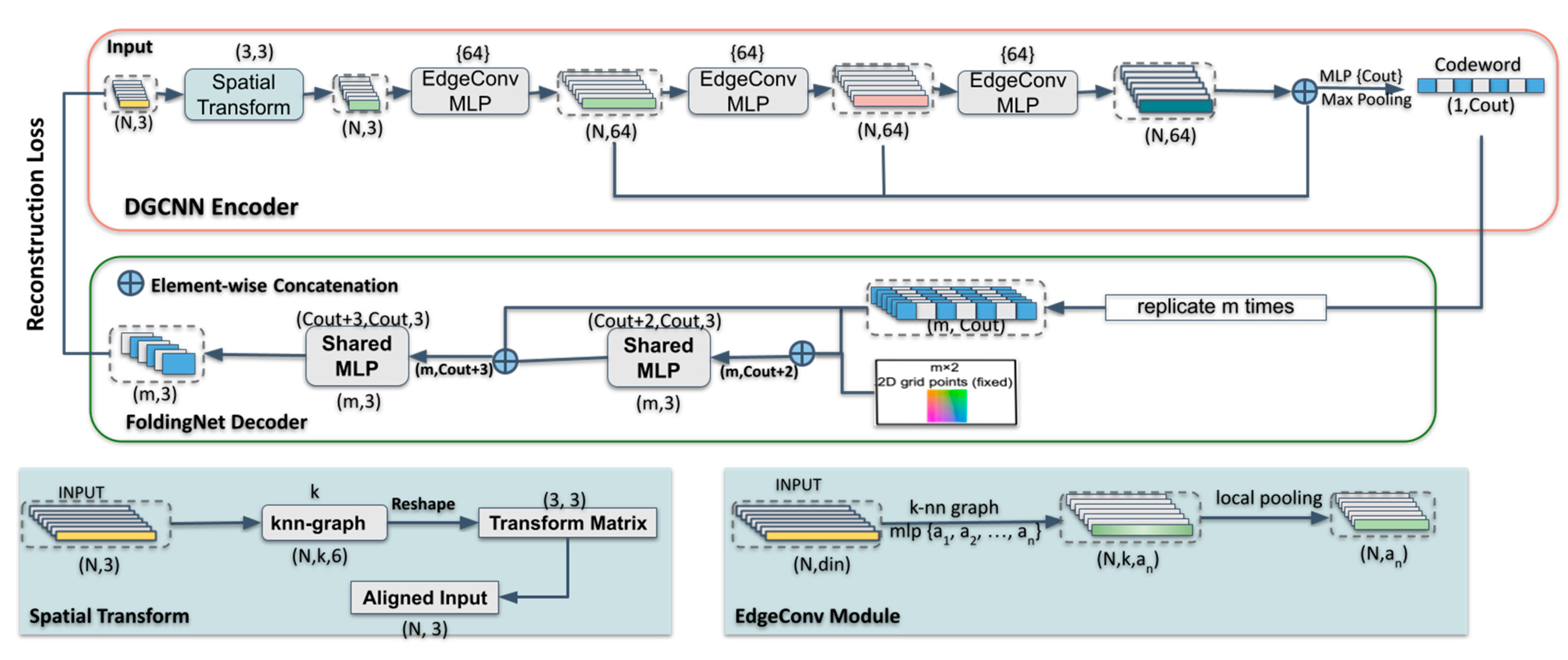
3.1. DGCNN-Based Encoder
3.2. Folding-Based Decoder
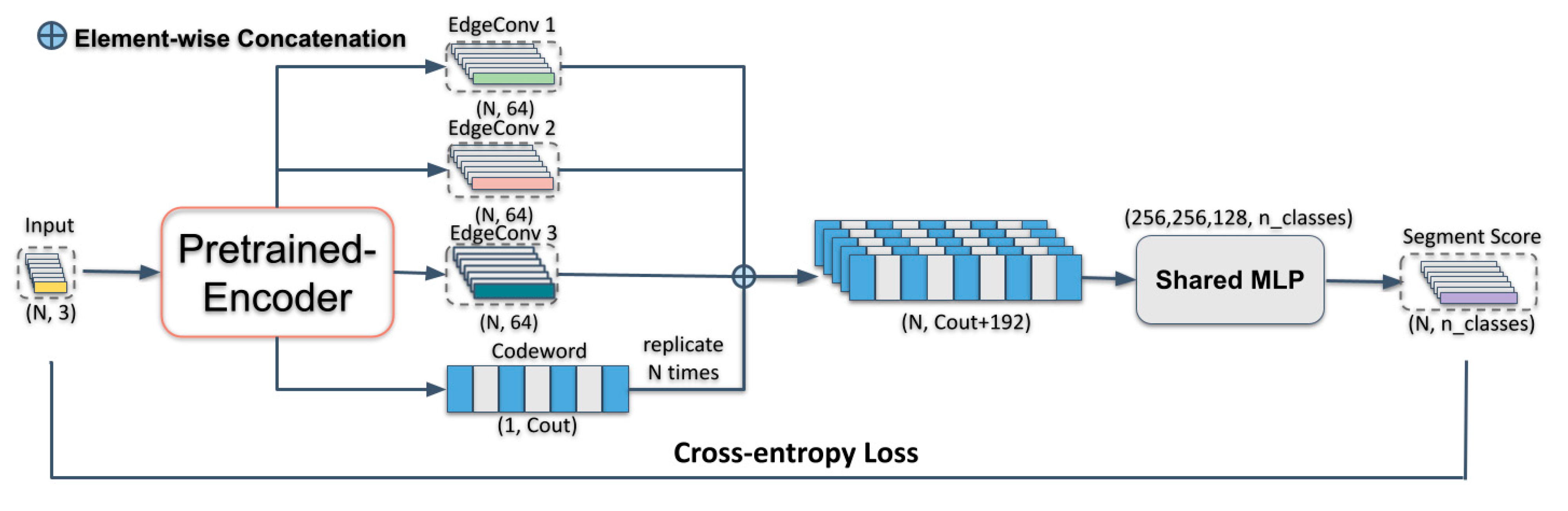
3.3. Semantic Segmentation Network Architecture
3.4. Evaluation Matrix
4. Experiment
4.1. Dataset
4.2. Implementation Details
- Three EdgeConv layers to extract local and global geometric features. The EdgeConv layers take a tensor of shape n × f as input, where f is input features of point cloud, then acquire edge features for each point by applying an MLP with the number of layer neurons defined as . The number of nearest neighbors k is set as 20 at every EdgeConv layer;
- Features generated in three EdgeConv layers are concatenated to aggregate features in different receptive fields; and
- Lastly, the dimension of the MLP layer before the last max pooling layer is set as (512 or 1024) to globally aggregate a 1D global descriptor “codeword” .
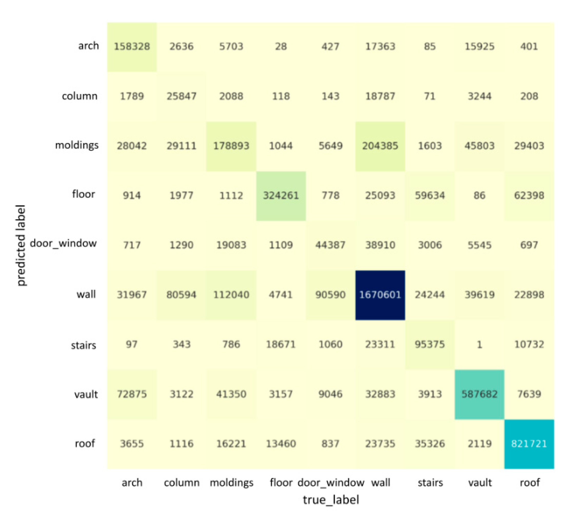
4.3. Results and Analysis
4.4. Ablation Study and Analysis
- The input point size was 2048 in the segmentation training stage; and
- The input point size was 4096 in the segmentation training stage.
- Trained on 2048 points with (x, y, z) coordinates when training the AE and segmentation network;
- Trained on 2048 points with (x, y, z) coordinates when training the AE, and segmentation network training with 4096 points;
- Trained on 4096 points with (x, y, z) coordinates when training the AE, and segmentation network training with 2048 points; and
- Trained on 4096 points with (x, y, z) coordinates when training the AE and segmentation network.
- Comparing rows 1 and 5, rows 2 and 6, rows 3 and 7, and rows 4 and 8, we found that whether 2048 or 4096 points are used as input in the segmentation network with the codeword dimension 512 or 1024, using 2048 points as input in the AE performs much better than if 4096 points are used;
- When analyzing the effect of the input point size in the segmentation network, different results are found: when the dimension of the codeword is 1024, point-cloud size of 2048 in the segmentation network provides better results than 4096; however, when the dimension of the codeword is 512, the segmentation network with a point-cloud size of 4096 outperforms or draws the case of the point cloud with 2048 points; and
- The best overall accuracy (0.773) was achieved when the input point-cloud size was 2048 and 4096 in the AE and segmentation steps, respectively, and was 2.6% better than the second performing network, which had a point-cloud size of 2048 in both steps. However, considering that the training time of the network will be much longer when the input point-cloud size is 4096, in this paper, the experiments were mostly based on input point clouds of size 2048 in both steps.
- The input point feature only contains coordinates ;
- The input point feature contains coordinates and radiometric information ;
- The input point size contains coordinates, radiometric information and geometric information ; and
- The input point size contains coordinates, normalized coordinates’ radiometric information and geometric information , where the normalized coordinate is following the setting in DGCNN_Mod [5].
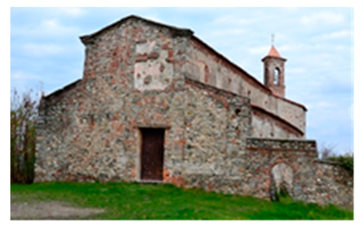
- To add one scene (“4_CA_church”, as shown in Figure 9) as unlabeled training data in the AE training stage;
- To add one scene (“4_CA_church”) as labeled training data in the segmentation network training stage;
- To add one scene (“4_CA_church”) both in the AE and the segmentation network training stage; and
- To decrease the labeled training data size whilst keeping one scene (“7_SMV_chapel_24”) in the segmentation network training stage.
5. Discussion
6. Conclusions
Author Contributions
Funding
Institutional Review Board Statement
Informed Consent Statement
Data Availability Statement
Acknowledgments
Conflicts of Interest
References
- Kutzner, T.; Chaturvedi, K.; Kolbe, T.H. CityGML 3.0: New Functions Open up New Applications. PFG–J. Photogramm. Remote Sens. Geoinf. Sci. 2020, 88, 43–61. [Google Scholar] [CrossRef] [Green Version]
- Löwner, M.-O.; Gröger, G.; Benner, J.; Biljecki, F.; Nagel, C. Proposal for a New LoD and Multi-Representation Concept for CityGML. ISPRS Ann. Photogramm. Remote Sens. Spat. Inf. Sci. 2016, IV-2/W1, 3–12. [Google Scholar] [CrossRef]
- Matrone, F.; Grilli, E.; Martini, M.; Paolanti, M.; Pierdicca, R.; Remondino, F. Comparing Machine and Deep Learning Methods for Large 3D Heritage Semantic Segmentation. ISPRS Int. J. Geo-Inf. 2020, 9, 535. [Google Scholar] [CrossRef]
- Brunetaud, X.; Luca, L.D.; Janvier-Badosa, S.; Beck, K.; Al-Mukhtar, M. Application of Digital Techniques in Monument Preservation. Eur. J. Environ. Civ. Eng. 2012, 16, 543–556. [Google Scholar] [CrossRef]
- Pierdicca, R.; Paolanti, M.; Matrone, F.; Martini, M.; Morbidoni, C.; Malinverni, E.S.; Frontoni, E.; Lingua, A.M. Point Cloud Semantic Segmentation Using a Deep Learning Framework for Cultural Heritage. Remote Sens. 2020, 12, 1005. [Google Scholar] [CrossRef] [Green Version]
- Bosché, F.; Guenet, E. Automating Surface Flatness Control Using Terrestrial Laser Scanning and Building Information Models. Autom. Constr. 2014, 44, 212–226. [Google Scholar] [CrossRef]
- Ham, Y.; Golparvar-Fard, M. Three-Dimensional Thermography-Based Method for Cost-Benefit Analysis of Energy Efficiency Building Envelope Retrofits. J. Comput. Civ. Eng. 2015, 29, B4014009. [Google Scholar] [CrossRef]
- Fazeli, H.; Samadzadegan, F.; Dadrasjavan, F. Evaluating the Potential of RTK-UAV for Automatic Point Cloud Generation in 3D Rapid Mapping. Int. Arch. Photogramm. Remote Sens. Spat. Inf. Sci. 2016, XLI-B6, 221–226. [Google Scholar] [CrossRef] [Green Version]
- Hu, P.; Yang, B.; Dong, Z.; Yuan, P.; Huang, R.; Fan, H.; Sun, X. Towards Reconstructing 3D Buildings from ALS Data Based on Gestalt Laws. Remote Sens. 2018, 10, 1127. [Google Scholar] [CrossRef] [Green Version]
- Czerniawski, T.; Leite, F. Automated Digital Modeling of Existing Buildings: A Review of Visual Object Recognition Methods. Autom. Constr. 2020, 113, 103131. [Google Scholar] [CrossRef]
- Wang, Q.; Kim, M.-K. Applications of 3D Point Cloud Data in the Construction Industry: A Fifteen-Year Review from 2004 to 2018. Adv. Eng. Inform. 2019, 39, 306–319. [Google Scholar] [CrossRef]
- Cao, Y.; Previtali, M.; Scaioni, M. Understanding 3D Point Cloud Deep Neural Networks by Visualization Techniques. Int. Arch. Photogramm. Remote Sens. Spat. Inf. Sci. 2020, XLIII-B2-2020, 651–657. [Google Scholar] [CrossRef]
- Wang, C.; Hou, S.; Wen, C.; Gong, Z.; Li, Q.; Sun, X.; Li, J. Semantic Line Framework-Based Indoor Building Modeling Using Backpacked Laser Scanning Point Cloud. ISPRS J. Photogramm. Remote Sens. 2018, 143, 150–166. [Google Scholar] [CrossRef]
- Kumar, B.; Lohani, B.; Pandey, G. Development of Deep Learning Architecture for Automatic Classification of Outdoor Mobile LiDAR Data. Int. J. Remote Sens. 2019, 40, 3543–3554. [Google Scholar] [CrossRef]
- Huang, J.; Zhang, X.; Xin, Q.; Sun, Y.; Zhang, P. Automatic Building Extraction from High-Resolution Aerial Images and LiDAR Data Using Gated Residual Refinement Network. ISPRS J. Photogramm. Remote Sens. 2019, 151, 91–105. [Google Scholar] [CrossRef]
- Meng, Q.; Wang, W.; Zhou, T.; Shen, J.; Van Gool, L.; Dai, D. Weakly Supervised 3D Object Detection from Lidar Point Cloud. In Proceedings of the European Conference on Computer Vision—ECCV 2020, Glasgow, UK, 23 August 2020; Springer: Glasgow, UK, 2020; Volume 12358, pp. 515–531. [Google Scholar]
- Matrone, F.; Lingua, A.; Pierdicca, R.; Malinverni, E.S.; Paolanti, M.; Grilli, E.; Remondino, F.; Murtiyoso, A.; Landes, T. A Benchmark for Large-Scale Heritage Point Cloud Semantic Segmentation. Int. Arch. Photogramm. Remote Sens. Spat. Inf. Sci. 2020, XLIII-B2-2020, 1419–1426. [Google Scholar] [CrossRef]
- Liu, Y.; Yi, L.; Zhang, S.; Fan, Q.; Funkhouser, T.; Dong, H. P4Contrast: Contrastive Learning with Pairs of Point-Pixel Pairs for RGB-D Scene Understanding. arXiv 2012, arXiv:201213089. [Google Scholar]
- Han, X.; Laga, H.; Bennamoun, M. Image-Based 3D Object Reconstruction: State-of-the-Art and Trends in the Deep Learning Era. IEEE Trans. Pattern Anal. Mach. Intell. 2021, 43, 1578–1604. [Google Scholar] [CrossRef] [Green Version]
- Xie, S.; Gu, J.; Guo, D.; Qi, C.R.; Guibas, L.; Litany, O. PointContrast: Unsupervised Pre-Training for 3D Point Cloud Understanding. In Proceedings of the European Conference on Computer Vision—ECCV 2020, Glasgow, UK, 23 August 2020; Springer: Glasgow, UK, 2020; Volume 12348, pp. 574–591. [Google Scholar]
- Wang, Y.; Sun, Y.; Liu, Z.; Sarma, S.E.; Bronstein, M.M.; Solomon, J.M. Dynamic Graph CNN for Learning on Point Clouds. ACM Trans. Graph. Tog 2019, 38, 1–12. [Google Scholar] [CrossRef] [Green Version]
- Yang, Y.; Feng, C.; Shen, Y.; Tian, D. FoldingNet: Point Cloud Auto-Encoder via Deep Grid Deformation. In Proceedings of the IEEE Conference on Computer Vision and Pattern Recognition, Seattle, WA, USA, 14–19 June 2018; pp. 206–215. [Google Scholar]
- Previtali, M.; Díaz-Vilariño, L.; Scaioni, M. Indoor Building Reconstruction from Occluded Point Clouds Using Graph-Cut and Ray-Tracing. Appl. Sci. 2018, 8, 1529. [Google Scholar] [CrossRef] [Green Version]
- Griffiths, D.; Boehm, J. Improving Public Data for Building Segmentation from Convolutional Neural Networks (CNNs) for Fused Airborne Lidar and Image Data Using Active Contours. ISPRS J. Photogramm. Remote Sens. 2019, 154, 70–83. [Google Scholar] [CrossRef]
- Forlani, G.; Nardinocchi, C.; Scaioni, M.; Zingaretti, P. Complete Classification of Raw LIDAR Data and 3D Reconstruction of Buildings. Pattern Anal. Appl. 2006, 8, 357–374. [Google Scholar] [CrossRef]
- Verma, V.; Kumar, R.; Hsu, S. 3D Building Detection and Modeling from Aerial Lidar Data. In Proceedings of the 2006 IEEE Computer Society Conference on Computer Vision and Pattern Recognition (CVPR’06), New York, NY, USA, 17 June 2006; IEEE: New York, NY, USA, 2006; Volume 2, pp. 2213–2220. [Google Scholar]
- Haala, N.; Brenner, C.; Anders, K.-H. 3D Urban GIS from Laser Altimeter and 2D Map Data. Int. Arch. Photogramm. Remote Sens. 1998, 32, 339–346. [Google Scholar]
- Maas, H.-G.; Vosselman, G. Two Algorithms for Extracting Building Models from Raw Laser Altimetry Data. ISPRS J. Photogramm. Remote Sens. 1999, 54, 153–163. [Google Scholar] [CrossRef]
- Chen, D.; Zhang, L.; Mathiopoulos, P.T.; Huang, X. A Methodology for Automated Segmentation and Reconstruction of Urban 3-D Buildings from ALS Point Clouds. IEEE J. Sel. Top. Appl. Earth Obs. Remote Sens. 2014, 7, 4199–4217. [Google Scholar] [CrossRef]
- Su, H.; Maji, S.; Kalogerakis, E.; Learned-Miller, E. Multi-View Convolutional Neural Networks for 3D Shape Recognition. In Proceedings of the 2015 IEEE/CVF International Conference on Computer Vision (ICCV), Santiago, Chile, 11 December 2015; IEEE: Santiago, Chile, 2015; pp. 945–953. [Google Scholar]
- Ma, C.; Guo, Y.; Yang, J.; An, W. Learning Multi-View Representation With LSTM for 3-D Shape Recognition and Retrieval. IEEE Trans. Multimed. 2019, 21, 1169–1182. [Google Scholar] [CrossRef]
- Yang, Z.; Wang, L. Learning Relationships for Multi-View 3D Object Recognition. In Proceedings of the 2019 IEEE/CVF International Conference on Computer Vision (ICCV), Seoul, Korea, 27 October–2 November 2019; IEEE: Seoul, Korea, 2019; pp. 7505–7514. [Google Scholar]
- Riegler, G.; Osman Ulusoy, A.; Geiger, A. OctNet: Learning Deep 3D Representations at High Resolutions. In Proceedings of the 2017 IEEE/CVF Conference on Computer Vision and Pattern Recognition (CVPR), Honolulu, HI, USA, 21–26 July 2017; IEEE: Honolulu, HI, USA, 2017; pp. 6620–6629. [Google Scholar]
- Wang, P.-S.; Liu, Y.; Guo, Y.-X.; Sun, C.-Y.; Tong, X. O-CNN: Octree-Based Convolutional Neural Networks for 3D Shape Analysis. Acm Trans. Graph. Tog 2017, 36, 1–11. [Google Scholar] [CrossRef]
- Qi, C.R.; Su, H.; Mo, K.; Guibas, L.J. PointNet: Deep Learning on Point Sets for 3D Classification and Segmentation. In Proceedings of the 2017 IEEE/CVF Conference on Computer Vision and Pattern Recognition (CVPR), Honolulu, HI, USA, 21–26 July 2017; IEEE: Honolulu, HI, USA, 2017; pp. 652–660. [Google Scholar]
- Guo, Y.; Wang, H.; Hu, Q.; Liu, H.; Liu, L.; Bennamoun, M. Deep Learning for 3D Point Clouds: A Survey. IEEE Trans. Pattern Anal. Mach. Intell. 2020, 1. [Google Scholar] [CrossRef]
- Zhang, L.; Zhang, L. Deep Learning-Based Classification and Reconstruction of Residential Scenes from Large-Scale Point Clouds. IEEE Trans. Geosci. Remote Sens. 2017, 56, 1887–1897. [Google Scholar] [CrossRef]
- Zhang, L.; Li, Z.; Li, A.; Liu, F. Large-Scale Urban Point Cloud Labeling and Reconstruction. ISPRS J. Photogramm. Remote Sens. 2018, 138, 86–100. [Google Scholar] [CrossRef]
- Hensel, S.; Goebbels, S.; Kada, M. Facade Reconstruction for Textured LoD2 CityGML Models Based on Deep Learning and Mixed Integer Linear Programming. ISPRS Ann. Photogramm. Remote Sens. Spat. Inf. Sci. 2019, IV-2/W5, 37–44. [Google Scholar] [CrossRef] [Green Version]
- Jarząbek-Rychard, M.; Borkowski, A. 3D Building Reconstruction from ALS Data Using Unambiguous Decomposition into Elementary Structures. ISPRS J. Photogramm. Remote Sens. 2016, 118, 1–12. [Google Scholar] [CrossRef]
- Axelsson, M.; Soderman, U.; Berg, A.; Lithen, T. Roof Type Classification Using Deep Convolutional Neural Networks on Low Resolution Photogrammetric Point Clouds From Aerial Imagery. In Proceedings of the 2018 IEEE International Conference on Acoustics, Speech and Signal Processing (ICASSP), Calgary, AB, Canada, 15 April 2018; IEEE: Calgary, AB, Canada, 2018; pp. 1293–1297. [Google Scholar]
- Goodfellow, I.J.; Pouget-Abadie, J.; Mirza, M.; Xu, B.; Warde-Farley, D.; Ozair, S.; Courville, A.; Bengio, Y. Generative Adversarial Networks. In Proceedings of the 27th International Conference on Neural Information Processing Systems (NIPS), Montreal, QC, Canada, 8–13 December 2014; MIT Press: Cambridge, MA, USA, 2014; Volume 2, pp. 2672–2680. [Google Scholar]
- Donahue, J.; Krähenbühl, P.; Darrell, T. Adversarial Feature Learning. arXiv 2016, arXiv:160509782. [Google Scholar]
- Mescheder, L.; Nowozin, S.; Geiger, A. Adversarial Variational Bayes: Unifying Variational Autoencoders and Generative Adversarial Networks. In Proceedings of the 34th International Conference on Machine Learning, Sydney, Australia, 6–11 August 2017; Volume 70, pp. 2391–2400. [Google Scholar]
- Karras, T.; Laine, S.; Aila, T. A Style-Based Generator Architecture for Generative Adversarial Networks. In Proceedings of the 2019 IEEE/CVF Conference on Computer Vision and Pattern Recognition (CVPR), Long Beach, CA, USA, 16–20 June 2019; IEEE Computer Soc.: Long Beach, CA, USA, 2019; pp. 4396–4405. [Google Scholar]
- Hinton, G.E.; Salakhutdinov, R.R. Reducing the Dimensionality of Data with Neural Networks. Science 2006, 313, 504–507. [Google Scholar] [CrossRef] [Green Version]
- Van den Oord, A.; Kalchbrenner, N.; Vinyals, O.; Espeholt, L.; Graves, A.; Kavukcuoglu, K. Conditional Image Generation with PixelCNN Decoders. In Proceedings of the 30th International Conference on Neural Information Processing Systems, Barcelona, Spain, 5–10 December 2016; Curran Associates Inc.: Red Hook, NY, USA, 2016; pp. 4797–4805. [Google Scholar]
- Achlioptas, P.; Diamanti, O.; Mitliagkas, I.; Guibas, L. Learning Representations and Generative Models for 3D Point Clouds. In Proceedings of the 35th International Conference on Machine Learning, Stockholm, Sweden, 10–15 July 2018; PMLR.org: Stockholm, Sweden, 2018; Volume 80, pp. 40–49. [Google Scholar]
- Li, C.-L.; Zaheer, M.; Zhang, Y.; Poczos, B.; Salakhutdinov, R. Point Cloud GAN. arXiv 2018, arXiv:181005795. [Google Scholar]
- Arjovsky, M.; Chintala, S.; Bottou, L. Wasserstein Generative Adversarial Networks. In Proceedings of the 34th International Conference on Machine Learning, Sydney, Australia, 6–11 August 2017; PMLR.org: Sydney, Australia, 2017; Volume 70, pp. 214–223. [Google Scholar]
- Groueix, T.; Fisher, M.; Kim, V.G.; Russell, B.C.; Aubry, M. A Papier-Mâché Approach to Learning 3d Surface Generation. In Proceedings of the 2018 IEEE/CVF Conference on Computer Vision and Pattern Recognition (CVPR), Salt Lake City, UT, USA, 18–23 June 2018; IEEE: Salt Lake City, UT, USA, 2018; pp. 216–224. [Google Scholar]
- Sauder, J.; Sievers, B. Self-Supervised Deep Learning on Point Clouds by Reconstructing Space. In Proceedings of the 2019 Advances in Neural Information Processing Systems (NIPS), Vancouver, BC, Canada, 8–14 December 2019; Curran Associates, Inc.: Vancouver, BC, Canada, 2019; Volume 32, pp. 12962–12972. [Google Scholar]
- Deng, H.; Birdal, T.; Ilic, S. Ppfnet: Global Context Aware Local Features for Robust 3d Point Matching. In Proceedings of the 2018 IEEE/CVF Conference on Computer Vision and Pattern Recognition (CVPR), Salt Lake City, UT, USA, 18–23 June 2018; IEEE: Salt Lake City, UT, USA, 2018; pp. 195–205. [Google Scholar]
- Deng, H.; Birdal, T.; Ilic, S. Ppf-Foldnet: Unsupervised Learning of Rotation Invariant 3d Local Descriptors. In Proceedings of the European Conference on Computer Vision—ECCV 2018, Munich, Germany, 8–14 September 2018; Springer International Publishing AG: Munich, Germany, 2018; Volume 11209, pp. 602–618. [Google Scholar]
- Zhao, Y.; Birdal, T.; Deng, H.; Tombari, F. 3D Point Capsule Networks. In Proceedings of the 2019 IEEE/CVF Conference on Computer Vision and Pattern Recognition (CVPR), Long Beach, CA, USA, 16–20 June 2019; IEEE: Long Beach, CA, USA, 2019; pp. 1009–1018. [Google Scholar]
- Chen, Z.; Yin, K.; Fisher, M.; Chaudhuri, S.; Zhang, H. Bae-Net: Branched Autoencoder for Shape Co-Segmentation. In Proceedings of the 2019 IEEE/CVF International Conference on Computer Vision (ICCV), Seoul, Korea, 27 October–2 November 2019; IEEE: Seoul, Korea, 2019; pp. 8490–8499. [Google Scholar]
- Fan, H.; Su, H.; Guibas, L. A Point Set Generation Network for 3D Object Reconstruction from a Single Image. In Proceedings of the 2017 IEEE Conference on Computer Vision and Pattern Recognition (CVPR), Honolulu, HI, USA, 21–26 July 2017; IEEE: Honolulu, HI, USA, 2017; pp. 2463–2471. [Google Scholar]
- Wu, Z.; Song, S.; Khosla, A.; Yu, F.; Zhang, L.; Tang, X.; Xiao, J. 3d Shapenets: A Deep Representation for Volumetric Shapes. In Proceedings of the 2015 IEEE/CVF Conference on Computer Vision and Pattern Recognition (CVPR), Boston, MA, USA, 7–12 June 2015; IEEE: Boston, MA, USA, 2015; pp. 1912–1920. [Google Scholar]
- Chang, A.X.; Funkhouser, T.; Guibas, L.; Hanrahan, P.; Huang, Q.; Li, Z.; Savarese, S.; Savva, M.; Song, S.; Su, H. ShapeNet: An Information-Rich 3D Model Repository. arXiv 2015, arXiv:151203012. [Google Scholar]
- Munoz, D.; Bagnell, J.A.; Vandapel, N.; Hebert, M. Contextual Classification with Functional Max-Margin Markov Networks. In Proceedings of the 2009 IEEE Conference on Computer Vision and Pattern Recognition (CVPR), Miami Beach, FL, USA, 20–25 June 2009; IEEE: Miami Beach, FL, USA, 2009; pp. 975–982. [Google Scholar]
- Barazzetti, L.; Remondino, F.; Scaioni, M. Combined Use of Photogrammetric and Computer Vision Techniques for Fully Automated and Accurate 3D Modeling of Terrestrial Objects. In Proceedings of the Videometrics, Range Imaging, and Applications X, San Diego, CA, USA, 2 August 2009; Volume 7447. [Google Scholar]
- Fugazza, D.; Scaioni, M.; Corti, M.; D’Agata, C.; Azzoni, R.S.; Cernuschi, M.; Smiraglia, C.; Diolaiuti, G.A. Combination of UAV and Terrestrial Photogrammetry to Assess Rapid Glacier Evolution and Map Glacier Hazards. Nat. Hazards Earth Syst. Sci. 2018, 18, 1055–1071. [Google Scholar] [CrossRef] [Green Version]
- Kingma, D.P.; Ba, J. Adam: A Method for Stochastic Optimization. In Proceedings of the Conference Track Proceedings of 3rd International Conference on Learning Representations, San Diego, CA, USA, 7–9 May 2015; ICLR (Poster) 2015: San Diego, CA, USA, 2015. [Google Scholar]
- Qi, C.R.; Yi, L.; Su, H.; Guibas, L.J. PointNet++: Deep Hierarchical Feature Learning on Point Sets in a Metric Space. In Proceedings of the Advances in Neural Information Processing Systems 30 (NIPS 2017), Long Beach, CA, USA, 4–9 December 2017; Neural Information Processing Systems (NIPS): Long Beach, CA, USA, 2017; Volume 30, pp. 5105–5114. [Google Scholar]
- Atzmon, M.; Maron, H.; Lipman, Y. Point Convolutional Neural Networks by Extension Operators. Acm Trans. Graph. Tog 2018, 37, 71. [Google Scholar] [CrossRef] [Green Version]


| Method | Training Scenes | Test Scene | mIoU | OA |
|---|---|---|---|---|
| PointNet [35] | 10 scenes | Scene_B | 0.114 | 0.35 |
| PointNet++ [64] | 10 scenes | Scene_B | 0.121 | 0.528 |
| PCNN [65] | 10 scenes | Scene_B | 0.26 | 0.629 |
| DGCNN [21] | 10 scenes | Scene B | 0.29 | 0.74 |
| DGCNN [21] | 15 scenes | Scene A | 0.376 | 0.784 |
| DGCNN [21] | 15 scenes | Scene B | 0.353 | 0.752 |
| DGCNN [21] | 3 scenes | Scene A | 0.243 | 0.499 |
| DGCNN [21] | 3 scenes | Scene B | 0.163 | 0.362 |
| Ours | 3 scenes | Scene_A | 0.463 | 0.773 |
| Ours | 3 scenes | Scene_B | 0.408 | 0.666 |
| Method | mIoU | Arch | Column | Molding | Floor | Door–Window | Wall | Stair | Vault | Roof |
|---|---|---|---|---|---|---|---|---|---|---|
| PointNet [35] | 0.114 | 0.000 | 0.000 | 0.001 | 0.294 | 0.000 | 0.411 | 0.000 | 0.337 | 0.094 |
| PointNet++ [64] | 0.121 | 0.000 | 0.000 | 0.002 | 0.009 | 0.000 | 0.514 | 0.000 | 0.074 | 0.608 |
| PCNN [65] | 0.26 | 0.072 | 0.062 | 0.198 | 0.482 | 0.004 | 0.581 | 0.082 | 0.468 | 0.658 |
| DGCNN [21] | 0.29 | 0.060 | 0.064 | 0.142 | 0.470 | 0.006 | 0.603 | 0.290 | 0.520 | 0.845 |
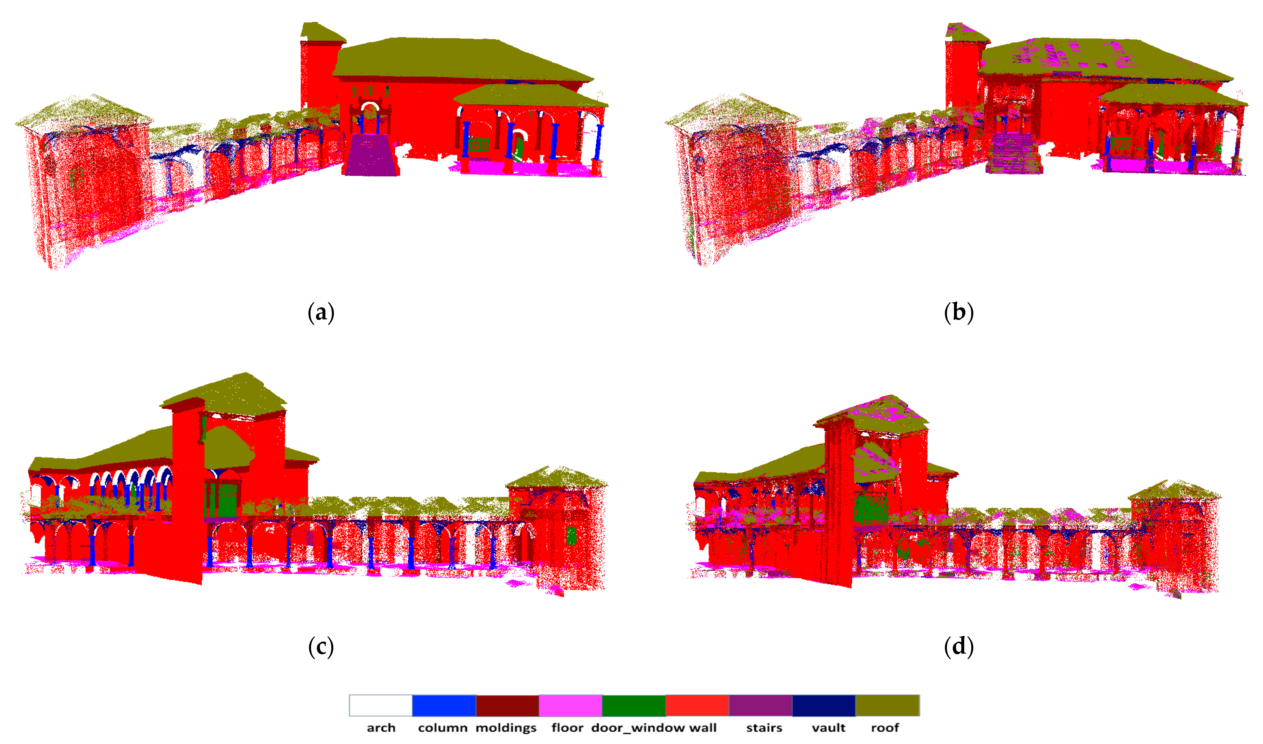
| Ours | 0.408 | 0.880 | 0.243 | 0.117 | 0.471 | 0.005 | 0.676 | 0.035 | 0.577 | 0.659 |
| Encoder | Training Scene | OA 1 |
|---|---|---|
| FoldingNet | 1 scene | 0.425 |
| FoldingNet | 3 scenes | 0.42 |
| DGCNN-based | 1 scene | 0.493 |
| DGCNN-based | 3 scenes | 0.561 |
| Data Augment | OA_Scene_A | OA_Scene_B |
|---|---|---|
| wo_translation | 0.631 | 0.649 |
| w_translation | 0.747 | 0.681 |
| Reconstruction_Loss | Codeword_Dims | AE_n_Points | Seg_n_Points 1 | OA_Scene_A |
|---|---|---|---|---|
| CD | 512 | 2048 | 4096 | 0.773 |
| CD_M | 512 | 2048 | 4096 | 0.71 |
| CD | 1024 | 2048 | 2048 | 0.722 |
| CD_M | 1024 | 2048 | 2048 | 0.71 |
| Codeword_Dims | Seg_n_Points | OA_Scene_A |
|---|---|---|
| 512 | 2048 | 0.747 |
| 1024 | 2048 | 0.722 |
| 512 | 4096 | 0.773 |
| 1024 | 4096 | 0.694 |
| Seg_n_Points | AE_n_Points | Codeword_Dims | OA_Scene_A |
|---|---|---|---|
| 2048 | 2048 | 512 | 0.747 |
| 4096 | 2048 | 512 | 0.773 |
| 2048 | 2048 | 1024 | 0.722 |
| 4096 | 2048 | 1024 | 0.694 |
| 2048 | 4096 | 512 | 0.497 |
| 4096 | 4096 | 512 | 0.494 |
| 2048 | 4096 | 1024 | 0.520 |
| 4096 | 4096 | 1024 | 0.502 |
| Input Feature | OA_Scene_A | mIoU | OA_Scene_B | mIoU |
|---|---|---|---|---|
| DGCNN 1 | 0.784 | 0.376 | 0.752 | 0.353 |
| DGCNN-Mod 2 | 0.896 | 0.535 | 0.837 | 0.470 |
| Ours: | ||||
| 0.747 | 0.459 | 0.681 | 0.383 | |
| 0.700 | 0.433 | 0.693 | 0.384 | |
| 0.815 | 0.513 | 0.764 | 0.464 | |
| 3 | 0.701 | 0.407 | 0.544 | 0.240 |
| AE_Training_Scene | Seg_Training_Scene | OA_Scene_A |
|---|---|---|
| 3_scene | 1_scene | 0.695 |
| 3_scene | 3_scene | 0.747 |
| 3_scene | 4_scene | 0.76 |
| 4_scene | 3_scene | 0.743 |
| 4_scene | 4_scene | 0.772 |
Publisher’s Note: MDPI stays neutral with regard to jurisdictional claims in published maps and institutional affiliations. |
© 2021 by the authors. Licensee MDPI, Basel, Switzerland. This article is an open access article distributed under the terms and conditions of the Creative Commons Attribution (CC BY) license (https://creativecommons.org/licenses/by/4.0/).
Share and Cite
Cao, Y.; Scaioni, M. 3DLEB-Net: Label-Efficient Deep Learning-Based Semantic Segmentation of Building Point Clouds at LoD3 Level. Appl. Sci. 2021, 11, 8996. https://doi.org/10.3390/app11198996
Cao Y, Scaioni M. 3DLEB-Net: Label-Efficient Deep Learning-Based Semantic Segmentation of Building Point Clouds at LoD3 Level. Applied Sciences. 2021; 11(19):8996. https://doi.org/10.3390/app11198996
Chicago/Turabian StyleCao, Yuwei, and Marco Scaioni. 2021. "3DLEB-Net: Label-Efficient Deep Learning-Based Semantic Segmentation of Building Point Clouds at LoD3 Level" Applied Sciences 11, no. 19: 8996. https://doi.org/10.3390/app11198996
APA StyleCao, Y., & Scaioni, M. (2021). 3DLEB-Net: Label-Efficient Deep Learning-Based Semantic Segmentation of Building Point Clouds at LoD3 Level. Applied Sciences, 11(19), 8996. https://doi.org/10.3390/app11198996