A Novel Luminance-Based Algorithm for Classification of Semi-Dark Images

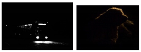
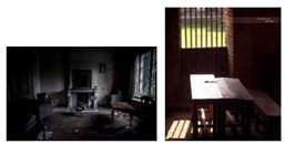
Featured Application

The fundamental research is relevant to several applications involving dynamic conditions in terms of of incoming image’s lightning and overall visibility of content present in it. Some of the applications include surveillance, student authentication in online learning environments, autonomous robotics.

Abstract

Image classification of a visual scene based on visibility is significant due to the rise in readily available automated solutions. Currently, there are only two known spectrums of image visibility i.e., dark, and bright. However, normal environments include semi-dark scenarios. Hence, visual extremes that will lead to the accurate extraction of image features should be duly discarded. Fundamentally speaking there are two broad methods to perform visual scene-based image classification, i.e., machine learning (ML) methods and computer vision methods. In ML, the issues of insufficient data, sophisticated hardware and inadequate image classifier training time remain significant problems to be handled. These techniques fail to classify the visual scene-based images with high accuracy. The other alternative is computer vision (CV) methods, which also have major issues. CV methods do provide some basic procedures which may assist in such classification but, to the best of our knowledge, no CV algorithm exists to perform such classification, i.e., these do not account for semi-dark images in the first place. Moreover, these methods do not provide a well-defined protocol to calculate images’ content visibility and thereby classify images. One of the key algorithms for calculation of images’ content visibility is backed by the HSL (hue, saturation, lightness) color model. The HSL color model allows the visibility calculation of a scene by calculating the lightness/luminance of a single pixel. Recognizing the high potential of the HSL color model, we propose a novel framework relying on the simple approach of the statistical manipulation of an entire image’s pixel intensities, represented by HSL color model. The proposed algorithm, namely, Relative Perceived Luminance Classification (RPLC) uses the HSL (hue, saturation, lightness) color model to correctly identify the luminosity values of the entire image. Our findings prove that the proposed method yields high classification accuracy (over 78%) with a small error rate. We show that the computational complexity of RPLC is much less than that of the state-of-the-art ML algorithms.

1. Introduction

Semi dark imagery is one of the most challenging tasks to be handled by digital image comprehension, as low light covers a huge part of the image data acquisition of an environment. It has relevance to the advanced computer vision applications, such as surveillance, autonomous vehicle [1], farmland classification [2,3], surgical instrument classification [4], medical imaging [5], wildlife tracking [6] and so on. The capability of the human brain for capturing visual information and processing it has evolved to see in the dark, whereas the self-decisive nature of the AI networks is still not equipped to process dark images [7,8]. For the starters of digital image comprehension, the basic task is to classify the incoming image. The classification of images subjected to visibility of the content present is very crucial, as it has the potential to reject the overhead of processing images involving visual extremes. Visual extremes, in the context of content visibility, appear in the forms of bright and dark images, such images reside on the opposite sides of visual spectrums. These images are perceptually difficult to visualize and, hence, automated applications are constrained to process such images. Extracting and eliminating extremely dark and bright images will lead to the preservation of semi-dark images, having visible image features for accurate subsequent processing. Image classification in terms of visual scene visibility is accomplished by two widely used techniques, i.e., machine learning techniques and computer vision (CV) techniques. Both techniques provide limited functionality with perspective of highlighting semi dark images. The ML techniques are limited in their functional discourse due to a number of factors, ranging from data curbing nature, complexity associated with the optimizers, model overfitting issues, model training and testing time, and so on [9,10]. Moreover, the ML methods fail to find relevance among the digital image features, i.e., same image content may appear in all the three conditions (dark, semi-dark and bright). The CV techniques recognizes problem of visibility in terms of the color model being used for image representation [11]. The visibility of an image is directly related to the luminance, which can be identified either by light sensors incorporated in the high definition cameras [7,12,13,14,15] or by manipulating the color model information. The weighted manipulation of an image’s hue, saturation, lightness (HSL) color model leads to the calculation of perceived brightness/luminance of singular pixel of image. The same concept is used for identification of visibility of image. However, there is no well-defined procedure streamlined, so far, for the identification of an entire image’s visibility based on luminance. Moreover, the current image classification models classify images based on luminance into two classes (dark and bright) only [2,16]. This classification fails to highlight the semi-dark scenes, thereby a lot of images incorporating visual extremes become part of subsequent intelligent visual processing. This, eventually, increases processing costs. Unfortunately, semi-dark imagery has not received enough focus of research community as a separate entity in this domain. The image classification based on luminance should highlight semi-dark images besides bright and dark images using HSL color model.

1.1. Gap Analysis & Contribution

The diversity of the visual scene has high impact on the overall performance of categorization of the scene in terms of the visibility of the image [6]. The studies reviewed relating to the automated solutions and visual complexities are limited to controlled visual environments [17] and restricted hardware usage, which means it is difficult to generalize any pattern for the extreme visual interpretative frameworks. Regardless of all the advancements made in the domain of automated image classification, the current knowledgebase in this domain is limited in following aspects:

• Absence of literary and experimental studies relating to the semi-dark visual scenarios.
• Unknown correlating image feature for image classification/categorization of semi-dark images in discourse of ML techniques.
• No well-defined CV classification module for classification of semi-dark images.
• Limited information of luminance based classifying thresholds in CV techniques.

To bridge this gap and classify the huge amount of existing image data representing problem domain data, we present an exclusive study with following aspects:

• Literary analysis of the state-of-the-art image classifiers with respect to luminance and their shortcomings

A critical comparative analysis of existing image classifiers mentioning the problem domain i.e., the illumination of a visual scene. We also discuss the details of these classifiers and their integration with the relevant image feature for image classification. To the best of our knowledge, at the time of writing this manuscript, no study has highlighted this issue and presented such a comparative analysis. This analysis is critical for opening future research directions for better classification of semi-dark images.

2.

Proposal of novel image classification method subjected to correlating image features

An image classification algorithm is presented subjected to the correlating feature, i.e., relative luminance. A luminance-based classification is proposed along with the luminance spectrums backed by manipulation of HSL (hue, saturation, lightness) color model. These spectrums highlight moderate visual scenarios (semi-dark spectrum) for further/subsequent optimal image processing. This helps in elimination of the visual extremes (i.e., dark, and bright) to represent semi-dark images for subsequent processing.

3.

Validation of novel algorithm named Relative Perceived Luminance Classification (RPLC) for image classification based on image luminosity

The proposed luminance-based classification algorithm is extensively validated over variant sized images based on the luminance spectrums. We have also comprehensively presented the design and implementation of novel deterministic protocol based on color model for luminance identification of image to eliminate visual extremes. The presented research formulizes highly tunable algorithm based on simple statistical inference along with the luminosity spectrum values for classification of the images in dark, semi-dark and bright image labels. The benchmarking of the proposed algorithm is performed against CNN and SVM based image classifiers.

4.

Enhancement and labelling of existing datasets using RPLC

For the validation of the proposed algorithm, we extracted images from known datasets of MS COCO [18] and ExDark [19]. After a thorough investigation of visual images, the luminosity values were identified. These findings were further used for annotation of existing visual data. Hence, using the proposed algorithm, we have enhanced and labelled image datasets of MS COCO, Berkeley, and Stanford as dark, semi-dark and bright. We have open sourced the improvised datasets for research community.

To the best of our knowledge, there is not any well-defined method presented so far for the identification/classification of existing images based on the luminance values of the captured visual image. The findings of this work will help in enhanced automation of existing solutions by eliminating the visual extremes before the main working functionality of the intelligent and automated solutions.

1.2. Paper Organization

This paper is organized as follows: Section 2 presents a detailed review of existing literary studies relating to the visual extremes and how the visual data is related to the color model and luminance. This section also mentions all the analytical issues of the existing knowledge along with the gaps in the literature. Section 3 presents detailed research settings of data collection, selection of problem related inference and the framework. Section 4 presents all the extensive experiments for the validation and benchmarking of proposed algorithm. Section 5 mentions the practical implications of the conducted research. Finally, Section 6 conclude the study by putting the identified knowledge in perspective and thereby discussing the future directions.

2. Related Work

For enhancing images to deal with low light scenarios for enhancements of the contrasts various techniques have been used, such as histogram equalization and gamma correction [13]. Some of the advanced techniques include wavelet transform [20] and illumination map estimation [21]. For these techniques to work images are required to have enough information of the scene, i.e., fine grained representation of the content present [13]. Consequently, all the image enhancement techniques fail to deal with the images which incorporate visual extremes (dark, semi-dark, bright) in the scene. This evidence points to the critical need of well-defined illumination-based spectrums to back the working functionality of image processing method for classification of visual scenes.

2.1. Relevance of Color Models to Illumination

Over the years, brightness and luminance have been used interchangeably [11]. The luminance is referred as the falling on the object’s surface. For the existing visual images, luminance of a singular pixel is an achievable concept. The luminance of per pixel can be possibly calculated using information of color model [11]. According to ITU-R BT.601 standard luminosity/luma/luminance can be used as substitution of each other, and its relevant information is identified by weighted manipulation of the RGB channels of the image [22]. Luma is used in known image processing algorithms as backbone for brightness and contrast adjustment. Although the term brightness and luminance are used interchangeably. However, there is huge difference in their mathematical interpretations. For brightness calculation and editing algorithms employ arithmetic mean model, which ends up calculating average of the RGB values. For luminance calculation HSV (hue, saturation, value) or HSB (hue, saturation, brightness) model is used [11]. Another measure of brightness is BCH (brightness, chroma, hue) model [23] which is based on Cohen’s metrics [24] manipulation of the three relevant channel values. The BCH model preserves all the chromatic values of the image for pixel modification for brightness. For brightness and contrast correction a lot of different algorithms such as curves editing, TV based algorithm, lab editing, natural choice have been used, all these algorithms are backed by the color component manipulation by means of exponentials, means, square root and so on [11,25,26]. Another method for calculation of illumination of the visual scene given by ITU-R BT.601 for RGB color space with their relevant weights in overall calculation of luminosity based on RGB pixel values. The influential relevance of color model to the luminance analysis of the scene direct to its usage for classification of visual images.

2.2. Complex Visual Perception Applications

Visual extremes may appear in course of any type of computer aided image comprehension and visual decisive structures. Revolutionized automated systems are now being witnessed in every field from industrial manufacturing of products [27], geosensing of animals [6], astronomy [28], surveillance [29], security [30]. The current research trends are majorly focusing on reducing the effect of factors associated with visual extremes in the automated architectures involved in various application domains. We surveyed literature to analyze the importance of semi-dark imagery in vision-based applications. We used Google Scholar repository to extract articles for the analysis. The survey queries involved keywords, “low light image”, “semi-dark image”, “dark image”, “low luminance image”. The studies chosen were published within the timeframe of 2001 through 2021, uncovering the fact that automation and adversaries have been topic of interest for two decades now. The main reason of this survey is to draw attention to the applications mentioning the effect of luminance in their working discourse. The resulting applications studies present in literature mentioning the constrained automated functionality due to visual extremes are presented in Figure 1.

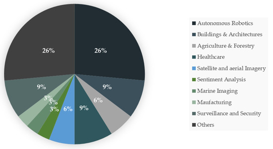
Figure 1. Application Domains involving Visual Extremes.

Figure 1 shows there are over ten different categories of automated applications. Over 26% of the applications focus on the implementation of autonomous robotics and other domains. Whereas 3–9% explicitly focus on healthcare, agriculture, marine imaging, surveillance and so on.

Upon comprehensively analyzing these studies, we found out that despite of all the automated applications striving to provide accurate functionalities, these systems still lack provision of appropriate representations of semi-dark scenarios. These studies have reported the involvement of dynamic luminance conditions as an impeding factor which needs to be addressed. For the correct automated solutions, the incoming visual scene should be duly analyzed for presence of illumination. The classification based on luminance will not only help existing workflows, but it will also help in categorization of existing data. The luminance-based classification identifying the dark, semi-dark and bright refers to the image acquisition environment for all the mentioned applications by representing the scenarios in which image are captured all day long in different lightning conditions. Based on presented analysis and deductions, we hypothesize that up to 50% of these application’s functionality involves low-light imagery which should be properly highlighted to use the counter measures to minimize the associated consequences. This hypothesis is further verified in Section 3.1.

2.3. Related Research Involving Visual Extreme Interpretations

For industrial vision-based applications, a detailed study conducted by Golnabi et al. [27] represents a lot of different applications which includes automated visual inspection, process control (for tracking different documents) in biomedical, pharmaceutical, metal finishing, corrosion detection in pipes, automotive production of assembly lines. Similarly, part identification is another domain for sorting, grading, and identifying different objects in applications. Moreover, some robotic applications are also backed by visual manipulation for smart guidance systems. All these systems are divided into two different categories which are computer vision (CV) based, and machine learning (ML) based approaches.

For visual scene interpretation, CV provides a huge range of methods and algorithms. For such interpretations all the methods at some point must deal with visual extreme where the visual data reaches to extremely low or high light conditions. Lin [31], considered the histogram of visual scenes and identified average difference between the movie frames. The study incorporates the manipulation of spatial coordinates in terms of HSV color model. For automated visual inspection of industrial material, study [32] for component handling image acquisition and enhancement approaches are recommended along with the usage of control systems. This study focuses on circuit board inspection and mentions the possible presence of lightning environments in the workflow. Another study [33], tries to detect dark objects by detecting shadows in digital image. The research mentions the detection of visual extreme, i.e., dark, however, it does not mention the classification of the entire scene. The study just tries to detect apart of shadowy regions using high residual model and reduction of mismatching around boundary region of shadowy parts by using edge matting technique. The study is detailed and revolves around the detection of dark regional parts.

Similarly, a lot of research is conducted over time in the domain of machine learning. In [34], an automated pedestrian detection system is proposed, the proposed setup of the framework uses movement analysis and a support vector machine together to detect the moving pedestrian in semidark environments. The problem with the conducted research is that it is trained and tested in controlled environment of lightning conditions. No mechanism is given for automated identification of image luminance. In [35], a neural network based approach is used for the semantic segmentation of visual scenarios including daytime and night-time scenes. The proposed model adaptation suggests the progressive adaptation of network to be trained on daytime and night-time scenes. The proposed methodology exploits and transfers knowledge from daytime scenes along with large scale annotations. The study mentions the lightning conditions in detail. However, it only covers the external environment under controlled conditions of twilight time and dusk time. There is no proper functionality as some handler in the form of automated solution as part of the model itself. In [36], underwater images are exploited for the semantic segmentation of the marine biological bodies as the underwater images can be dark in nature. The research employs color correction along with the Deeplab V3+ which is deep learning module for segmentation, the research emphasizes on the use of color correction but does not work on the elimination of the luminance extremes such as dark scenes. The referred study only enhances the incoming image using color correction method UCM. In [37], yet another deep learning based framework is used for image dehazing as it mentions some of the information for the exploitation and manipulation of dark color channel prior to the actual functionality of the framework for the semantic segmentation of the images in presence of foggy environment. It mentions the manipulation of dark color channel, however, it does not mention any information relating to the luminance of the scene.

2.4. Constrained Core Functionality Mechanics behind Hi-End Image Classifiers

Computational manipulation of the incoming visual scene for image classification has been topic of research for years now. High end computational machines are expected to classify the image. However, even with high computational costs associated in classification tasks, the end results are below satisfactory. This functionality failure is attributed to the dynamicity (including scene luminance) of the visual environment. Over the years a lot of research has been carried out in the domain of image classification focusing the luminance of the image. Nevertheless, still there is absence of research and methods to computationally classify the image based on luminance of the image. Table 1 presents a critical analysis of conducted research in the domain of image classification, mentioning the issue of luminance and its aftereffects on overall accuracy. The research articles included in the literary analysis are retrieved from Google Scholar. The retrieval queries included “low light image classification”, “semi-dark image classification”, “dark image classification”, and “low luminance image classification”.

Table 1. Critical Analysis of State-of-the-art of Image Classifiers.

Title	Classifier Core	Year	Testing Benchmark	Luminance Mentions	Classification Labels	Observations
Image classification at low light levels [38]	Photon limited image correlation technique. Based on theoretical predictions of the statistics of the correlation signal, Fukunaga–Koontz basis vectors	1986	Artificial character data set	Illumination is calculated by means of photons	Classification characters: A, C, D, E, F, G, H, L, P, R	No relevance to the luminance calculated by HSV color model.
Indoor-outdoor image classification [39]	Classifies image subblocks using histograms in ohta color space. Uses shift invariant DCT. K-nearest neighbor classifier.	1998	Dataset collected and labelled by Kodak	No mentions of illumination of scene	Indoor or Outdoor	Weights are assigned to subblocks based on brightness values. Color and texture classification. Fails to classify images with night time flash photos, hazy white sky.
On image classification: City images vs. landscapes [40]	Low level visual features for classification K-means clustering over histograms of low level features.	1998	VisTex database, Images from Corel stock photo library	Transformation to HSV color space	Categories: forests, mountains, and sunset/sunrise	Considered low level features: color histogram, color coherence vector, DCT coefficient, edge direction histogram, and edge direction coherence vector Higher misclassification rates for dark images.
Application of data mining techniques for medical image classification [41]	Association rule mining. Neural network using back-propagation	2001	Mammographic Image Analysis Society (MIAS) Dataset	No mentions of illumination	Labels: Tumor malignant, benign, Normal	Overcomes the effect of brightness or darkness by using enhancement technique of Histogram equalization.
Image classification: Classifying distributions of visual features [42]	Uses visual features present in the luminance channel. Thresholded Viola–Jones rectangular features (five-dimensional descriptor) Probability distribution for feature-lists	2006	NIST tax forms database	Classifies images based on luminance channels.	Document classification based on the text present in the image	Classifies images without OCR (optical character recognition). No mentions of visual extremes
Improving color constancy using indoor–outdoor image classification [43]	Combination of algorithms (Decision forest) Illuminant estimation algorithms	2008	Funt and Ciurea dataset	Based on illuminant spectral power distribution, sensor spectral sensitivities	Indoor or Outdoor	Controlled environment of conventional sensory camera setup for low, medium and high wavelengths
Intelligent Pedestrian Detection System in Semi-dark Environment [34]	Combines movement analysis and support vector machines. Uses HSV Color Model	2009	Real-time videos were captured.	Uses information of Luminance channel.	pedestrian candidates (human, nonhuman)	Luminance based MSR also largely increase the level noises. Controlled environment in terms of camera and 300 to 500 lux (in luminance)
Affective image classification using features inspired by psychology and art theory [44]	Extract and combine low level features for image emotion classification. Naive bayes classifier	2010	International Affective Picture System (IAPS) Dataset, artistic photographs—art sharing	No mentions of illumination of scene.	Labels: Amusement Anger Awe Contentment Disgust Excitement Fear Sad	Based on features such as color, texture composition and content. Standard deviation is used for calculating contrast of light and dark.
Automatic selection of color constancy algorithms for dark image enhancement by fuzzy rule-based reasoning [45]	Mamdani and Larsen fuzzy inferences for selection of best color constancy algorithm for enhancement of dark images. Enhancement Algorithms: White-Patch (WP), Gray-World (GW), 1st order Gray-Edge (GE1)	2015	SFU Laboratory dataset	Hardware based controlled illuminant	Focuses Image enhancement.	Rules created for twelve image features including seven color and three texture features. Consider only dark images under controlled illuminant
Dirty pixels: Optimizing image classification architectures for raw sensor data [46]	Network on 3 sub-nets: low-level Anscombe network, high-level task-specific network, standard classification network	2017	ImageNet	Hardware based controlled illuminant	Focuses enhancement of low-light images rather than classification.	Controlled environment for image formation model in terms of camera (Nexus 5 rear camera, Nexus 5 rear camera, Google Pixel phone rear camera) used and specific ranges of luminance (2 to 200 lux)
Contrast enhancement of low light image using histogram equalization and illumination adjustment [47]	Histogram equalization, gamma correction to detect low light images.	2018	-	RGB to HSV—Luminance based	Strong low-light image (pixel distribution histogram in range of 0 to 0.5), medium low-light image(pixel histogram distribution in range of 0 to 0.6), shadow effect low-light image(pixel histogram distribution in range of 0.4 to 0.8),	Uses only V(brightness only) channel for further gamma correction and intensity calculation. No mentions of image data used or camera used for image acquisition. Covers low light only without considering dark and bright images (Constrained experiments)
Multispectral RGB–NIR image classification using double channel CNN [48]	Double channel CNN: RGB-CNN and NIR-CNN	2019	RGB-NIR dataset, National Agriculture Imagery Program (NAIP) dataset	Hardware based solution for handling low light imagery conditions.	Categories: country, field, forest, indoor, mountain, old building, street, urban, and water	Controlled environment of modified SLR cameras using visible and NIR filters.
A Smartphone-Based Application Using Machine Learning for Gesture Recognition: Using Feature Extraction and Template Matching via Hu Image Moments to Recognize Gestures [7]	Preprocessing step includes separating object pixels from background, binary conversion, morphological operations, contour retrieval. Template matching for gesture classification.	2019	-	Hardware based luminance calculation	8 hand gestures	Controlled environment backed by smartphone-integrated light sensor to calculate brightness level.
Image classification in the dark using Quanta Image Sensors [49]	Student–teacher learning network for low light image classification solution using Quanta Image Sensors (QIS)	2020	Stanford background, Imagenet	Hardware based illumination calculation based on projected photons	Animal classification in dark images.	CMOS image sensors are used with at least tens of photons per pixel. Controlled sensory environment (iPhone camera).
SAR target classification based on radar image luminance analysis by deep learning [50]	Synthesis aperture radar (SAR) target classification using Deep Learning (Neural Networks)	2020	MSTAR dataset	Hardware based luminance information distribution	SAR target classification	Controlled sensory environment.

The critical literary analysis presented in Table 1 infers that the proper handling of low-level features such as pixel values and color information is probable to enhance the functionality of image classifiers. The automated classifiers struggle to classify image if dark to low lightning condition is involved. Moreover, the state-of-the-art classifying approaches are highly dependent on the type of environment including image acquisition sensor and controlled lightning conditions. Finally, none of the discussed studies solves the classification problem to label image as dark, semi-dark and bright based on the luminance of existing image.

2.5. Analytic Issues in Current Research

The existing research encompassing the visual extremes is found to be limited in the functionality as the conducted research limits the working environments of the subsequent workflow by limiting it to certain camera types used, and certain range of luminance falling range. To the best of our knowledge, there has not been any well-defined approach for the luminance identification of the image after its captured. The issues exist in the literature and appear to be handled by the image processing enhancement techniques by controlling the image acquisition environment which requires human intervention. Additionally, the existing knowledge does not mention definite spectrums for the identification of visual complexities in terms of dark, semi dark and bright images. This results in the glaring unavailability of image datasets which can be referred to deal with such problems. Research for filling these gaps is expected to present simplistic and yet deterministic approach for classification of images based on visual complexities along with the luminance spectrums, which would be a huge contribution for future research.

3. Materials and Methods

3.1. Dataset Formation Protocol

The research on extreme visual scenarios has been slower than most of the other problem areas of machine learning and deep learning. The dataset identification for verification and validation of proposed algorithm is the most crucial part for which two factors have been considered. First, the imagery data encompasses most of the visual extremes as well as moderate scenarios including semi-dark images along with dark and bright scenarios which occur on the opposite sides of visual spectrums. Second, the identified data covers variant sizes of images as the algorithm should have deterministic performance as the incoming data, depending on the image capturing device, is expected to vary.

To successfully conduct the presented research, we have extracted images from two known datasets, i.e., MS COCO and ExDark datasets. ExDark Dataset includes images captured in different lightning conditions ranging from ambient to twilight. The dataset includes exclusively dark and semi dark images, so it does not include bright images. To include images residing over the bright side of light spectrum, images are extracted from MS COCO. The extracted images are then combined and passed to two independent human annotators in the loop to annotate the images based on the visibility of content present in the image in accordance with the relative luminance spectrum. The annotation protocol is set by using the display screen of Dell G7 (model: 7590) laptop with resolution 1920 × 1080 and refresh rate 144 Hz. The screen is kept at 90 degrees with highest brightness of 100% approximating the luminance value up to 300 nits. All the human subjects were seated 450 mm–700 mm apart from the screen with viewing angle of 5°–15°maintaining the perfect ergonomic setup [51]. The annotated images are further matched and only the similar labelled images by all three annotators are included in further experiments to reduce the chances of subjective image annotations. The detailed image dataset development protocol is presented in Figure 2. Finally, for the confirmation of deterministic nature of the algorithms under consideration, two different sets of images with variant number of total images are created.

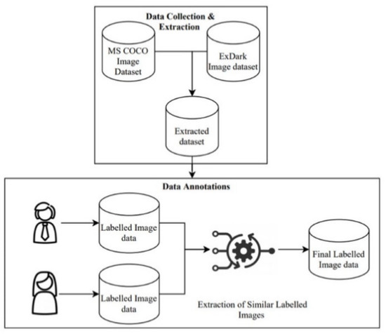
Figure 2. Image Dataset Development Protocol.

This data formation protocol provided basis for the RPLC, after a comprehensive benchmarking analysis we proposed luminance-based classification of existing images explained in Section 3.3 and Algorithm 1. Using the explored facts and figures, we also present enhanced image datasets. The image datasets including MS COCO [18], Berkeley (BSDS-500) [52], Stanford (SBD) [53] are enhanced in terms of dark, semi dark and bright image labels using RPLC. The overall image divisions of these dataset representing the image labels according to RPLC are shown in Figure 3.

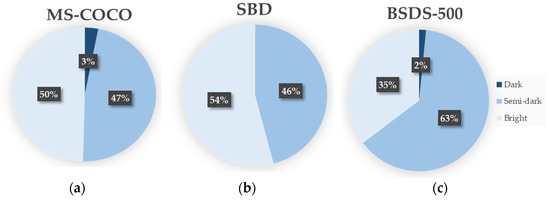
Figure 3. Enhanced Dataset Percentages for Dark, Semi-dark and Bright Images.

The pie charts presented in Figure 3a–c represents the percentages associated to each label and the images present in the respective image data set. The percentages validate the hypothesis that up to half of the imagery data comprises of semi dark scenarios which shall be further processed according to the relevant strategies minimizing the effect of correlating features of semi dark imagery which result in overall degradation of automated solution.

3.2. Problem Centric Rationale Discretion

The classification problem of image identification is based on the visible light spectrum. The visible light spectrum comprises of three different colors, i.e., red, green, blue. For the manipulation of these visual colors, a lot of different color coordinate systems have been used over time depending on the nature of problem to be solved. The problem relating to brightness is closely related to the correct use of these color coordinate systems. The color coordinate system representing the brightness is basically an alternative representation of RGB color model as perceived by the human eye. The color coordinate system used as the core for manipulation of RGB pixel values is hue, saturation, lightness (HSL) [54]. The HSL color model imitates the perceptual color model such as Natural Color System [55]. The color model helps in identification of each pixel of the image. Second challenging factor is to identify the statistical method that retains the consistency of the image lightness and decides the accurate ranges for the classification of Dark, Semi-dark, Bright spectrums based on the perceived lightness of the scene. Initially we attempted to use arithmetic mean of luminosity of pixel values. However, the results of classifications were contradictory to our expectation for the classification. The reason being incorrect inference chosen for the luminosity identification of the image as arithmetic mean neutralizes all the calculated values around the mean value. To assign the image label we then chose inference based on the counters to retain pixel value track of the entire image. Finally, the respective counter having maximum value becomes the image label.

3.3. Inference Core of Luminance-Based Classification

For luminance-based classification as mentioned in section ‘Experimental Setup’, HSL color model is used which allows the lightness calculation of the visual data that is in form of RGB values. For the calculation of perceived lightness of the scene, the values of visible light spectrum falling in electromagnetic spectrum are manipulated and observed for the illumination identification. As the light spectrum comprises of different wavelengths of colors including RGB residing in the visible light spectrum as seen in Figure 2, the same color intensity values of the scene as projected by the camera sensor. These color intensities are converted and calculated for further lightness calculation of the captured scene. The HSL color model identifies pixel luminosity based on Equation (1), we further divide this formula with 255 to keep the luminance value of the pixel in range of 0–1; 0 being the darkest and 1 being the brightest value of the pixel.

$$RL=RL=\frac{0.2125\times R+0.715\times G+0.072\times B}{255}$$

(1)

RL represents the relative luminance of the image pixel being processed. The weights associated to each color channel in Equation (1), are derived from the HSL color model’s details for the calculation of single pixel luminosity. The luminosity calculation is backed by the Photometric/digital ITU BT.709 standardized parameters for conversion of RGB values into respective luminance. The equation refers to luminosity function representing the perceived lightness of the visual scene. The contributors of the lightness have following order green, red and blue, i.e., green component contributes the most whereas blue component contributes the least. Generally, all the associated chromaticity is positive co-efficient which result in RGB to Luminance conversion transformational base. Based on the identified pixel values we performed extensive analysis over the annotated image dataset to finally propose and present the identified spectrums for Dark, Semi-dark and Bright in terms of luminosity of the image.

Figure 4 presents the idea of the electromagnetic spectrum and its part of visible light on top of the visible light spectrum we present novel spectrum identifying the ranges and thereby, these ranges can be used to eliminate visual extremes such as dark and bright.

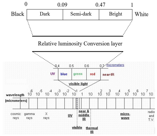
Figure 4. Relative luminance spectrum in visible light.

Based on the identified spectrums we further propose a well defined framework for the classification of existing image data into different categories as suggested by the thresholds. The novel algorithm working at the backend of framework is discussed in Proposed Algorithm 1.

Proposed Algorithm 1: Relative Perceived Luminance Classification

Algorithms 1. Relative Perceived Luminance Classification

Input: An image I of N pixels and spectrum thresholds ${\vartheta }_{DS}$ and ${\vartheta }_{SB}$.

Output: luminance-based label $L$ on image $I$.

1: Pass I with dimensions $H\ast W\ast C$

$C\to Number of color channel$

$C \forall I\to 3$

2: Split $I$ into three multidimensional arrays

$H\ast W\ast R$

$H\ast W\ast G$

$H\ast W\ast B$

Where $H$ represent height, $W$ represent width and $R,G,B$ represent color channel values.

3: Initialize counters $D, SD, B$

4: for each pixel $P$ in $I_{RGB}$

5:     Compute relative luminance $RL$

$RL=\frac{w_{1}R+w_{2}G+w_{3}B}{255}$

$w_1$$, w_2$$, w_3$ are weights associated to $R,G,B$ pixel components of the image.

6:              $\mathbf{if} RL$ $< {\vartheta }_{DS}$

7:                   $D$ + = 1

8:             end if

9:              $\mathbf{if} RL$$< {\vartheta }_{DS}$$\&\& RL$$> {\vartheta }_{SB}$

10:                   $SD$ + = 1

11:             end if

12:              $\mathbf{if} RL$$> {\vartheta }_{SB}$

13:                 $B$ + = 1

14:             end if

15: end for

16: Check counters $D, SD, B$ for maximum value.

17: Label I with L based on maximum value of counter.

The algorithm starts with prior information of existing image and the proposed spectrum details as thresholds ${\vartheta }_{DS}$ and ${\vartheta }_{SB}$, where ${\vartheta }_{DS}$ is threshold between Dark and Semi-dark spectrum and ${\vartheta }_{SB}$ is threshold between Semi-dark and Bright spectrum. For every image pixel having dimensions $H \ast W \ast 3$, 3 being the color channel information every image is iteratively processed for pixel luminosity identification. Here the dimensions of the image explicitly represented by ‘H’ being Height, ‘W’ being Width and ‘3′ represent the associated color channel (RGB) information for further pixel manipulations. For the luminosity calculation, Relative Luminance (RL) calculation formula presented in Equation (1) is employed. According to the identified luminosity of pixel, it is further checked for the criteria of each class (according to the threshold) relevant counters are increased. Finally, the counter with the highest count decides the image label and the resultant is turns out to be the same image with a label, i.e., Dark, Semi-dark, Bright (D, S, B).

The proposed thresholds highlighting the Semi-dark spectrum, besides Dark and Bright, are identified by extensive experiments. The experiments were conducted on different sizes of image datasets to come up with the optimized thresholds for RPLC.

Figure 5 represents accuracies obtained for different tuned thresholds, which led to the identification of final thresholds representing Semi-dark image spectrum.

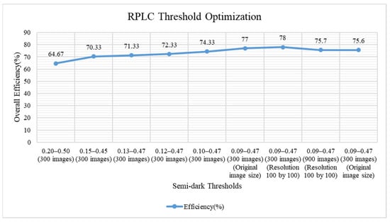
Figure 5. RPLC Threshold rejection & identification.

3.4. Counter Mechanisms for Equalities and Adversaries

The RPLC drives on simplistic approach of the pixel manipulation to reject the visual extremes residing on the either side of the visual spectrum. For the rejection of visual extremes relative luminance of each pixel is computed. The identified thresholds are then compared for each pixel and relevant counters are updated. For the visual scenarios where the counters of two different labels are approximately the same refer to the conditions with equalities. The equalities may appear in image label counters where either the image content is visible, i.e., images close to Bright spectrum or the image content not visible enough, i.e., images close to Dark spectrum. In such scenarios, RPLC picks up image label on random from either of the two labels. This random picking reduces the probability of getting incorrect label by 50%. The relevant proceeding mechanisms shall be than employed to deal with dark, semi-dark or bright images.

Another aspect of implementing RPLC is handlers for adversaries, the simplistic approach is susceptible to the additional noise in the incoming image. The end results can be affected by the addition of simple noise, as the counter mechanism for such conditions RPLC can be accompanied by the image denoising techniques. The image denoising is suggested as the entry stage before the RPLC takes control for the image classification. The incoming images should be filtered before the RPLC iteration. To deal with noises and maintain local image information wide range of denoising techniques are proposed in literature including averaging, median and adaptive filtering techniques. The filtering and denoising technique shall be identified by the nature of the application and its associated noisy images. The critical applications should first remove instances of noise and then pass the filtered images for classification of images based on their luminance and visibility of content.

4. Comparative Analysis of RPLC with CNN through Experimental Validation

4.1. Comparative Pipelines for Image Classification

The experimental validation and benchmarking of the proposed algorithm is achieved by comparing it with the state-of-the-art image classification approaches of convolution neural network (CNN) and support vector machine (SVM). The validation is based on the extensive study of comparison of our proposed algorithm. The experimental study included huge number of iterations for identifying the thresholds as represented by Figure 3. After threshold identification for validation, we kept in mind criteria such as size of dataset, image size (in terms of image resolution). The pipeline for image classification used by CNN, SVM, and luminance based algorithm is shown in Figure 4, Figure 5 and Figure 6 respectively.

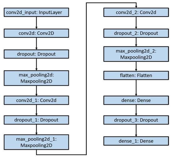
Figure 6. Basic CNN Model Structure for Image Classification.

Figure 6 represents the graphical visualization of the CNN model that has been used for the classification of image in Dark, Semi-dark and Bright categories. The convolutional layer and maxpooling layers used in the pipeline serves the purpose of reducing the spatial size of the incoming image and captures the small details of the scene and tries to decrease the computational power required to process data. The layers used in the CNN helps in extraction of dominant features. Another group of these layers including convolutional, dropout and maxpooling with stride 2 × 2 stride is used to capture low level details even further and finally Dense layer is used to make final prediction about the incoming image in the form of three classes, i.e., Dark, Semi-dark, and Bright.

Figure 7 represents the graphical visualization of SVM pipeline. The incoming image having the label, i.e., Dark, Semi-dark, Bright, is converted into arrays and preprocessed to retain a uniform image size to avoid mismatched image size classification problems. The image dataset is divided into training and testing sets, the SVM classifier is trained and subsequently used for the prediction of image labels.

Figure 7. Support Vector Machine (SVM) Classification Pipeline.

Figure 8 represents the graphical visualization of the RPLC algorithm. The image is manipulated based on the pixel intensities counter are set and updated according to the presence of pixel intensities in terms of Dark, Semi-dark, and Bright. The counter having the highest value is finally taken as the image label.

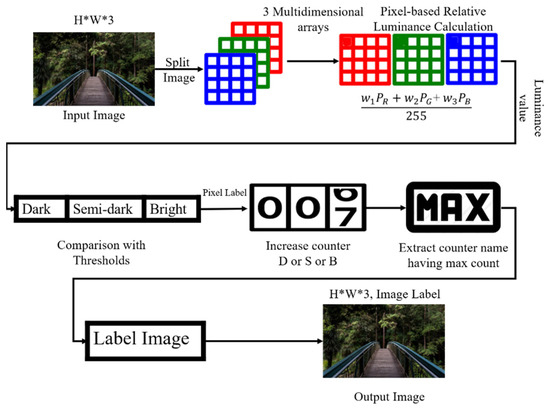
Figure 8. RPLC Pipeline for Image Classification.

4.2. Preparation and Experimental Setup

For experimental setup, the image data is prepared in two different set of images along with the annotations representing Dark, Semi-dark and Bright images. The two sets comprise of a total of 300 and 900 images, vice versa. These set of images, as mentioned earlier, are extracted from ExDark dataset and MSCOCO dataset, both these datasets comprise of variant sized images. To handle the variability of image sizes we considered two different scenarios representing the size of images. The scenarios under consideration are rescaled versions of the images. The first scenario with resolution of 100 by 100 size, and for the second scenario scaled version of 640 by 640 is considered with the zero padding. The addition of zero padding is employed, so that the stat of the art approaches used for validation, i.e., basic CNN and SVM obtains the same size of images of training, testing and validation. However, our proposed algorithm, implying minimum conditions for classification, can classify the images as they appear with whatever the resolution of image is given as input. In addition to that, the proposed algorithm is robust and simplistic enough to work with small amount of image data and large amounts as well. Whereas, for basic CNN to work, we divided the images set in further subsets for training, testing and validation sets. The subsets for image set having a total of 300 is divided into 225 images for training, 45 images for testing, and 25 images for validation set each. The subsets for image set having a total of 900 is divided into 675 images for training, 135 images for testing, and 90 images for validation set each. To increase the dataset size for CNN training to infuse versatility and better training, python library Keras has been used. The ImageDataGenerator method provide by Keras applies data augmentation steps to increase the dataset size and thereby integrates versatility in the network. The data augmentation strategies are applied on all the phases training, testing and validation such that the augmented training images do not vary with a huge margin as compared to the testing and validation images. The augmentation applied on all—training, testing, and validation—maintains the uniformity throughout the experiment. For the augmentation, image pixel normalization is employed to standardize pixel values for fitting and evaluating the CNN. Augmentation methods such as vertical shift, horizontal shift, shear, zoom, and horizontal flips are used. The resultant augmented dataset size is ≈21,600 images, based on the actual number of samples divided by the batch size for the network, i.e., 900/15 equals 60 images per epoch and the total epochs are 60. Moreover, we have six different augmentation operations, the final number of images becomes approximately equals 60 × 60 × 6 images. Finally, for SVM the dataset is divided by ratio of 60:40 implying 60% images for training and 40% images for testing for both dataset sizes. For experiments, google collab has been used with the device type ‘CPU’ and memory limit of 268,435,456 to process the images.

4.3. Benchmarking Analysis

Following the discussed experimental setup, for the validation of RPLC we tested the classification accuracy against basic CNN, support vector machines (SVM). The proposed classification is backed by extensive experimentation for identification of luminosity thresholds based on the annotated dataset images in terms of Dark, Semi-dark and Bright images. After a lot of considerate and meticulously organized experimentation, we introduced the thresholds in form of luminosity spectrums for Dark, Semi-dark and Bright spectrums. The presented spectrums are 0–0.09 for Dark, 0.09–0.47 for Semi-dark, and 0.47–1 for Bright, as shown in Figure 4. For the basic CNN and SVM classification, the requirement is annotated data for classification startup. Whereas, for RPLC the only requirement is prior knowledge of predefined thresholds of each spectrum.

The experiments for validation and benchmarking included two scenarios of different image dataset sizes. For the first scenario, where the dataset size under consideration was 300, Table 1 shows the comprehended accuracies and related logistics.

Table 2 presents the accuracies obtained by basic CNN, SVM and luminosity based classification. For Basic CNN, the epochs used are 60, optimizer used is ‘adagrad’ and batch size is 15, whereas images sizes are kept 100 by 100 and 640 by 640. For SVM the optimizer used is ‘Linear’ along with the images of sizes 100 by 100 and 640 by 640. For luminosity-based classification there are minimal requirements are imposed and image sizes considered for experiments are 100 by 100 and the actual image size. The accuracy obtained by the CNN is 73.3% for training and the validation accuracy is 64.4% for image sizes of 100 by 100 whereas it is clearly seen that training loss is 56% and validation loss of the network is 100%. Similarly, CNN performance for image sizes of 640 by 640 is not any better. The accuracy is 53% and validation accuracy is 71.1% along with the training loss of 83% and validation loss of 100%. The acquired accuracy cannot be trusted for the classification as the losses associated are high which means there is high probability of getting incorrect results. As these classifications can be part of sophisticated and crucial image based applications, we cannot allow this much high error rate to propagate further. The Classification accuracy attained by SVM is 72.5% for image sizes 100 by 100 and 73.3% for image sizes 640 by 640. The accuracy is better than CNN. However, annotations and a high training cost are involved with the usage of SVM. The accuracy obtained by RPLC is 78% for image size of 100 by 100 and the accuracy obtained for actual image size is 77%. The obtained accuracy deduces the algorithm is highly predictable and consistent in nature even for various image sizes.

Table 2. Performance Comparison of RPLC.

Scenario ID	Classifier	Epochs	Batch Size	Image Size	Dataset Size	Optimizer/Kernel	Accuracy		Loss
1	Basic-CNN	60	15	100 × 100	300	adagrad	Acc	Val_Acc	Loss	Val_Loss
							73.3%	64.4%	56%	100%
2	Basic-CNN	60	15	640 × 640	300	adagrad	Acc	Val_Acc	Loss	Val_Loss
							53%	71.1	83%	100%
3	SVM			100 × 100	300	Linear	72.5%		-
4	SVM			640 × 640	300	Linear	73.3%		-
5	RPLC	-	-	100 × 100	300	-	78%		-
6	RPLC	-	-	Actual image size	300	-	77%		-

Table 3 presents the accuracies obtained for image dataset of size 900 images. With the similar CNN architecture and hyperparameters as used earlier, the accuracy turn out to be 40% training accuracy and validation accuracy of 70% of image size of 100 by 100. Classification accuracy for image size 640 by 640 is found to be 66.7% whereas validation accuracy turns out to be 75.5%. While the losses associated are again witnessed to have higher in numbers as compared to the accuracies obtained. Similar CNN architecture with added data augmentation features to increase the dataset size is trained to check the resultant accuracy and associated losses. The data augmentation involved rescaling, width shifting, height shifting, shear, zoom and horizontal flipping. The rescaling range is set to 1/255, width and height shifting are made up to 10% by setting the argument value to 0.1. Similarly, zooming and shearing of 10% is employed. Finally, horizontal flip is also employed in the augmentation process. This makes up to six different augmentation processes. Using this data augmentation scheme. The CNN was trained for two different image sizes, i.e., 100 by 100, and 640 by 640, the resulting accuracies turned out to be 60% accuracy and 73% validation accuracy for image size 100 by 100. Whereas, for image sizes 640 by 640 the obtained accuracy is up to 66% and validation accuracy is 68.8%. The associated losses in both the scenarios are still very high. The accuracy plots are further discussed for detailed analysis in Figure 7. The resultant accuracies of SVM are higher this time, it retains accuracy up to 85% for both the scenarios involving different image sizes. The ML classifiers (CNN and SVM) used for the experimentations are highly dependent on the annotated data and training phase is slow [39]. For the addition of even a single class in these models entire retraining is required [42]. However, for RPLC does not impose prior restrictions for classification. The proposed algorithm RPLC keeps its accuracy intact and drops by a smaller margin and still retains accuracy up to 75.7%. The performance accuracy stats presented in Table 1 and Table 2 infer that the proposed algorithm is deterministic in nature for classification of images and is highly predictable having well-defined and simple protocol to follow for classification of dynamic images. The dynamicity ranges for variant image sizes and number of images to be classified.

Table 3. Performance Comparison of RPLC.

Scenario ID	Classifier	Epochs	Batch Size	Image Size	Dataset Size	Optimizer	Accuracy		Loss
7	Basic-CNN	60	15	100 × 100	900	adagrad	Acc	Val_Acc	Loss	Val_Loss
							40%	70%	100%	100%
8	Basic-CNN	60	15	640 × 640	900	adagrad	Acc	Val_Acc	Loss	Val_Loss
							66.7%	75.5%	76.06%	97.7%
9	Basic-CNN	60	15	100 × 100	≈21,600 with augmentation	adagrad	Acc	Val_Acc	Loss	Val_Loss
							60%	73%	81%	100%
10	Basic-CNN	60	15	640 × 640	≈21,600 with augmentation	adagrad	Acc	Val_Acc	Loss	Val_Loss
							66.7%	68.8%	85.2%	100%
11	SVM			100 × 100	900	Linear	85%
12	SVM			640 × 640	900	Linear	85%
13	RPLC	-	-	100 × 100	900	-	75.7%		-
14	RPLC	-	-	Actual image size	900	-	75.6%		-

We further discuss in detail the possibilities and consequences of CNN being chosen as the backbone for the classification of visual data including visually extreme environments.

Figure 9a–f presents the accuracy plots for training and validation of the CNN for different scenarios.

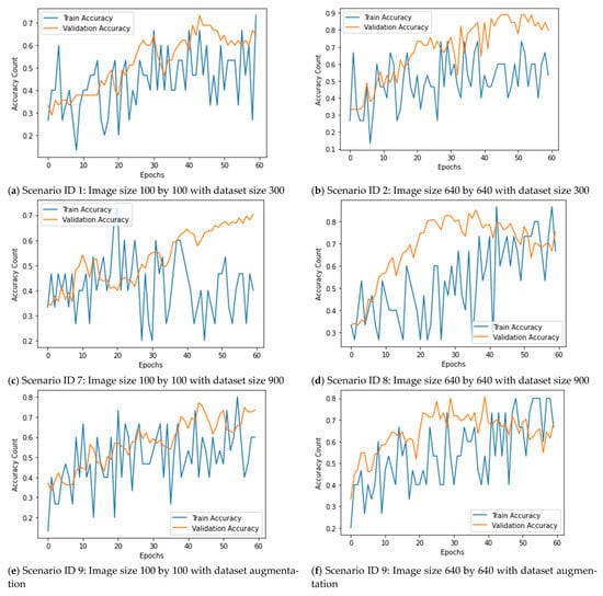
Figure 9. Accuracy plots of basic CNN.

For the experimental setup and CNN architecture construction the python library that has been used is Keras and Tensorflow. Generally, for assessing the network performance the criteria are with increasing epochs the accuracy should be increasing whereas the loss is expected to decrease to ensure that network is working optimally. All the accuracy plots presented in Figure 7 shows differing facts about the network performance. The network performance is fluctuating with the increasing epochs and the losses reach to 100%, as mentioned in Table 2 and Table 3. This means the network is not performing as desired and for such situations the network is usually overfitted, and it is highly likely that such networks result in misclassified results when any new data is classified.

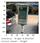
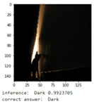
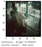
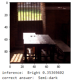
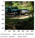
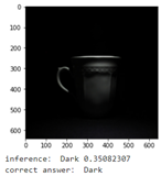
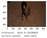
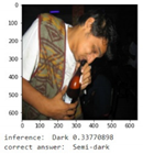
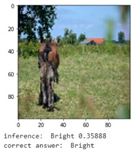
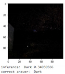
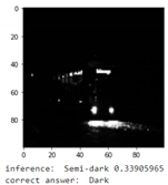
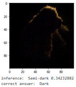
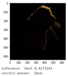
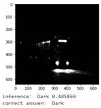
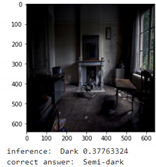
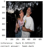
Table 4 shows some of the detailed results of images along with the inferences as acquired by the network and their actual or correct label as annotated by the human annotator.

Table 4. Classification results of Basic CNN under Different Scenarios.

Scenario ID	Correctly Classified		Incorrectly Classified
1 (Basic CNN—Image size 100 by 100, Dataset size 300)
2 (Basic CNN—Image size 640 by 640, Dataset size 300)
7 (Basic CNN—Image size 100 by 100, Dataset size 900)
8 (Basic CNN—Image size 640 by 640, Dataset size 900)

Table 4 shows the experimental results of CNN and with increasing resolution similar images are witnessed to get correct classification results by the CNN. The reason of such altering results is absence of coherence between the input features. CNN seems unable to decide the correct class labels for low resolution images (refer 3rd and 4th row in Table 4). For scenario Id 7, the Dark images, as annotated by an expert, are misclassified to be Semi-dark images, whereas the same images are classified correctly if the network is trained over high resolution images with the same image labels. This uncovers the fact that with increased resolution of images along with higher training times, CNN performs differently as opposed to the network trained on the low resolution images.

Table 5 shows the classification results of RPLC for the similar images as reported by CNN.

Table 5. Classification results of RPLC.

Specification of Luminance-Based Algorithm	Row ID	Correctly Classified	Incorrectly Classified
Luminance spectrum values Dark 0–0.09 Semi-dark 0.10–0.47 Bright 0.48–1, Actual Image Size	1	Bright
			RPLC Label: Bright Correct Answer: Semidark
	2	Semi-dark
			RPLC Label: Semidark Correct Answer: Bright	RPLC Label: Dark Correct Answer: Semidark
	3	Dark
			RPLC Label: Dark Correct Answer: Semidark

The tests are performed over the actual image sizes provided in image dataset without any preprocessing. Row 1, 2, 3 shows the classification results of bright images along with the misclassified results for Dark, Semi-dark, and Bright images, as interpreted by a human annotator.

To further validate the results, we take the confusion matrices of the classification generated by CNN and luminance based algorithm for the test case focusing 300 image datasets for the analysis of percentages for correct and incorrect classification rate. The respective confusion matrices in percentage form for total count of images in each case are shown in Figure 10.

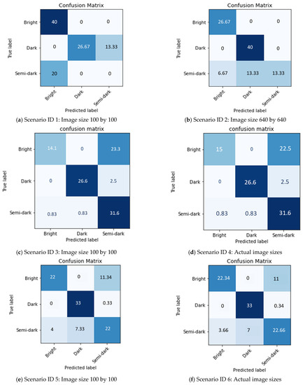
Figure 10. Percentage form confusion matrix of basic CNN (a,b), SVM (c,d), and RPLC (e,f).

The numeric forms of the confusion matrices obtained from the experimental validation were converted in percentage forms for the sake of uniformity in argument. In Figure 10a the percentage of correctly classified images is about 66.76%, whereas incorrectly classified images are up to 33.33%. For Figure 10b the percentage of correctly classified images is 80% and incorrectly classified images hold 20%. In Figure 10c the percentage of correctly classified images is up to 72% whereas incorrectly classified images are approximately around 27.5%. For Figure 10d the percentages for correct and incorrect classification are 73% and 26.6%, respectively. For Figure 10e,f the correctly classified percentage count is up to 77% and 78% and the percentage count for incorrectly classified images is 23% and 22%. Here again RPLC algorithm retains its consistency for the image classification. One of the aspects of presented analysis worth mentioning is that the confusion matrices differ in number of total number of samples used. As the requirements imposed by the CNN includes the division of dataset into small subsets of training, testing and validation the correct and incorrect accuracies as mentioned in Figure 10a,b represents only the validation set whose sizes is 25 images only. Similarly, the confusion matrices for SVM presented in Figure 10c,d represents only the stats for testing set which is 40% of the total image dataset size. This implies there are higher possibilities of obtaining incorrect results for larger datasets whereas the confusion matrix shown for luminance-based algorithm has a total of 300 images which is the total amount of images used for that scenario.

For the discourse of gains achieved relating to the luminance-based algorithm over the CNN based approach for the classification of images, further discussion on the numeric analysis is presented in Table 2 and Table 3.

For the gain calculation presented in Table 6, difference of accuracies among luminance-based and CNN based classification is calculated, after which the difference is divided by the accuracy of CNN based classification accuracy to generate gain of RPLC algorithm over the CNN based classification. For the comparison of Scenario Id 5 v/s 7, the accuracy gains are observed to reach approximately 89.25% for the training set and 8.14% for the testing set. Whereas, even for worst case RPLC algorithm still achieves 0.13% better performance for the validation set as compared to CNN based algorithm.

Table 6. Gain analysis of RPLC algorithm over CNN based classification.

Comparisons of Scenarios (S_ID)	Image Size	Dataset Size	Luminance-Based Classification (RPLC)	CNN-Based Classification		Gain in % Age of Luminance-Based v/s CNN-Based Classification
S_ID 1 v/s S_ID 5	100 × 100	300	78%	Acc	Val_Acc	Acc	Val_Acc
				73.3%	64.4%	6.41%	21.11%
S_ID 2 v/s S_ID 6	640 × 640 v/s Actual Image Size	300	77%	Acc	Val_Acc	Acc	Val_Acc
				53%	71.1	45.2%	8.2%
S_ID 7 v/s S_ID 11	100 × 100	900	75.7%	Acc	Val_Acc	Acc	Val_Acc
				40%	70%	89.25%	8.14%
S_ID 8 v/s S_ID 12	640 × 640 v/s Actual Image Size	900	75.6%	Acc	Val_Acc	Acc	Val_Acc
				66.7%	75.5%	13.34%	0.13%

Following the same calculation pattern for gain identification. Table 7 represents the stats of accuracy gains of RPLC over SVM. For S_ID 3 v/s S_ID 5 and S_ID 4 v/s S_ID 6, RPLC retains positive gain margins whereas for the latter one gains hits negative numbers. However, RPLC’s simplicity, extensibility, speed and consistent performance with minimum prior knowledge for deployment remains a plus point.

Table 7. Gain Analysis of RPLC Algorithm over SVM Classification.

Comparisons of Scenarios (S_ID)	Image Size	Dataset Size	Luminance-Based Classification	SVM-Based Classification	Gain in % Age of Luminance-Based v/s SVM-Based Classification
S_ID 3 v/s S_ID 5	100 × 100	300	78%	72.5%	7.5%
S_ID 4 v/s S_ID 6	640 × 640 v/s Actual Image Size	300	77%	73.3%	5.04%
S_ID 9 v/s S_ID 11	100 × 100	900	75.7%	85%	−10.09%
S_ID 10 v/s S_ID 12	640 × 640 v/s Actual Image Size	900	75.6%	85%	−11%

The extensive experimentation along with the gain analysis of RPLC over the state-of-the-art ML approaches shows that for accurate functionality of these methods massive amount of annotated data covering the problem domain is required. Since synthetic augmentation of the labelled images fails to add to the performance accuracy and has its own drawbacks, such as overfitting (for detailed read over of the associated risks of augmentation refer to studies [56,57]), therefore, as a mitigation strategy to deal with annotation problem of the images RPLC can be used to annotate the data using the proposed thresholds. For extended research, a novel CNN network can also be created, incorporating the information of RPLC and its thresholds in the network parameters to create hybrid approach. Finally, the overall change in performance for classification of images can be examined.

5. Discussion

5.1. Comparative Analysis on Computational Complexity

For the complexity analysis, neural networks consume a lot of computational power depending on the depth of the network. The proposed RPLC algorithm is based on just the matrix multiplication of image with HSL color conversion formula. Putting all that information in simpler words, if image ‘$I$’ comprises of three color channels for the elementary operation of matrix multiplication provided the matrices are square matrices, the time complexity is almost $O\left(n\ast 3\right)$ where n is size of image (digits present in the matrix). Whereas, for the CNN (feed forward in nature), assuming all the different layers of convolution, pooling, dropout along with the added complexity of activation function in each layer; the computational complexity is proportional to $O\left(n^{No. of layers}\right)$. The implementation of CNN used for the experiments include up to 9 layers so we can expect O(n⁹). Finally, the computational complexity associated with the Support Vector Machines for image classification it is approximated to $O\left(2\left(k+1\right)n\right)$, where ‘$k$’ represents piecewise linear approximations of degree 1 and ‘$n$’ represents number of input dimensions [58].

5.2. Practical Implications

The practical implication of the research encompasses a wide range of applications, ranging from autonomous vehicles, healthcare, agriculture, security, and surveillance [59]. All these applications usually include visual extremes, the proposed luminance-based algorithm is probable to add in digitization and automation of these applications. The revolutionization may arise with digitized healthcare, SMART manufacturing and agriculture, architectural sustainability, and so on. All these automated applications can incorporate this algorithm as a mini framework for the elimination of visual extremes.

In addition to that, the novel luminance-based algorithm can aid to classification of existing images in dark, semi-dark and bright images, thereby reducing the costs of creating sheer number of annotations. Using the proposed algorithm, we also introduced well-known datasets, i.e., MSCOCO [18], Berkeley [52] and Stanford background [53] dataset, with enhanced features by including the classification labels for Dark, Semi-dark and Bright images.

6. Conclusions and Future Works

6.1. Conclusions

In this paper, we propose a novel framework based on luminance spectrums for the identification of the visual images based on the presence of brightness/luminance for classification of images as dark, semi-dark, and bright. Later, we propose a well-defined and consistent protocol to classify the visual data based on the luminance presence. The luminance is computed using the known HSL color model recommended by ITU-BT.709 primaries. On top of the individual manipulation of RGB color space, we introduce an off-the-shelf method for identification and calculation of luminance for entire visual image rather than just a singular pixel. The proposed Relative Perceived Luminance Classification (RPLC) algorithm along with the luminance spectrums are extensively tested against the state-of-the-art approaches of convolutional neural network and support vector machine. The benchmarking results verified that the performance of proposed algorithm RPLC is better than CNN. Additionally, it has higher reliability and consistency in rates of accuracy for the classification of images in terms of Dark, Semi-dark and Bright images. The proposed algorithm RPLC achieved accuracy up to 78% and it can be further tuned to get better classification accuracy. The results show that RPLC outperforms CNN based and SVM-based Classification. The gain margin of RPLC over CNN is 89.25% for the training set and 8.14% for the validation set. Whereas, for SVM it is up to 7.5% with bare minimum prior requirements of implementation. Finally, the computational complexity of RPLC is substantially less than the CNN-based and SVM classification algorithm.

6.2. Future Work

The experimental research demonstrates the approach based on the luminance identification of the image against the state-of-the-art approach of CNN fails to perform up to the mark and results in higher error rates. The reasons for the CNN working functionality failure can be attributed to the irrelevance and absence of the coherence of the visual scene. This limits the functionality of CNN for finding the relevance among the visual scenes. Whereas, for the proposed luminance-based algorithm, it impeccably processes images and generates consistently correct labels for the images in dynamic scenarios. For the extension of conducted research, the luminance spectrums can be further tuned to achieve even better classification accuracy. Moreover, image datasets of versatile nature, such as marine datasets or industrial datasets, can be further experimented for the validation and relevance of the proposed luminance spectrums.

References

- McAllister, R.; Gal, Y.; Kendall, A.; Van Der Wilk, M.; Shah, A.; Cipolla, R.; Weller, A. Concrete Problems for Autonomous Vehicle Safety: Advantages of Bayesian Deep Learning. In Proceedings of the International Joint Conference on Artificial Intelligence, Melbourne, Australia, 19–25 August 2017; Available online: https://www.ijcai.org/proceedings/2017/0661.pdf (accessed on 17 August 2021).
- Zhang, F.; Hu, Z.; Fu, Y.; Yang, K.; Wu, Q.; Feng, Z. A New Identification Method for Surface Cracks from UAV Images Based on Machine Learning in Coal Mining Areas. Remote Sens. 2020, 12, 1571. [Google Scholar] [CrossRef]
- Milioto, A.; Lottes, P.; Stachniss, C. Real-time semantic segmentation of crop and weed for precision agriculture robots leveraging background knowledge in CNNs. In Proceedings of the 2018 IEEE International Conference on Robotics and Automation (ICRA), Brisbane, Australia, 21–26 May 2018. [Google Scholar]
- Bieck, R.; Fuchs, R.; Neumuth, T. Surface emg-based surgical instrument classification for dynamic activity recognition in surgical workflows. Curr. Dir. Biomed. Eng. 2019, 5, 37–40. [Google Scholar] [CrossRef]
- Kumar, A.; Kim, J.; Lyndon, D.; Fulham, M.; Feng, D. An ensemble of fine-tuned convolutional neural networks for medical image classification. IEEE J. Biomed. Health Inform. 2016, 21, 31–40. [Google Scholar] [CrossRef] [Green Version]
- Oishi, Y.; Oguma, H.; Tamura, A.; Nakamura, R.; Matsunaga, T. Animal detection using thermal images and its required observation conditions. Remote Sens. 2018, 10, 1050. [Google Scholar] [CrossRef] [Green Version]
- Panella, M.; Altilio, R. A smartphone-based application using machine learning for gesture recognition: Using feature extraction and template matching via Hu image moments to recognize gestures. IEEE Consum. Electron. Mag. 2018, 8, 25–29. [Google Scholar] [CrossRef]
- Gomez, L.; Patel, Y.; Rusiñol, M.; Karatzas, D.; Jawahar, C. Self-supervised learning of visual features through embedding images into text topic spaces. In Proceedings of the IEEE Conference on Computer Vision and Pattern Recognition, Honolulu, HI, USA, 21–26 July 2017. [Google Scholar]
- Xu, S.; Liu, S.; Wang, H.; Chen, W.; Zhang, F.; Xiao, Z. A Hyperspectral Image Classification Approach Based on Feature Fusion and Multi-Layered Gradient Boosting Decision Trees. Entropy 2021, 23, 20. [Google Scholar] [CrossRef] [PubMed]
- Jaffari, R.; Hashmani, M.A.; Reyes-Aldasoro, C.C. A Novel Focal Phi Loss for Power Line Segmentation with Auxiliary Classifier U-Net. Sensors 2021, 21, 2803. [Google Scholar] [CrossRef]
- Bezryadin, S.; Bourov, P.; Ilinih, D. Brightness Calculation in Digital Image Processing. In International Symposium on Technologies for Digital Photo Fulfillment; Society for Imaging Science and Technology: Springfield, VA, USA, 1 January 2007. [Google Scholar]
- Gutierrez-Martinez, J.-M.; Castillo-Martinez, A.; Medina-Merodio, J.-A.; Aguado-Delgado, J.; Martinez-Herraiz, J.-J. Smartphones as a light measurement tool: Case of study. Appl. Sci. 2017, 7, 616. [Google Scholar] [CrossRef]
- Chen, C.; Chen, Q.; Xu, J.; Koltun, V. Learning to see in the dark. In Proceedings of the IEEE Conference on Computer Vision and Pattern Recognition, Salt Lake City, UT, USA, 18–23 June 2018. [Google Scholar]
- Quinn, P.; Lee, S.C.; Barnhart, M.; Zhai, S. Active edge: Designing squeeze gestures for the google pixel 2. In Proceedings of the 2019 CHI Conference on Human Factors in Computing Systems, New York, NY, USA, 4–9 May 2019. [Google Scholar]
- Tiller, D.; Veitch, J. Technology. Perceived room brightness: Pilot study on the effect of luminance distribution. Light. Res. Technol. 1995, 27, 93–101. [Google Scholar] [CrossRef] [Green Version]
- Hashmani, M.A.; Memon, M.M.; Raza, K. Semantic Segmentation for Visually Adverse Images–A Critical Review. In Proceedings of the 2020 International Conference on Computational Intelligence (ICCI), Bandar Seri Iskandar, Malaysia, 8–9 October 2020; IEEE: Bandar Seri Iskandar, Malaysia, 2020. [Google Scholar]
- Memon, M.M.; Hashmani, M.A.; Rizvi, S.S.H. Novel Content Aware Pixel Abstraction for Image Semantic Segmentation. J. Hunan Univ. Nat. Sci. 2020, 47. Available online: http://jonuns.com/index.php/journal/article/view/441 (accessed on 17 August 2021).
- Lin, T.-Y.; Maire, M.; Belongie, S.; Hays, J.; Perona, P.; Ramanan, D.; Dollár, P.; Zitnick, C.L. Microsoft coco: Common objects in context. In Proceedings of the European Conference on Computer Vision, 2014—ECCV 2014, Zurich, Switzerland, 6–12 September 2014; Lecture Notes in Computer Science. Springer: Cham, Switzerland, 2014; Volume 8693. [Google Scholar]
- Loh, Y.P.; Chan, C.S. Understanding, I. Getting to know low-light images with the exclusively dark dataset. Comput. Vis. Image Underst. 2019, 178, 30–42. [Google Scholar] [CrossRef] [Green Version]
- Łoza, A.; Bull, D.R.; Hill, P.R.; Achim, A. Automatic contrast enhancement of low-light images based on local statistics of wavelet coefficients. Digit. Signal Process. 2013, 23, 1856–1866. [Google Scholar] [CrossRef]
- Guo, X.; Li, Y.; Ling, H. LIME: Low-light image enhancement via illumination map estimation. IEEE Trans. Image Process. 2016, 26, 982–993. [Google Scholar] [CrossRef] [PubMed]
- BT.1886: Reference Electro-Optical Transfer Function for Flat Panel Displays Used in HDTV Studio Production; Rec. ITU-R BT.1886, BT Series Televison; ITU: Geneva, Switzerland, March 2011; Available online: https://www.itu.int/dms_pubrec/itu-r/rec/bt/R-REC-BT.1886-0-201103-I!!PDF-E.pdf (accessed on 17 August 2021).
- Bezryadin, S.; Bourov, P. Color coordinate system for accurate color image editing software. In Proceedings of the International Conference Printing Technology SPb, St. Petersburg, FL, USA, 26–30 June 2006. [Google Scholar]
- Cohen, J. Visual Color and Color Mixture: The Fundamental Color Space; University of Illinois Press: Urbana, IL, USA, 2001. [Google Scholar]
- Reinhard, E.; Stark, M.; Shirley, P.; Ferwerda, J. Photographic tone reproduction for digital images. In Proceedings of the 29th Annual Conference on Computer Graphics and Interactive Techniques, New York, NY, USA, 23–26 July 2002. [Google Scholar]
- Fattal, R.; Lischinski, D.; Werman, M. Gradient domain high dynamic range compression. In Proceedings of the 29th Annual Conference on Computer Graphics and Interactive Techniques, New York, NY, USA, 23–26 July 2002. [Google Scholar]
- Golnabi, H.; Asadpour, A.J.R.; Manufacturing, C.-I. Design and application of industrial machine vision systems. Robot. Comput. Manuf. 2007, 23, 630–637. [Google Scholar] [CrossRef]
- Fluke, C.J.; Jacobs, C.; Discovery, K. Surveying the reach and maturity of machine learning and artificial intelligence in astronomy. Rev. Data Min. Knowl. Discov. 2020, 10, e1349. [Google Scholar] [CrossRef] [Green Version]
- Dee, H.M.; Velastin, S.A. Applications. How close are we to solving the problem of automated visual surveillance? Mach. Vis. Appl. 2008, 19, 329–343. [Google Scholar] [CrossRef]
- Shah, M.; Javed, O.; Shafique, K. Automated visual surveillance in realistic scenarios. IEEE Multimed. 2007, 14, 30–39. [Google Scholar] [CrossRef]
- Shi, L.; Chi, Z.; Meng, X. Applications. A New Automatic Visual Scene Segmentation Algorithm for Flash Movie. Multimed. Tools Appl. 2019, 78, 31617–31632. [Google Scholar] [CrossRef]
- Foster, J.W., III; Griffin, P.M.; Messimer, S.L.; Villalobos, J.R. Automated visual inspection: A tutorial. Comput. Ind. Eng. 1990, 18, 493–504. [Google Scholar] [CrossRef]
- Han, J.; Kim, W. Dark Object-Free Shadow Detection from a Single Image. In Proceedings of the 2018 IEEE International Conference on Consumer Electronics-Asia (ICCE-Asia), JeJu, Korea, 24–26 June 2018. [Google Scholar]
- Gan, Y.; Al-Jumaily, A. Intelligent pedestrian detection system in semi-dark environment. In Proceedings of the 2009 IEEE International Conference of Soft Computing and Pattern Recognition, Washington, DC, USA, 4–7 December 2009. [Google Scholar]
- Dai, D.; Van Gool, L. Dark model adaptation: Semantic image segmentation from daytime to nighttime. In Proceedings of the 2018 21st IEEE International Conference on Intelligent Transportation Systems (ITSC), Maui, HI, USA, 4–7 November 2018. [Google Scholar]
- Liu, F.; Fang, M. Engineering. Semantic Segmentation of Underwater Images Based on Improved Deeplab. J. Mar. Sci. Eng. 2020, 8, 188. [Google Scholar] [CrossRef] [Green Version]
- Sabir, A.; Khurshid, K.; Salman, A. Segmentation-based image defogging using modified dark channel prior. J. Image Video Process. 2020, 2020, 6. [Google Scholar] [CrossRef] [Green Version]
- Wernick, M.N.; Morris, G.M. Image classification at low light levels. J. Opt. Soc. Am. A 1986, 3, 2179–2187. [Google Scholar] [CrossRef]
- Szummer, M.; Picard, R.W. Indoor-outdoor image classification. In Proceedings of the 1998 IEEE International Workshop on Content-Based Access of Image and Video Database, Bombay, India, 3 January 1998. [Google Scholar]
- Vailaya, A.; Jain, A.; Zhang, H.J. On image classification: City images vs. landscapes. Pattern Recognit. 1998, 31, 1921–1935. [Google Scholar] [CrossRef]
- Antonie, M.-L.; Zaiane, O.R.; Coman, A. Application of data mining techniques for medical image classification. In Proceedings of the Second International Conference on Multimedia Data Mining, San Francisco, CA, USA, 26 August 2001; pp. 94–101. [Google Scholar]
- Sarkar, P. Image classification: Classifying distributions of visual features. In Proceedings of the 18th IEEE International Conference on Pattern Recognition (ICPR’06), Hong Kong, China, 20–24 August 2006. [Google Scholar]
- Bianco, S.; Ciocca, G.; Cusano, C.; Schettini, R. Improving color constancy using indoor–outdoor image classification. IEEE Trans. Image Process. 2008, 17, 2381–2392. [Google Scholar] [CrossRef] [PubMed]
- Machajdik, J.; Hanbury, A. Affective image classification using features inspired by psychology and art theory. In Proceedings of the 18th ACM International Conference on Multimedia, New York, NY, USA, 25 October 2010. [Google Scholar]
- Cepeda-Negrete, J.; Sanchez-Yanez, R.E. Automatic selection of color constancy algorithms for dark image enhancement by fuzzy rule-based reasoning. Appl. Soft Comput. 2015, 28, 1–10. [Google Scholar] [CrossRef]
- Diamond, S.; Sitzmann, V.; Julca-Aguilar, F.; Boyd, S.; Wetzstein, G.; Heide, F. Dirty Pixels: Optimizing Image Classification Architectures for Raw Sensor Data. arXiv e-prints 2017, arXiv:1701.06487. [Google Scholar]
- Banik, P.P.; Saha, R.; Kim, K.-D. Contrast enhancement of low-light image using histogram equalization and illumination adjustment. In Proceedings of the 2018 International Conference on Electronics, Information, and Communication (ICEIC), Honolulu, HI, USA, 24–27 January 2018. [Google Scholar]
- Jiang, J.; Liu, F.; Xu, Y.; Huang, H. Multi-spectral RGB-NIR image classification using double-channel CNN. IEEE Access 2019, 7, 20607–20613. [Google Scholar] [CrossRef]
- Gnanasambandam, A.; Chan, S.H. Image classification in the dark using Quanta Image Sensors. In European Conference on Computer Vision; Springer: Berlin/Heidelberg, Germany, 2020. [Google Scholar]
- Zhu, H.; Wang, W.; Leung, R. SAR target classification based on radar image luminance analysis by deep learning. IEEE Sens. Lett. 2020, 4, 1–4. [Google Scholar] [CrossRef]
- Honavar, S.G. Head up, heels down, posture perfect: Ergonomics for an ophthalmologist. Indian J. Ophthalmol. 2017, 65, 647. [Google Scholar] [CrossRef]
- Martin, D.; Fowlkes, C.; Tal, D.; Malik, J. A database of human segmented natural images and its application to evaluating segmentation algorithms and measuring ecological statistics. In Proceedings of the Eighth IEEE International Conference on Computer Vision, Vancouver, BC, Canada, 7–14 July 2001. [Google Scholar]
- Liu, B.; Gould, S.; Koller, D. Single image depth estimation from predicted semantic labels. In Proceedings of the 2010 IEEE Computer Society Conference on Computer Vision and Pattern Recognition, San Francisco, CA, USA, 13–18 June 2010. [Google Scholar]
- Georges, V. System of Television in Colors. Google Patents US2375966A, 15 May 1945. [Google Scholar]
- Hering, E. Outlines of a Theory of the Light Sense; Harvard University Press: Cambridge, MA, USA, 1964. [Google Scholar]
- Shorten, C.; Khoshgoftaar, T.M. A survey on image data augmentation for deep learning. J. Big Data 2019, 6, 1–48. [Google Scholar] [CrossRef]
- Dumagpi, J.K.; Jeong, Y.-J. Evaluating GAN-Based Image Augmentation for Threat Detection in Large-Scale Xray Security Images. Appl. Sci. 2021, 11, 36. [Google Scholar] [CrossRef]
- Maji, S.; Berg, A.C.; Malik, J. intelligence, m. Efficient classification for additive kernel SVMs. IEEE Trans. Pattern Anal. Mach. Intell. 2012, 35, 66–77. [Google Scholar] [CrossRef]
- Hashmani, M.A.; Jameel, S.M.; Al-Hussain, H.; Rehman, M.; Budiman, A. Accuracy Performance Degradation in Image Classification Models due to Concept Drift. Int. J. Adv. Comput. Sci. Appl. (IJACSA) 2019, 10. [Google Scholar] [CrossRef]
Publisher’s Note: MDPI stays neutral with regard to jurisdictional claims in published maps and institutional affiliations. |
© 2021 by the authors. Licensee MDPI, Basel, Switzerland. This article is an open access article distributed under the terms and conditions of the Creative Commons Attribution (CC BY) license (https://creativecommons.org/licenses/by/4.0/).