1. Introduction
The research and development of various energy conversion technologies focus on different possibilities, such as solar, wind, biogas, and energy from the ocean, and these are not the only ways to obtain energy [
1], due to the growing demand for renewable energy as a sustainable energy source. Checking the Brazilian reality, the energy matrix present in the country has a higher consumption of non-renewable sources of energy than renewable ones. However, more renewable sources are used than the rest of the world, with 42.9% of the energy coming from clean energies [
2].
The ocean is an excellent form of renewable energy. It can store thermal (heat), kinetic (tides and waves), chemical, and biological (biomass) sources of energy [
3]. The highlight is the waves’ energy due to its high energy density, predictability, and wide availability [
4].
The WEC technologies have been studied for more than three decades. The WECs can receive different classifications, such as their installation location, size, wave direction characteristic, and operating principle [
5].
Among the WECs already proposed, the OWC device is one of the most promising. The OWC uses a semi-submerged chamber open at the bottom, below the free surface of the water, with a duct connected to it where the energy converter turbine is located. The oscillatory movement of the waves raises and lowers the water level inside the chamber, moving the internal volume of air [
6], shown in
Figure 1. In the OWC, the air velocity increases by reducing the cross-sectional area near the turbine, increasing in energy conversion [
7]. In addition, the turbine and generator are not in direct contact with the water [
8].
Concerning the OWC converters, some important works were carried out in the experimental and numerical form to develop the devices. Ning et al. [
9] performed an experimental study on a laboratory scale, investigating the performance of an OWC device with varying wave conditions and geometric parameters of the inlet volume and beach slope. For the study, the results showed that the free surface’s elevation depends on the relative wavelength.
More recently, Elhanafi et al. [
10] studied a device in a three-dimensional experimental and numerical form, following the continuity of the works presented by the previous authors. OWC devices were subjected to different wave heights and periods. With the investigation, it was possible to identify that the three-dimensional modeling of the offshore OWC device overestimates the global energy extraction efficiency, especially for high wave frequencies compared to the experimental model.
Liu et al. [
11] evaluated OWC devices employing the VOF computational model in strictly numerical works. Geometric variations and different wave characteristics for two-dimensional and three-dimensional cases were studied. The results were compared with experimental data to validate the chosen computational model.
Rodrigues et al. [
12] presented a computational model for the two-dimensional simulation of OWC devices, subject to a Pierson–Moskowitz wave spectrum. The objective of the work was to obtain recommendations regarding temporal discretization and a computational mesh with sufficient refinement to produce results with greater precision with less computational effort. The results indicated that the theoretical recommendations are based on the minimum period of the spectrum, as the means and deviations are reasonable and the peak differences are smaller than the other periods studied.
Afterward, Lisboa et al. [
13] presented an investigation of an OWC device installed on the south coast of Brazil. The authors used FLUENT software based on the finite volume method (FVM) and the model that solves the Reynolds averaged Navier–Stokes (RANS) equation. The device is equipped with a Wells-type turbine with pressure control and rotation speed regulation.
Guimarães et al. [
14] presented a two-dimensional numerical study to analyze the energetic viability of wave potential on the Brazilian coast. Thus, numerical simulations were performed to determine the waves’ significant height and power ratio using a two-dimensional TOMAWAC spectral model. The results show that in areas close to the coast, the average power rate reached values of 15 kW/m, while offshore values achieved 18 to 20 kW/m, being more frequent in the South-Southeast Brazilian platform.
Even with several contributions to the geometry design of OWC devices, the use of Constructal Design for the geometric evaluation of this type of WEC has been gradually increasing. Constructal Design is based on the Constructal Law, which was used in its early years as a design tool to increase engineering systems’ performances or describe a natural phenomenon; so, the Constructal Law concerns the changes undergone by any flow system [
15]. Constructal Law states that for a finite flow system to persist in time (to survive), its configuration must freely change in time so that it provides easy access to its currents. The geometry of the structures must be reconfigured to obtain maximum use with minimum energy expenditure [
16].
The Constructal Design method had been used to guide the design in several areas of knowledge. For example, Razera et al. [
17] presented wide applications of the association of the method to different areas of study. The versatility of the method was demonstrated, and the most diverse applications and interpretations were given with examples, such as heat exchangers, other renewable energy sources, such as earth–air heat exchangers and solar chimneys, and even the mechanics of solids have been illustrated.
The following authors proposed works involving OWC and the Constructal Design method, in which the Exhaustive Search optimization method is associated to analyze all the proposed geometric variations. A two-dimensional approach was used based on the FVM using VOF to deal with the water and air interaction in multiphase problems with regular waves as a computational model.
Gomes et al. [
18] developed numerical research considering an OWC device with a rectangular hydropneumatic chamber subject to different wave periods in full scale and varying two degrees of freedom:
H1/L (ratio of height to length of the hydropneumatic chamber) and
H3 (OWC submergence). The results indicated that when the
H1/L ratio was four times higher than the ratio of height to length of the incident wave (
H/λ), it maximizes the hydropneumatic power.
Afterward, Lima et al. [
19] studied an OWC device with four coupled chambers with degrees of freedom given by
Hn/Ln (ratio of height to length of the hydropneumatic coupled chambers). The results showed a hydropneumatic power peak for the mean values of the studied degrees of freedom.
Lima et al. [
20] studied OWC devices with two coupled chambers when varying three degrees of freedom, the ratio between the height and length of the hydropneumatic chamber (
Hn/Ln), and the height (
H2) and thickness (
e2) of the wall that divides the coupled chambers. As a result, the authors found a power of 5.7 kW when the height/length ratio of the hydropneumatic chambers is 0.2613 and height and thickness of the wall that divides the coupled chambers are 4.13 m and 0.13 m, respectively.
In Letzow et al. [
21], a full-scale onshore OWC device with three degrees of freedom was considered: the ratio between the height and length of the hydropneumatic chamber, the ratio between height and length of the ramp of the device, and the depth of submersion of the device. The results showed that using the seabed ramp led the power to a maximum conversion of 37.3% compared to the best case without the ramp.
Unlike the previous results in Gomes et al. [
22], a JONSWAP wave spectrum was used to study the influence of different geometries for the hydropneumatic chamber with one degree of freedom:
H1/L (ratio between the height and length of the OWC chamber entrance). A wave spectrum is a classification referring to irregular waves that can be decomposed by harmonic analysis (Fourier) into a large number of regular waves of different frequencies, directions, amplitudes, and phases. The JONSWAP spectrum is an extension of another spectrum, the Pierson–Moskowitz spectrum, being differentiated by the fact that it considers that waves continue to grow with distances (or time) and the wave peak in this spectrum is more pronounced because it leads to enhanced non-linear interactions and one spectrum that changes in time [
23,
24]. Thus, four distinct chamber geometries were analyzed: rectangular, trapezoidal, inverted trapezoid, and double trapezoid. The results indicated that the rectangular geometry reached an improvement superior to the others studied.
In this context, the present numerical work aims to perform a geometric evaluation of an offshore OWC device with different hydropneumatic chambers coupled in full scale. The format of the chambers is varied through Constructal Design [
25], changing the degrees of freedom
Hn/Ln (the ratio between height to length of the hydropneumatic coupled chambers), where
n varies according to the number of coupled chambers.
In addition, the performance indicator assesses the available power to be maximized using the analysis of the geometries. It is noteworthy that the computational model did not consider a turbine in the duct that allows air flow.
It is worth mentioning that it is simulated here only the main operating principle of the OWC device. Then, it is considered an incompressible, transient, and two-dimensional water–air multiphase flow. Conservation equations of mass and momentum and one equation for the transport of the water volume fraction are numerically solved with the FVM [
26,
27]. The multiphase VOF model is used [
28,
29] to tackle the water–air interface.
This research contribution relies on an unprecedented analysis of the influence of the addition of hydropneumatic chambers, when the project is limited to a maximum of five coupled devices. Another aspect contributing to the state of the art is considering the wave climate present in southern Brazil.
2. Wave Energy and Converting Devices
The wind’s action produces the waves and, therefore, is an indirect form of solar energy, but can also be created through landslides, earthquakes, the gravitational attraction of the sun and the moon, or any disturbance on the water surface [
30]. A wave can be characterized by different parameters, such as the period (
T), which represents the time required for two successive crests (or troughs) to pass a certain point; the height (
H), which is the vertical distance between the crest and the wave trough; and the depth (
h) in which they propagate. These characteristics can be seen in
Figure 2 [
31].
Other parameters that characterize the wave can also be theoretically determined from those already mentioned. The first is the wavelength (
λ), being determined as the distance between two successive crests (or troughs). Another is the free surface elevation (
η), which is the free surface position in relation to its average level and is defined by Equation (1) [
32], and the last parameter is the wave amplitude (
A), representing the maximum elevation compared to the average water level.
where
h is the depth (m),
ω is the frequency (rad/s),
t is the time (s),
k is the wave number (m
−1),
x is the coordinate representing the main direction (m), and
A is the wave amplitude (m).
The wave power is proportional to the square of its amplitude and period, calculated per wavefront meter [
5]. The south and southeast regions are subject to more energetic waves associated with the cold fronts at certain times of the year, totaling 22 GW of wave power [
33]. The southern region of the State of Rio Grande do Sul stands out as having the most significant energy potential of the entire Brazilian coast in wave energy, with an available power that can reach 40 kW/m [
18].
Oscillating Water Column Wave Energy Converter
There are many ways to categorize WECs [
34]. In this article, only OWC devices are studied. The oscillations of the incident sea waves generate a piston movement of the water column and make the pressure inside the hydropneumatic chamber move the air through the turbine duct of a device in an alternating flow [
6]. Hence, this pressurized air flow drives a turbine that always rotates in the same direction regardless of the airflow direction. Different types of turbines that work in this form can be cited: Wells, Deniss–Auld, and Impulse Turbine [
20,
35].
According to Elhanafi et al. [
10], most studies about OWC devices are focused on equipment located on land (onshore) and close to the coast (nearshore), as they are directly connected to the seabed and also due to the ease of transmission of the converted energy.
Figure 1 shows a diagram of the operating principle of an OWC device with five coupled cameras. This configuration of the hydropneumatic chambers is one of those studied in the present investigation.
3. Computational Modeling
The research methodology used in the present work was based on Computational Fluid Dynamics (CFD). This method approaches the mass and momentum conservation equations differentially through a system of algebraic equations, which can be solved computationally [
36]. The VOF method is also used to reproduce the interaction between the fluids, water, and air involved in the numerical simulation.
The concept of volume fraction (
αq) is necessary to represent the phases contained in each control volume where
α is a continuous variable in space and time, representing the presence of fluid inside the control volume [
37]. Thus, the model consists of the two-phase mass conservation equation [
38]:
The volumetric fraction equation is given by
A momentum equation for the mixture water/air is solved in the computational domain and given by
where
is the density of the fluid (kg/m³),
t is the time (
s),
is the flow velocity vector (m/s),
p is the static pressure (Pa),
is the viscosity (kg/m.s),
is the tension tensor, and
the acceleration of gravity (m/s²).
The VOF method does not explicitly calculate the position of the free surface between fluids. Thus, it is necessary to discretize the volumetric fraction in the interface region between the two fluids. In this way, cells with αwater between 0 and 1 contain the interface between water and air (αair = 1 − αwater). If αwater = 0, the cell is without water and full of air (αair = 1), and the same goes for the complete water cell and without air.
The zone’s physical properties between the two fluids are calculated as the weighted averages based on the volumetric fraction. In this way, density and viscosity are written, respectively, as below [
39], and
Table 1 presents the properties of the fluids [
40]:
The solution of Equations (2) and (4) is achieved with the FVM. The FVM is a way to obtain a discrete version of a partial differential equation (PDE). The method’s main advantage is that spatial discretization is done directly in physical space, so there are no problems with the coordinate systems’ transformations, as in the finite difference method (FDM) [
41,
42].
3.1. Numerical Model of an OWC Converter
Some aspects must be considered when performing the numerical simulation of WEC devices, especially the OWC. Among them are the height and length of the generated wave because, and according to the dimensions of these characteristics, the dimensions of the wave tank are defined [
20].
The two-dimensional computational domain presented in this research consists of an OWC device with several coupled hydropneumatic chambers inserted into a wave tank to reproduce the structure’s interaction with the sea waves. The chamber’s volume was kept constant in all simulated cases. As already mentioned, the FVM is employed for the numerical solution of the conservation equations of mass, momentum, and volume fraction. We used the CFD commercial package FLUENT™ [
24,
25,
43].
The pressure-based solver was employed in all simulations. The first-order upwind advection scheme for treatment of advective terms and PRESTO (Pressure Staggering Option) for the spatial discretization of the pressure in the momentum equation were used. Pressure velocity coupling was performed with PISO (Pressure Implicit Split Operator) algorithm [
26,
27]. The GEO-RECONSTRUCTION method was used to treat the interface between the fluids since the same assumes that the interface between the two working fluids has a linear slope within each cell, which is used to calculate the fluid advection through the cell faces [
26]. All simulations were performed on computers with an Intel Xeon
® processor with 32 Gb of RAM, in each machine, using parallel processing. Each simulation took approximately 9 h to process the analyzed cases.
3.2. Dimensions of the Numerical Wave Tank and OWC
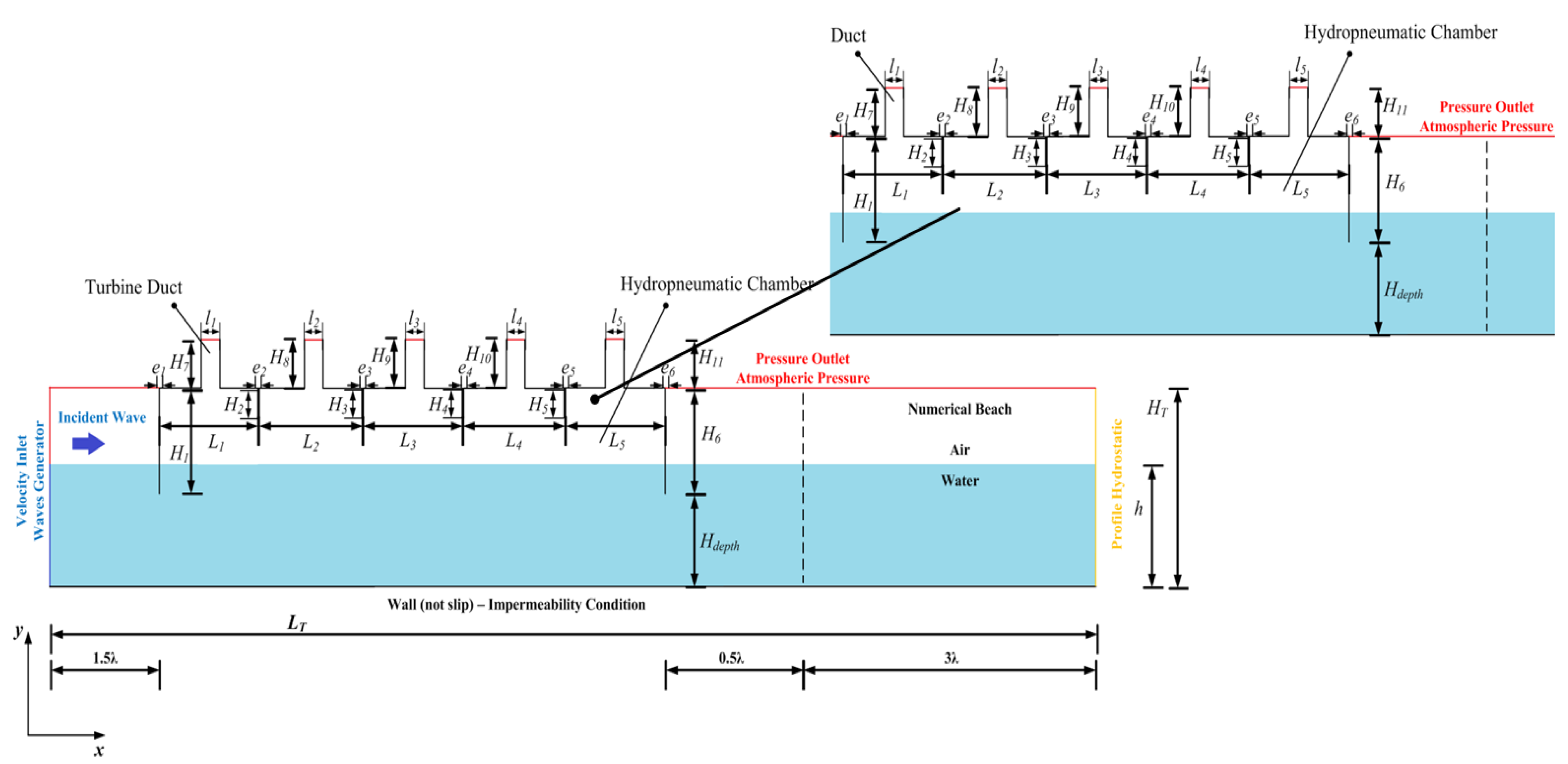
The dimensions of the numerical wave tank (see
Figure 3) depend directly on the wave characteristics adopted in the analysis. The depth of the water (
h) and the wave height (
H) (see
Figure 2) must be taken into account to determine the numerical wave tank height. This care is taken so that water does not occupy the space outside the computational domain. Thus, it is possible to define that the tank’s minimum height is given by
h + 3
H, as described in Gomes et al. [
18]. The wave considered in this work follows a real scale [
44].
The depth of wave propagation is the same as the wave tank. For the length of the tank, it is necessary to consider the wavelength (
λ). The tank’s dimensions and the waves’ characteristics are the same as presented in Lima et al. [
20] and can be seen in
Table 2.
The dimensions of the converter device are also defined and can be seen in
Figure 4, in detail, highlighting the height of the hydropneumatic chambers (
H1,
H2,
H3,
H4,
H5,
H6), the submersion depth of the device (
Hdepth), the heights of the turbine ducts (
H7,
H8,
H9,
H10,
H11), the length of the ducts (
l1,
l2,
l3,
l4,
l5), the length of the chambers (
L1,
L2,
L3,
L4,
L5), and the thickness of the columns that divide the devices (
e1,
e2,
e3,
e4,
e5,
e6).
3.3. Numerical Wave Generation and Boundary Conditions
The numerical wave generator is positioned to the left of the wave tank, as shown in
Figure 3 (highlighted in blue). The wave is generated using the methodology available in the software FLUENT
®, in which the used wave theory is defined (in the present work, it was 2nd-order Stokes), as well as the height and wavelength using the VOF methodology defined as the open channel wave boundary condition [
40]. The equation that describes the prescribed velocity boundary condition is defined by the following formulation, being divided into horizontal and vertical components [
22]:
The other boundary conditions are also shown in
Figure 3. The definition is the following: an atmospheric pressure condition (outlet pressure—lines in red color) is applied on the upper left side, as well as on the upper surface of the tank and at the outlets of the turbine ducts; the condition of non-slip and impermeability (wall—lines in black color) is applied on the bottom of the tank and the walls of the devices. The right surface has a hydrostatic profile (line in yellow color) to eliminate the reflection effect of the waves.
In addition to the boundary conditions, it is considered an initial fluid condition at rest (flat condition), with depth h = 10 m and t = 0 s in the free surface elevation equation (Equation (1)). This equation calculates the wave tank’s water elevation and determines the wave height at different locations.
A numerical beach region was inserted into the tank to decrease the wave reflection effects. A sink term (
S) is added to the momentum conservation equation, given by [
37,
45,
46]. An error is introduced with the addition of a term in the conservation equation. A more detailed study regarding its estimation with linear and quadratic terms analysis can be seen in [
47].
The mathematical formulation is presented in the following equation [
45,
46]:
where
C1 and
C2 are the linear and quadratic damping coefficients, respectively, the term
refers to density,
is the velocity, z is the vertical position,
zfs and
zb are the vertical positions of the free surface and bottom, respectively,
x is the horizontal position, and
xs and
xe are the horizontal positions of the beginning and finish of the numerical beach, respectively. According to Lisboa et al. [
48], it is recommended to assume
C1 = 20 and
C2 = 0.
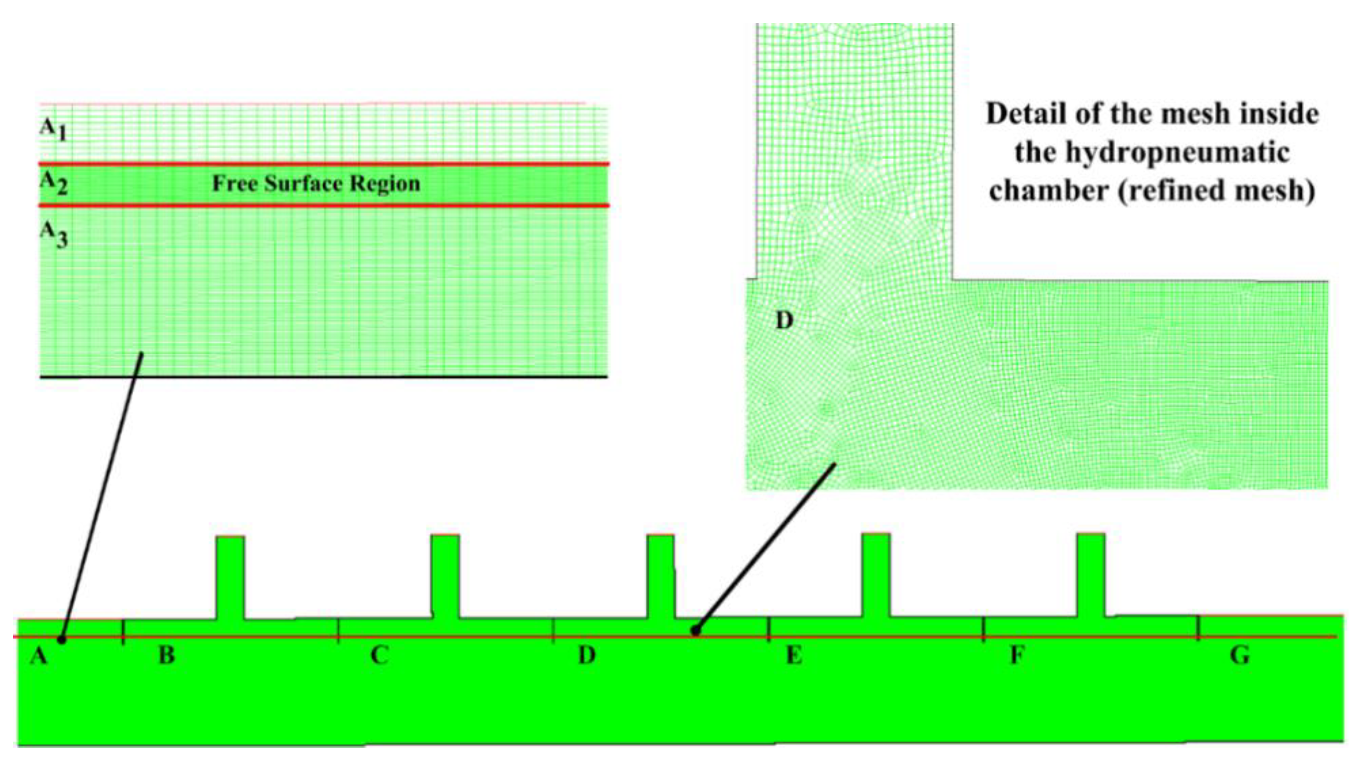
3.4. Computational Mesh
The discretization of the computational domain is performed with finite rectangular volumes. All computational meshes generated in the investigation followed the stretched methodology developed by Mavriplis [
49]. The application of this technique consists of defining regions more refined than other ones. These regions are defined through the investigation’s interest; they are the free surface regions in the present work.
Figure 5 shows the two-dimensional mesh for the case of five coupled chambers. The computational domain was divided into three regions: before the devices, inside, and after them. Region A represents the domain before the OWC devices and is divided vertically into three sub-regions to define one of them with greater refinement, as indicated by the stretched methodology: A
1, A
2, and A
3, and for the region of the free water surface (region A
2), a refinement of 40 volumes in the vertical direction and 120 volumes in the x-direction is adopted. Besides, 30 and 110 volumes are used in the vertical direction for the spatial discretization of regions A
1 and A
3, respectively, following the recommendations of Barreiros [
50]. In regions B, C, D, E, and F, there are the OWC devices, where one can check the most refined mesh inside them.
Squares of 0.1 m in length totaling 620 horizontal volumes were used for the devices’ region, while squares of 1 m in length were used for the regions outside the devices, as recommended by Gomes [
37]. The region G represents the geometry after the devices and has 200 horizontal volumes and the same vertical discretization of region A.
4. Constructal Design for Geometric Investigation of OWC
Constructal Design, the method used to apply the Constructal Law, allows obtaining better geometries by reducing its internal currents’ general resistance. The method relates degrees of freedom (geometric parameters that vary during the method execution processor), restrictions (parameters that are kept constant during the analysis of cases), and performance indicators (that must be improved, aiming to reach a superior performance) [
25,
51].
The method’s implementation scheme and all the steps necessary to execute it are presented in
Figure 6. All studied cases were analyzed based on the flowchart shown in
Figure 7. This scheme allows a better understanding of the studied cases and how they were considered the degrees of freedom. All analyzed geometries are shown in
Table A1,
Table A2 and
Table A3 located in the
Appendix A.
The studied geometries are presented below:
Table A1 presents the eleven geometric variations for each number of coupled chambers, where the variation in
n represents the number of coupled chambers.
Table A2 and
Table A3 present the study of the thickness and height of the walls that divide the coupled chambers for the case using five chambers. The present study assumed the geometry values with the highest performance of the hydropneumatic power performance indicator presented in the study by Lima et al. [
20].
The analysis of the different geometric configurations proposed is presented by evaluation of the Constructal Design Method results. The problem restrictions are the volume of hydropneumatic chambers (VEn), the total volumes (VTn), and device column thicknesses (en), where n varies from one to five, representing the number of coupled chambers.
Thicknesses are kept constant and equal to 0.1 m, as recommended by Lima et al. [
52]. As the chambers have the same geometry, the generalized formulation is defined, and the sub-index
n is used as the previous formulations, and
j varies from seven to eleven, representing the turbine ducts.
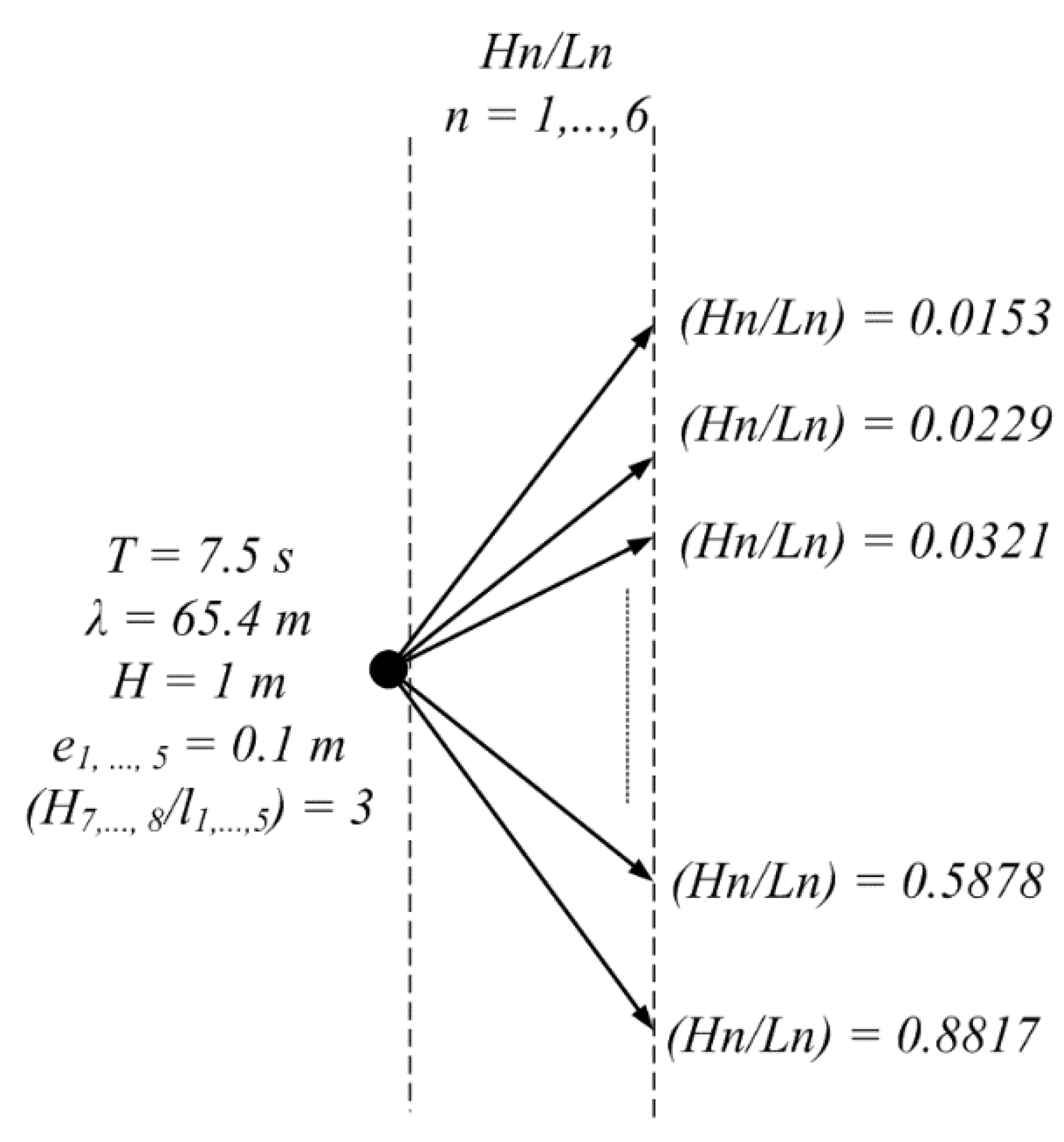
The dimension
W in Equations (10) and (11) is kept constant and equal to 1 m because it is a two-dimensional computational model. It is also considered an average characteristic of a real wave spectrum with a period of 7.5 s and a wavelength of 65.4 m. These values are defined according to the peak spectrum presented by Gomes et al. [
53].
The analyzed degrees of freedom of the work are the ratios between height and width of the hydropneumatic chambers (
H1/L1,
H2/L2,
H3/L3,
H4/L4, and
H5/L5). The volumes are defined in the following way:
VEn represents 70% of
VTn, and the same goes for the other incoming volumes, i.e.,
VTn = 93.4 m³ and
VEn = 65.4 m³. These values are defined based on the characteristics of the wave studied in the present work, beginning the first case with a length (
Ln) equal to the wavelength and height (
Hn) equal to the height of the wave. Through the previous equations, it is possible to determine the equations that define the lengths (
L1,
L2,
L3,
L4,
L5) and the heights (
H1,
H2,
H3,
H4,
H5,
H6) of the problem:
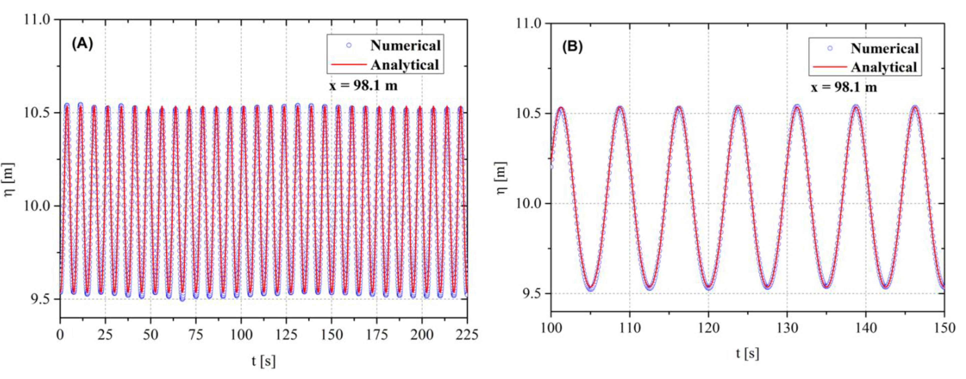
5. Verification and Validation of the Numerical Model
One way to evaluate the generated numerical waves is to compare the numerical free surface’s transient elevation with the respective analytical solution presented in Equation (1), maintaining the same position.
Figure 8 compares these results on a two-dimensional wave channel without the OWC device. The measurement probes are placed at
x = 98.1 m.
The total simulation time to perform the verification is 225 s, where
Figure 8A compares the results.
Figure 8B shows a time interval in which it is possible to observe small differences between the numerical and analytical data. The absolute difference between the solutions is measured instantly by calculating the error. Thus, the average of the differences is 1.48%, with the maximum value reaching 5.44%. These results show the accuracy of the numerical model used.
Validation of the numerical model considering the device is also required. The data obtained were compared with experimental and numerical results from Liu et al. [
11]. Thus, the dimensions of the wave channel and the OWC device are described in Liu et al. [
11] and determine a computational domain. In all cases, the turbine is not inserted into the turbine duct, and air pressure and air velocity variations are analyzed in the hydropneumatic chamber for the different wave periods mentioned above. Thus, the results were compared with those obtained numerically and experimentally by Liu et al. [
11].
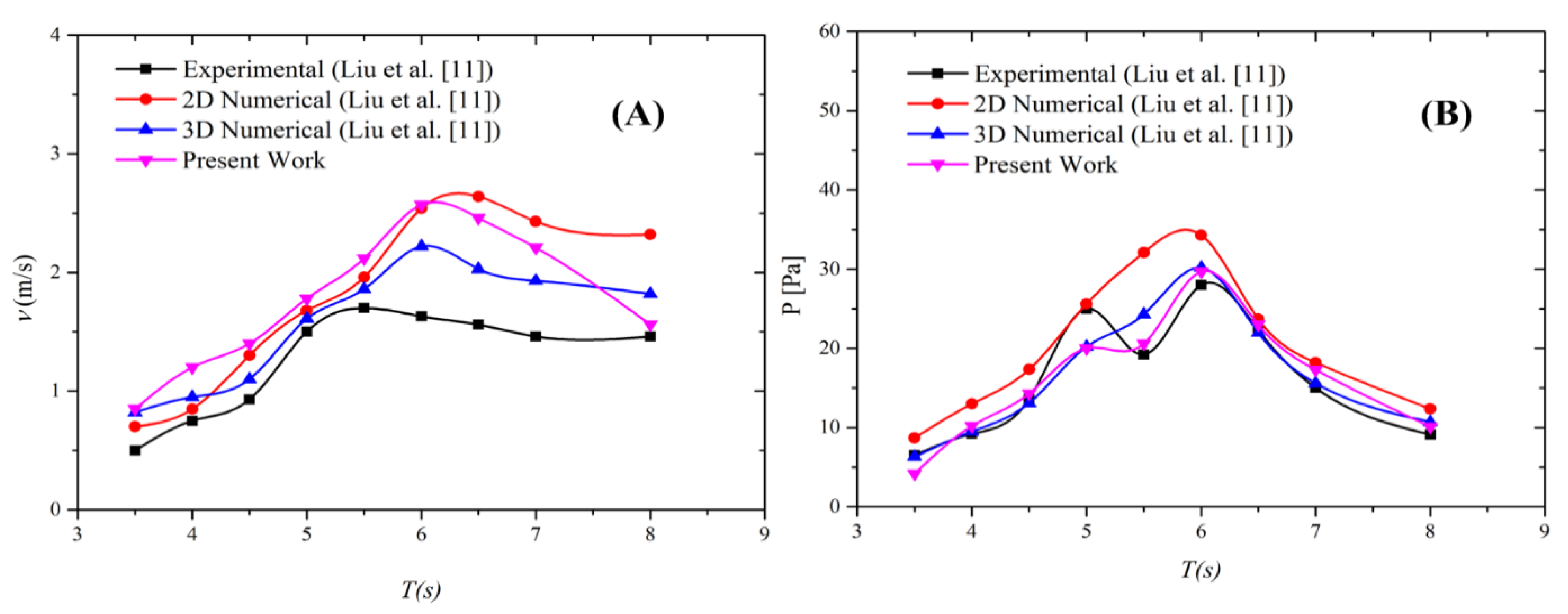
It should be noted that the numerical model adopted here differs from the numerical model employed by Liu et al. [
11] because when comparing the discrete results obtained for velocity, they are overestimated regarding the magnitudes of the experimental velocities; this fact is justified due to the resonance effects between the waves and chamber. The numerical values obtained agree with those in the previous works considering 2D and 3D domains, as shown in
Figure 9A.
Despite the differences in the results, both the velocity and pressure magnitudes are in line with the numerical results of the reference and, mainly, with the experimental results for the pressure field in
Figure 9B. It can be noted that as the period (
T) of the waves increases, the relative pressure also increases: for
T = 6.5 s and 7 s, the obtained results are between the 2D and 3D results of Liu et al. [
11], while for
T = 8 s, the proposed computational model conducts to practically the same value of the experimental result.
The mathematical and numerical model used in this work considers the flow in a laminar and incompressible regime, these being one of the simplifications of the real model adopted. As shown by Liu et al. [
11], in the inner region of the chamber, the number of calculated Reynolds is high, thus configuring a turbulent flow and using a Reynolds-averaged Navier–Stokes (RANS) approach with the standard k-ε turbulence model.
Although the results obtained in the present work are not fully convergent with those presented by Liu et al. [
11], in general, they have the same trends as the numerical and experimental results of the authors. Therefore, it is possible to consider the employed computational model as verified and validated.
6. Results and Discussion
The current investigation’s main purpose is to maximize the available hydropneumatic power of the OWC device, which depends directly on the pressure and mass flow rate changes due to the proposed geometric variations of the hydropneumatic chamber. The RMS (root mean square) was used to calculate the average values of the performance indicator. The monitoring of the water-free surface elevation takes place through the following integral:
where
αwater is the amount of water in each volume and
At is the area of each volume (m²). The following integral is used to monitor the mass flow rate in the center of each turbine duct:
where
represents the air velocity in the z-direction (m/s), and
ρair is the density of the air (kg/m³). The mean values were calculated using the arithmetic mean for transient RMS problems:
where
n represents the quantity to be calculated on the average RMS. For further details, it is recommended to consult Marjani et al. [
54].
The available hydropneumatic power is calculated according to [
55]:
where
pe,air is the static pressure in the turbine duct of the OWC device (Pa),
is the air mass flow rate through the turbine duct (kg/s), and
vair is the velocity of the air in the turbine duct (m/s); the other parameters can be found in Gomes [
37] and Lima [
56].
Altogether, seventy-six different geometric configurations proposed by the Constructal Design application are analyzed in relation to the height and length of the devices, keeping the input volume constant. The choice of values is made considering the height of the wave tank so that the height of the devices does not reach the bottom of the tank, making the passage of water impossible and its length not being so small as to make the energy conversion unviable. The cases of geometric variation in the thickness and height of the wall dividing the devices can be found in Lima et al. [
20].
The numerical simulation process starts with an OWC device with only a single hydropneumatic chamber and analyzes pressure, mass flow, and hydropneumatic power as the degrees of freedom vary. This process is repeated with the increase in coupled chambers up to a total of five.
The analysis of the results takes place by exploring each chamber individually and, thus, defining the highest values for the performance indicators. The result obtained in each chamber is added to the others in the coupled cases. The maximum performance of the device is defined as the sum of the individual performance indicators of each one.
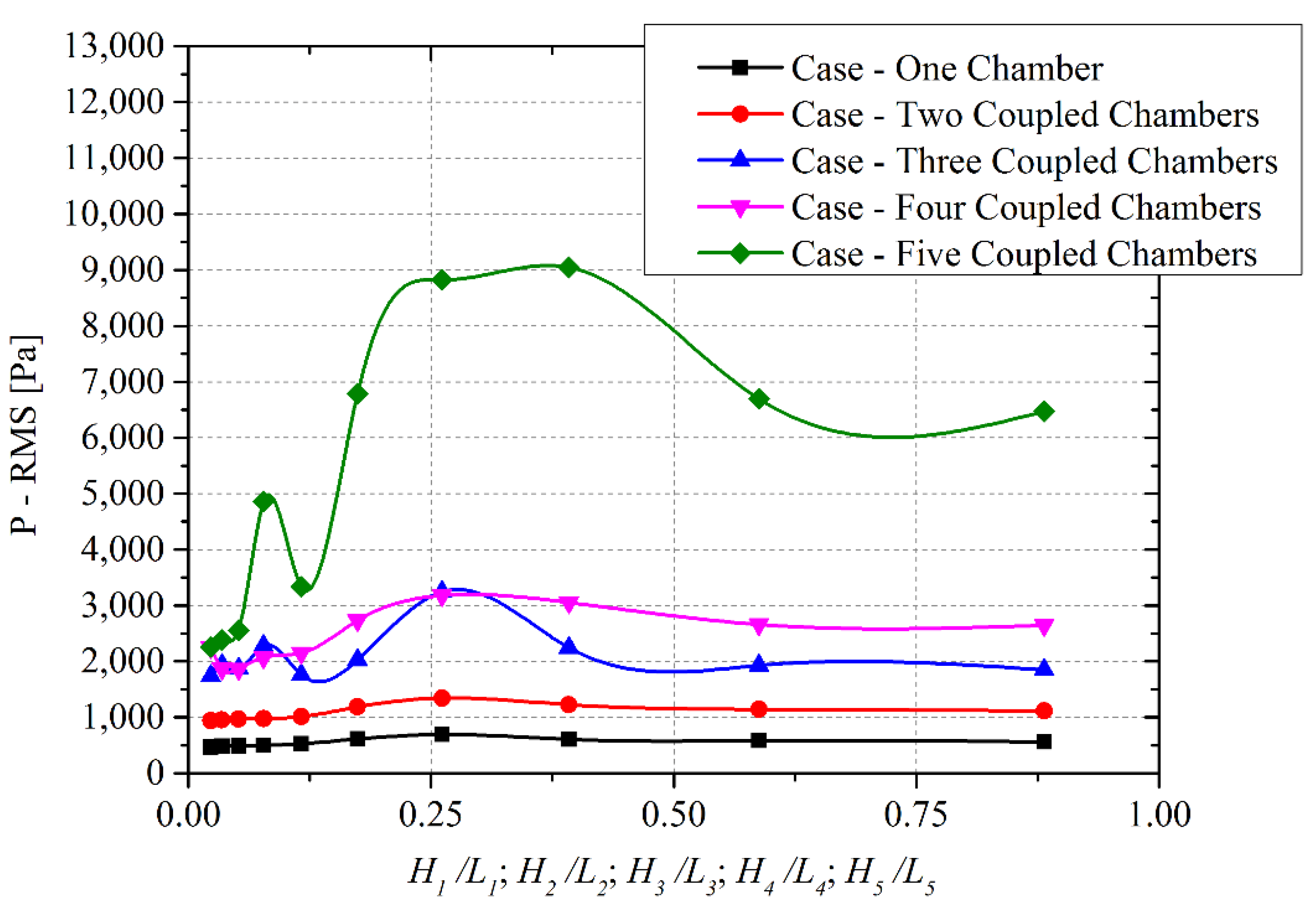
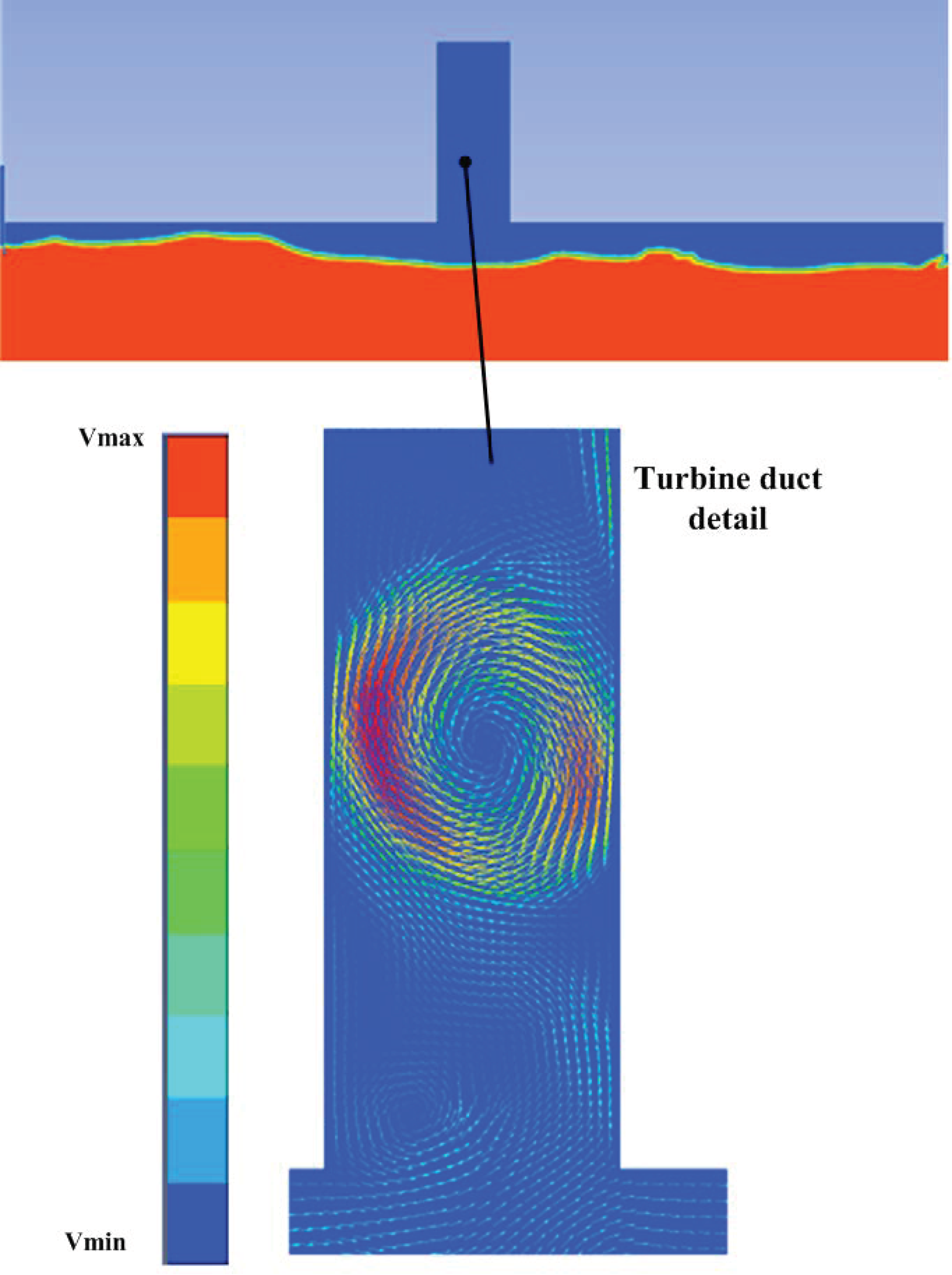
Figure 10 shows the RMS pressure values for the cases varying the number of coupled chambers (CC), where each line represents each of the studied cases. The increase in pressure occurs for two reasons. The first is that with the increase in the CC height, there is a greater pressure concentration in each chamber, even with the increase in CC. The second reason refers to the geometry of the chambers. It appears that the chambers with three coupled devices present a higher pressure than chambers with four devices in some configurations.
This behavior is due to the reflection of the waves inside the chambers, making the oscillatory movement more discontinuous and increasing the piston effect, consequently increasing the pressure and velocity, causing recirculation in the turbine duct, as can be seen in
Figure 11, with the detail of one of the chambers and its turbine duct. The interval with values of 0.25 <
Hn/Ln < 0.50, for the five cases analyzed, presents in all of them its highest pressure values.
It is understood that these geometric configurations within this range provide an increase in the accumulated pressure due to the decrease in the entrance length of the devices and an increase in the height. The simulation of the piston movement caused by the compression and decompression of the chamber with a greater vertical path to move shows the growth of the internal pressure in all chambers, directly influencing the hydropneumatic power.
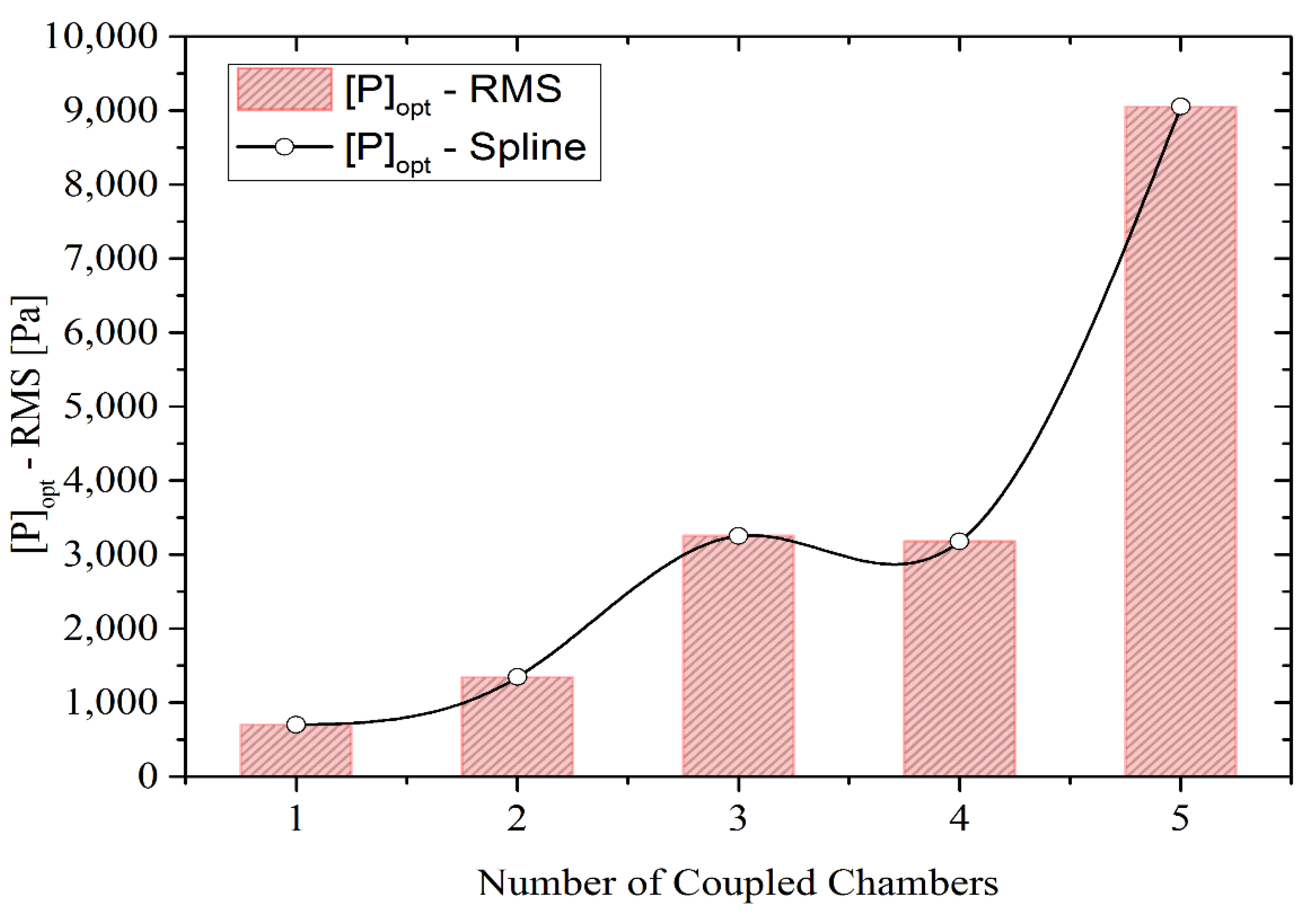
Figure 12 shows the highest values of accumulated pressure for each case studied, remembering that for each geometric configuration analyzed, the pressure in each coupled chamber is added, being its total the accumulated pressure. In this figure, it is possible to identify that devices with only one chamber have lower pressure values than the others, and this behavior can be explained by the low accumulated pressure that occurs due to having a single chamber.
Note that devices with three chambers have higher pressure values than devices with four chambers. This behavior is due to the more regular piston effect in devices with three chambers coupled. Devices with five coupled chambers have the highest accumulated pressure value, and the cases with the highest performance in all analyzed geometries are also concentrated in the same range of values.
It can be noticed that devices with a greater number of coupled chambers present higher pressure, a parameter that directly implies the calculation of the hydropneumatic power, as can be seen in Equation (19). Besides, there is a pattern and tendency to increase pressure with an increase in hydropneumatic chambers.
The mass flow rate is another component for the calculation of the hydropneumatic power equation. It directly influences the calculation and, through the airflow that passes through the turbine duct, energy conversion occurs when there is an implanted turbine.
Figure 13 shows the behavior of the mass flow rate for five related studies. As well as pressure, the highest performance cases are within the same range of values for the cases analyzed (0.25 <
Hn/Ln < 0.50). The justification for this conclusion is through the compression and decompression process, which, like pressure, occurs with an increase in the height of the chambers and a decrease in width, keeping the inlet volume fixed.
There is a gradual and uniform increase in all cases, with a peak value for the performance indicator at the same point of Hn/Ln in all analyses. As the ratio increases, that is, the chamber height increases and the length of the chamber decreases, there is a decline in the mass flow rate values. This behavior is justified by the length of the duct in which the device’s turbine is located, which remains constant because even with high pressure, the mass flow rate tends to decrease.
As in the pressure, after analyzing the RMS of the five geometric configurations, the values with the highest mass flow rate are checked and the development of these values is studied with the increase in the number of coupled chambers, as seen in
Figure 14. As the number of coupled chambers increases, the mass flow rate also increases. This phenomenon explains the more significant number of piston effects in the hydropneumatic chambers and the increase in mass flow rate. In all cases, the length and height of the duct would have the same values in the energy conversion turbine.
The hydropneumatic power represents an association of the results obtained with the mass flow and pressure, as shown in Equation (19).
Figure 15 shows the variation of the accumulated hydropneumatic power for all studied cases. With the increase in the number of coupled devices, there is an increase in hydropneumatic power. This fact can be explained due to the rise in pressure and the accumulated mass flow as the number of coupled chambers increases.
As in the other analyzed quantities, the available hydropneumatic power presents its highest values in each of the configurations studied in the range of 0.25 < Hn/Ln < 0.50. The increase in the power indicates that more energy is being converted into the device, so with five chambers coupled, the maximum accumulated hydropneumatic power is greater than the other cases. In addition, the hydropneumatic power shows a maximum point, but after it starts to decrease. This behavior is due to the hydropneumatic chamber’s geometry. With the increase in the chamber, the greater its height and the smaller its length, and the lesser energy is converted.
Figure 16 shows the results of the highest accumulated hydropneumatic power for all cases. When comparing the cases of three and four CC, it is possible to identify a slight power difference noticeable that the case with three CC of higher performance presents a greater accumulated power than the case with four chambers.
The results of
Figure 16 show that the addition of five coupled devices converts more hydropneumatic power than the other cases with a lower number of coupled chambers. The geometric analysis of the structure determines the configuration that presents the maximum hydropneumatic power converted for all the analyzed cases. It is a helpful tool in construction projects of devices converting the energy of the sea waves in the function of its large structures.
Using the Constructal Design method associated with the exhaustive search method was decisive for analyzing the data. The geometric variation defined through the method and the analysis of degrees of freedom and performance indicator results showed the available power converted when only cases ranging from one to five coupled hydropneumatic chambers were analyzed.
The case with the highest performance within the displayed range, with five chambers coupled and geometry with the ratio Hn/Ln = 0.2613 (Hn = 4.1335 m and Ln = 15.8219 m), led to a hydropneumatic power of [Phyd]opt = 30.8 kW. The lowest performance case has one chamber, and the ratio Hn/Ln = 0.2613 (Hn = 4.1335 m and Ln = 15.8219 m) conducting to a hydrodynamic power of [Phyd]opt = 200 W.
Another aspect obtained through the results presented is a theoretical recommendation using the parameters height and wavelength referenced in the numerical investigation.
The geometric configurations that present the maximum conversion are within the range 16 (H/λ) < Hn/Ln < 32 (H/λ). This range is the theoretical recommendation for the cases of coupled devices, based on the interval that led to the highest performance for each number of coupled devices (0.25 < Hn/Ln < 0.50). Thus, the Constructal Design method associated with the exhaustive search optimization method proves to be a handy tool for analyzing devices with multiple coupled chambers and understanding the effect of design and the number of chambers on device performance.
7. Conclusions
The present work carried out a numerical study of an OWC wave energy converter, considering different numbers of coupled devices. The objective of the investigation was to evaluate the influence of the geometric variation and the number of coupled hydropneumatic chambers, keeping the volume of the device constant over the available hydropneumatic power converted by the devices.
The studies carried out applied the association of computational modeling with Constructal Design and Exhaustive Search. The first is based on CFD, which approaches the mass and momentum conservation equations in differential form through a system of algebraic equations and uses the VOF methodology, which reproduces the interaction between the fluids involved in the numerical simulation. The exhaustive search method allows one to go through all the results and discover the geometric arrangement with the highest performance of each coupled chamber number into the search space defined with Constructal Design.
As part of the Constructal Design method, degrees of freedom were defined as H1/L1, H2/L2, H3/L3, H4/L4, and H5/L5. The problem restrictions in question were defined as the volume of the hydropneumatic chambers (VE1, VE2, VE3, VE4, and VE5), the volume of each hydropneumatic chamber added to the turbine duct volume (VT1, VT2, VT3, VT4, and VT5), and the thickness of the columns that divide the devices, which are kept constant (e1, e2, e3, e4, and e5).
The results for pressure, mass flow rate, and available hydropneumatic power were analyzed. All the results were presented for each of the studied geometries. The dimension variations of the hydropneumatic chambers are responsible for the increase or the decrease in pressure and mass flow rate, also associated with the oscillatory movement of the waves inside the chambers, thus creating the piston effect that varies along with the geometries.
The pressure and mass flow rate have an important influence on the estimate of hydropneumatic power. This aspect can be attested by the range of geometric ratios in which the highest performance cases are the same for the three parameters. In all configurations of coupled chambers, a maximum point was verified in the power results. These results show the tendency to achieve one point of optimal performance of the length/height ratio of the hydropneumatic chamber.
The results show that as the number of chambers increases, the performance indicator has higher values for the present conditions studied. Therefore, devices with five coupled chambers led to the highest magnitudes of hydropneumatic power. In all cases analyzed, the optimal values were always in the range 0.25 <
Hn/
Ln < 0.50. For a lower number of coupled chambers, these magnitudes of the ratio Hn/Ln were in the same range reached by other authors, e.g., Lima et al. [
19,
20]. The difference of the available hydropneumatic power for the optimal and worst cases, within the range of values
Hn/Ln investigated, was 85.4%. The geometries and powers of these cases show that
Hn/Ln = 0.2613 (
Hn = 4.1335 m and
Ln = 15.8219 m),
[Phyd]opt = 30.8 kW and
[Phyd]opt = 4.5 kW for the higher and lower hydropneumatic power, respectively.
Thus, it is inferred that with the analysis of the insertion of hydropneumatic chambers, keeping the input volume constant, devices with five chambers coupled have an increase in the energy conversion superior to the other cases with fewer chambers. Future work must analyze the variation in degrees of freedom involving the turbine ducts and thus determine the complete geometric configuration (hydropneumatic chamber plus turbine duct) that conducts the highest hydropneumatic power.


 ,
, 

