Abstract
We demonstrated the relationships between elemental carbon (EC) and EC fractions during evolved gas analysis (EGA) for PM2.5 sampled at KOREATECH from 29 March 2018 to 12 May 2018. The EC concentrations were compared to the concentrations of equivalent black carbon to confirm that the level of EC concentrations analyzed in this study was valid. Among various EC fractions and their combination, EC1+EC3 fractions were best correlated with the EC concentrations. Especially, dominant EC fraction was related with the dependence of carbon oxidation quantity on the oxidation temperature. We also examined the relationships between pyrolytic carbon (PyC) and EC concentration with respect to the split time. PyC was correlated with the split time in the phase of oxygen-helium mixture. PyC was close to zero for the split time in the helium phase. It is novel, as far as the authors know, that the correlation between PyC and the split time under NIOSH 5040 protocol was reported with regard to EGA. We believe that our study helps to identify what causes uncertainty in the quantification of PyC.
1. Introduction
Particulate matter (PM) which is composed of carbonaceous aerosols, ions, and elemental components affects not only human health but also climate change [1,2,3,4,5,6]. Carbonaceous aerosols such as organic carbon (OC) and elemental carbon (EC) have been measured and quantified by an evolved gas analysis (EGA) among various analytic methods [7,8,9,10,11]. Thermal-optical analysis, one of the EGA methods, uses different responses of light-absorbing carbonaceous aerosols to the temperatures of collected samples. The sample is analyzed in a helium (He) phase and a helium-oxygen (He-Ox) phase. In the He phase, the OC components collected on the filter are volatilized by increasing the temperature step by step under a helium atmosphere. In the next phase (He-Ox phase), the EC on the filter is oxidized at various temperatures with helium-oxygen mixture. The OC and EC components volatized from the filter are oxidized to carbon dioxide and then reduced to methane. Eventually, the reduced methane concentration is measured to quantify the amount of OC and EC. OC is mostly measured by volatilization from the filter at the He phase, but some of the OC is carbonized or pyrolyzed. Then, they remain volatile on the filter. This is called as the pyrolyzed carbon or pyrolytic carbon (PyC), which absorbs light as EC does. Usually, PyC is oxidized in the He-Ox phase and is recognized as if it were EC. Therefore, it is important to carefully calculate PyC for better quantification of OC and EC. The optical attenuation measurement is commonly used to determine PyC. The intensity of transmitted or reflected light is continuously monitored during analysis, in which the intensity decreases by the PyC and then increases by the oxidation of PyC again. The point at which the intensity of transmitted or reflected light becomes equal to the intensity at the start of analysis is defined as the split time. PyC is artificially calculated from the EC fractions from the beginning of the He-Ox phase to the split point. The measurement of OC and EC depends on analysis protocols in which the temperature profiles and the thermal decomposition correction methods are defined in different ways from each other. The analysis protocols include Interagency Monitoring of Protected Visual Environment (IMPROVE), National Institute for Occupational Safety and Health (NIOSH 5040), European Supersites for Atmospheric Aerosol Research (EUSAAR) and Specification Trans Network (STN), a modification of NIOSH temperature protocols [10,11,12,13]. Each protocol has a different operating temperature profile as shown in Table 1.

Table 1.
Details of various protocols for OC/EC analysis [10,11,13,14,15].
Equivalent black carbon (eBC) concentration is usually measured by filter-based optical transmittance instruments such as an aethalometer, and its limitation has been updated [14]. A multi-angle absorption photometer (MAAP), another filter-based instrument, was successfully applied to the continuous monitoring of local eBC concentrations for more than three months [16,17]. Thus, we employed the MAAP in order to verify EC concentrations with the help of eBC concentrations.
PyC complicates the quantification of EC. The split time is associated with the determination of PyC quantity. This study aims to find not only a relationship between EC and various EC fractions but also the role of PyC in quantifying EC. Uncertainties have been reported on the analysis of OC and EC. For example, PyC depended on how to define the split time and on data processing in the analyzer [18]. Another example is that metal salts might affect the quantification of OC and EC in the case of diesel exhaust particles [19]. However, efforts are underway to quantify OC and EC using a thermal-optical transmittance or a thermal-optical-reflectance despite such uncertainties.
In order to better understand EC quantification, we have just initiated the investigation of PyC, the split time, EC concentration and their relationships. First, the relationship between various EC fractions vs. EC will be examined to confirm which EC fraction dominates EC concentration. Second, the EC concentration will be compared with the eBC concentration for verification purposes. Third, the PyC, the EC concentration, the split time and their relationships will be presented to find the role of the split time in quantifying PyC.
2. Materials and Methods
2.1. Sampling of PM2.5
Samples of atmospheric aerosols were collected from 29 March 2018 to 12 May 2018 at every 8 h by a low-volume sampler (PMS-104, APM, Bucheon, South Korea). A PM2.5 WINS impactor was installed at the inlet of the low-volume sampler to cut off particles larger than 2.5 μm. Sampling site is located at Korea University of Technology and Education (KOREATECH) Byeongcheon Campus (36.765° N, 127.280° E, about 15 m high from the ground) which lies in the middle of South Korea as shown in Figure 1. Atmospheric aerosols were collected on 47 mm Whatman Quartz fiber filters (QM/A, Whatman Inc., Maidstone, UK) which had been baked at 600 °C for 4 h in an electric furnace before sampling.
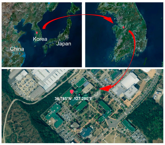
Figure 1.
Location of sampling site at KOREATECH Byeongcheon Campus (36.765° N, 127.280° E).
2.2. eBC Measurement
The eBC mass concentration was continuously measured with a MAAP (MAAP 5012, Thermo Scientific, Waltham, MA, USA). Attenuation through a filter tape was measured together with scattering intensities at two different positions. Multiple scattering effects were compensated for attenuation and it was converted into eBC concentration. A PM2.5 WINS impactor was also installed at the inlet of our MAAP.
2.3. EC Measurement
An OC/EC Analyzer® (Sunset Laboratory Inc., Tigard, OR, USA) was used to measure atmospheric EC concentrations and showed information about masses of EC1, EC2, EC3, EC4, EC5 and EC6 which are EC fractions at each temperature profiles applied.
OC and EC were quantified for 1.5 cm2 punches of the quartz filter samples using a thermo-optical evolved gas analysis under NIOSH 5040 procedure [10,20]. Carbon deposited on the filter was oxidized to carbon dioxide, and then reduced to methane for detection with a flame ionization detector (FID) [19]. A laser (wavelength 670 nm) was used to monitor transmittance through the filter [19]. The split time was set as the time at which the transmittance returns to its initial value [19]. As shown in Table 1, most volatilized carbon evolves in the He phase while the temperature is heated stepwise to 310 °C for 80 s, 475 °C for 80 s, 615 °C for 80 s and 870 °C for 110 s, being analyzed into four OC fractions. The 98% He/2% O2 atmosphere is introduced after the oven cools to 550 °C, and the oxidized carbon evolves at 550 °C for 45 s, 625 °C for 45 s, 700 °C for 45 s, 775 °C for 45 s, 850 °C for 45 s and 870 °C for 110 s, being analyzed into six EC fractions, EC1, EC2, EC3, EC4, EC5 and EC6, respectively [19]. The carbon that evolves in the oxidizing atmosphere until the transmitted light returns to its initial value is termed as PyC, which is subtracted from the sum of EC fractions to obtain the EC concentration [19]. In other words, EC mass is calculated by the sum of EC1, EC2, EC3, EC4, EC5 and EC6 minus PyC.
3. Results and Discussion
3.1. Oxidation Quantity vs. Oxidation Temperature
A typical example of the protocol with thermogram used in our study is shown in Figure 2a. Changes in FID signals, transmittance, absorbance and temperature are relatively indicated and one can see that a split point is located between EC1 and EC2 fractions. The curve in Figure 2b was adopted from another study [21] in order to explain the oxidation quantity of carbon graphite contents increased with temperature. At low temperatures, between 400 °C and 500 °C, the oxidation quantity is very small, while the oxidation quantity increases from 500 °C to 800 °C, where EC1, EC2, EC3 and EC4 are quantified as shown in Figure 2a,b. EC losses may be more pronounced with NIOSH type protocols because the temperature of the inert He phase is higher than IMPROVE as can be seen in Table 1. OC and EC concentrations are affected by temperature profiles. For example, EC concentrations analyzed using IMPROVE were larger than those analyzed using NIOSH 5040 [22]. Particularly in He-Ox phase, the temperature profiles of IMPROVE is different from that of NIOSH 5040. The EC concentrations would result in larger values if IMPROVE protocol were employed in this study.
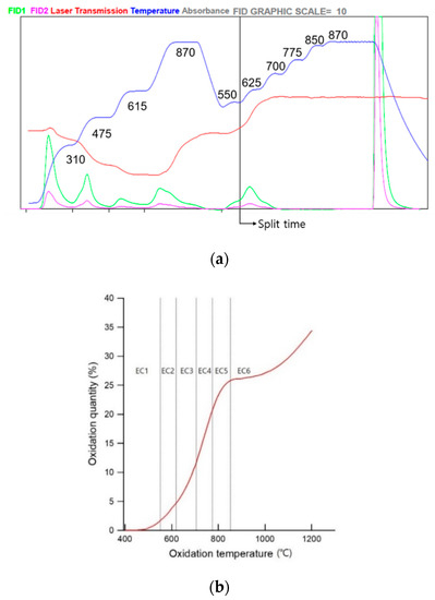
Figure 2.
(a) An example of relative profiles of temperature, transmittance, absorbance and FID signals used in this study; (b) Carbon oxidation quantity as a function of temperature. The curve was adopted from another study [21].
Reducing the temperature of inert He phase may minimize split time issues, although OC does not completely evolve sometimes. It is difficult to determine which protocol is proper to quantify OC and EC because there is no standard reference materials for EC.
3.2. Comparison of EC with eBC
Figure 3 shows time series of eBC and EC concentrations. Blue line represents eBC concentrations measured every minute and averaged with 8 h for comparison with better display. Red circles represent EC concentrations of samples collected every 8 h as explained earlier. The average of eBC concentrations was 1.23 μg/m3, and the average of EC concentrations was also 1.23 μg/m3. The level of EC and eBC concentrations was similar to the average eBC concentration measured by our group [17]. Thus, the EC and eBC concentrations are comparable. EC concentrations are in good agreement with eBC concentrations despite fundamental differences between the thermal-optical technique and the filter-based light attenuation technique. Intermittent breaks in EC measurements stemmed from the failure of the automatic low-volume sampler caused by malfunction of an internal vacuum pump.
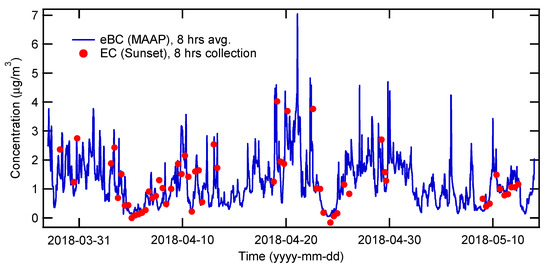
Figure 3.
Time series of comparison plot between EC and eBC concentrations.
3.3. Various EC Fractions
Figure 4 shows EC concentrations together with each EC fraction from EC1 to EC6. The black bars represent EC concentrations. EC1 to EC6 fractions are shown as red, blue, green, sky blue, white and yellow bars, respectively. When the sum from EC1 to EC6 is larger than EC, it is regarded as being overestimated than the actual amount of EC collected by the analysis process. The difference between EC and the sum from EC1 to EC6 is calculated to be PyC as explained earlier. As a matter of fact, PyC was observed to be sometimes prominent as can be seen in Figure 4. PyC values sometimes reached up to 50% of the sum from EC1 to EC6 fractions. However, the high PyC values were not unreasonable because the EC concentration was similar to eBC concentration measured when PyC was high. In this study, the dominant fractions of the EC turned out to be EC1, EC2 and EC3, which implies that carbon was oxidized mostly at relatively low temperature. Ambient organic aerosols may exist as highly viscous semi-solids or amorphous glassy solids [23]. High viscous state can result in the decrease in diffusion as can be inferred from the Stokes–Einstein equation, so that diffusional mixing can subdue. The suppressed diffusion can prevent the oxygen from contacting with the EC on filter. This is valid in ambient temperature range. Once the ambient organic aerosols are introduced into the analyzer, the temperature surrounding the aerosols increases to 310 °C at OC1 step in He phase, and further increases up to 870 °C at EC6 step in He-Ox phase. In these temperature ranges, most of the ambient organic aerosols are prone to be vaporized or volatilized. The viscosity of gaseous organic compounds increases as temperature increases. Consequently, the high viscous state may cause the inhibition of the oxygen from touching the EC at some high temperatures, for example, 850 °C in EC5 step, and 775 °C in EC4 step. This is why EC4 and EC5 fractions turned out to be minor fractions in this study. EC6 fractions outstood intermittently during the measurement period. The EC6 fraction is calculated from the area of FID signal, where the oven temperature is maintained at 870 °C. This means that some portion of carbon fraction was reluctant to react with oxygen at some temperatures, but rather was oxidized at 870 °C. EC6 was excluded in the comparison study. Thus, we considered only EC1, EC2 and EC3 for comparison as follows.
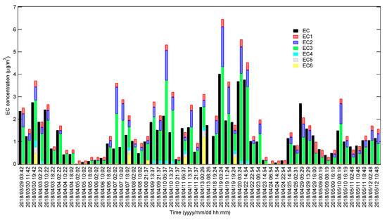
Figure 4.
EC concentrations and EC fractions obtained through EGA in this study.
Figure 5 shows the correlation of EC fractions and their combinations with the EC mass concentration. It was possible to determine a dominant EC fraction in EC mass concentration. As shown in Figure 5a, EC1, EC2 and EC3 concentrations versus EC mass concentration together with linear regression fitting curves demonstrated the contribution of individual EC fraction to EC. Figure 5b presents EC1 + EC2 concentrations versus EC mass concentration, which show the effect of the carbon oxidation at relatively low temperature. Figure 5c shows EC1 + EC3 concentrations versus EC mass concentration. Figure 5d shows EC2 + EC3 concentrations versus EC mass concentration. Figure 5e shows EC1 + EC2 + EC3 concentrations versus EC mass concentration. The slope, y-intercept, their standard deviations and R2 of each graph are shown in Table 2. The slope of linear fitting curve of EC1 versus EC was the lowest, which implies that EC1 contributed to EC less than EC2 and EC3 did. Among EC1, EC2 and EC3, the slope of linear fitting curve of EC3 versus EC was the highest and R2 of EC3 versus EC was the highest, too. Therefore, EC3 turned out to be the dominant fraction for the quantification of EC in the present study. As can be seen in Figure 5b–d and Table 2, EC1 + EC3 versus EC exhibited the highest correlation, while EC1 + EC2 versus EC showed the lowest correlation. The slope of the linear fitting curve of EC1 + EC2 + EC3 versus EC was larger than 1 as can be seen in Figure 5e and Table 2. This implies that EC1 + EC2 + EC3 was overestimated in comparison with EC. The comparison result on the correlations of EC fractions and their combinations with EC mass concentrations suggests that EC3 is the most dominant fraction to compose EC mass concentration. That is, EC3 is the most ‘appropriately’ correlated with EC as a single fraction, and is oxidized to CO2 at 700 °C. EC1 + EC3, among others, as a combination of multiple fractions is the ‘best’ correlated with EC.
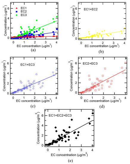
Figure 5.
The relationship between EC fractions and EC concentration: (a) EC1 vs. EC, EC2 vs. EC and EC3 vs. EC; (b) EC1 + EC2 vs. EC; (c) EC1 + EC3 vs. EC; (d) EC2 + EC3 vs. EC; (e) EC1 + EC2 + EC3 vs. EC.
Table 2.
Summary of linear regression on the EC fractions and their combination versus EC concentrations.
3.4. PyC, Split Time and EC Concentration
PyC can be formed due to various reasons. PyC is present mainly in the He-Ox phase, where, pre-oxygen (Pre-Ox) split time is defined. In this study, the Pre-Ox split time ranged from 330 s to 390 s. PyC may be exceptionally created in the He phase. There are several reasons why PyC is created in the He phase. Oxygen may leak in the He phase due to electrical issues or the malfunction of sensors installed in the OC/EC analyzer. Loose fitting of connectors and extremely small amount of oxygen in the helium gas are potential causes of Pre-Ox split time that may constantly provide oxygen to a sample cell during the He phase and consequently are regarded as instrument-specific issues [24]. Another reason may be that the presence of metal salts in the samples caused the Pre-Ox split time issue. It was reported that metal salts reduced the temperature required to make EC [19]. Thus, metal salts may enhance the charring of OC. Post-oxygen (Post-Ox) split time ranged from 440 s to 500 s in this study, where 2% of oxygen is included in the He base environment. No split time is defined between 390 s and 440 s because the He phase is changed into the He-Ox phase. It is interesting to note that negative PyC exists sometimes. Figure 6a shows the split times at various EC concentrations. When EC concentration was higher than 3 μg/m3, only Post-Ox split times were present. When EC concentration was lower than 3 μg/m3, however, Pre-Ox split times were present together with Post-Ox split times between 300 s to 500 s. In addition, Pre-Ox split times were clearly separated with Post-Ox split times due to mode change from He phase to He-Ox phase. In Figure 6b, PyC is plotted as a function of split time. As for Pre-Ox split times, PyC was nearly zero or negative. As for Post-Ox split times, however, PyC showed non-zero values at high split times. This trend was observed in the other study [25]. Figure 6c shows that negative PyC was observed at EC concentration lower than 3 μg/m3. This is reasonable because negative PyC can be observed only at Pre-Ox split times and Pre-Ox split times are present only for EC concentration lower than 3 μg/m3 in the present study as shown in Figure 6a. Split time of 360 s corresponds to Pre-Ox split time and only OC is involved in the analysis of carbonaceous aerosols. In contrast, 450 s and 495 s are involved in the analysis of EC1 and EC2, respectively. The amount of carbon oxidation in EC1 and EC2 states are small as inferred from Figure 2b. Therefore, EC1 and EC2 did not contribute to EC concentration much. However, it is obvious that the amount of carbon oxidation in EC3 is larger than those in EC1 and EC2 as can be seen in Figure 2b. It is noted that the oxidation quantity is dramatically increased at 700 °C as shown in Figure 2b. This is why EC3 mainly contributed to EC concentration. As for Post-Ox split time as shown in Figure 6b, the longer the split time, the larger amount of PyC was observed.
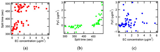
Figure 6.
Relationship between split time, PyC and EC concentrations: (a) Split time vs. EC concentration; (b) PyC vs. split time; (c) PyC vs. EC concentration.
As explained in Figure 6b, PyC was correlated with the split time. Figure 7a shows the relationship between PyC and the split time obtained in this study. A linear regression analysis for Post-Ox split time shows that the slope is 0.039 ± 0.007. Figure 7b is the PyC vs. split time adopted from another research group [25]. Linear regression analysis for Post-Ox split time from 673 s to 751 s shows that the slope is 0.007 ± 0.0007. It is noted that PyC is mainly positive for Post-Ox split time for both cases. It is difficult to directly compare our results to the other research group’s results because different protocols were employed. We used the NIOSH 5040 protocol, while the other group did the EUSARR2. In addition, the ranges of split time and the EC concentration were different from each other. It is certain that PyC is not zero any more at Post-Ox split time. Perhaps further study needs to better understand the rigorous relation between PyC and split time.
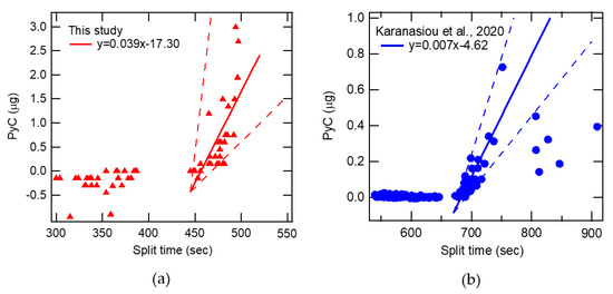
Figure 7.
PyC quantity as a function of split time: (a) This study; (b) Other study [25].
3.5. Limitations of this Study
This study shows PyC, EC concentration, split time and their relationships based on the analysis of samples collected for about 45 days, which is short to address seasonality on the relationships. The samples were collected at a university in the middle of Korea. Thus, the EC fractions obtained in this study reflect only a specific situation in Korea. Samples from various locations need to be analyzed in order to understand the spatial variation of PyC, EC, split time and their relationships, which is beyond the scope of this study.
4. Conclusions
A thermal-optical analysis was applied to deriving the correlation with respect to light-absorbing carbon based on EC and its fractions included in PM2.5 at KOREATECH, Byeongcheon Campus. The eBC was measured by the MAAP and samples were simultaneously collected with a sampler for OC/EC analysis. One of factors that made quantification of PyC difficult was the occurrence of Pre-Ox split time presumably caused by metal salts, mechanical failure of the analyzer, etc. Some EC fractions and their combinations were correlated with EC concentration. We examined the relationship between PyC and EC concentrations with respect to the split time. PyC was correlated with Post-Ox split times, while PyC was close to zero for Pre-Ox split times. We investigated the relationship between EC concentration and various EC fractions. EC3 and EC1 + EC3 turned out to be the dominant fractions for the quantification of EC in the present study. The hallmark of this study is that we examined the relationship between PyC and EC concentrations with respect to split time under NIOSH 5040 protocol for the first time as far as the authors know. PyC should be considered for the case of Post-Ox split times. Though this study was limited to a 45 days-long campaign, it was possible to observe the correlation between PyC and split time. Extensive sampling at various places and longer time is needed in order to identify temporal and spatial variations of PyC, EC and split time, which will be of interest for our future study. We believe that our study contributes to triggering active discussion about how to standardize the quantification of carbonaceous aerosols.
Author Contributions
Conceptualization, J.L. (Jeonghoon Lee); methodology, J.L. (Jeonghoon Lee); software, J.L. (Juhan Lee), D.K. and J.L. (Jeonghoon Lee); validation, J.L. (Jeonghoon Lee); formal analysis, J.L. (Juhan Lee), D.K. and J.L. (Jeonghoon Lee); investigation, J.L. (Juhan Lee) and J.L. (Jeonghoon Lee); resources, J.L. (Jeonghoon Lee); data curation, J.L. (Jeonghoon Lee); writing—original draft preparation, J.L. (Juhan Lee) and J.L. (Jeonghoon Lee); writing—review and editing, J.L. (Jeonghoon Lee); visualization, J.L. (Juhan Lee) and J.L. (Jeonghoon Lee); supervision, J.L. (Jeonghoon Lee); project administration, J.L. (Jeonghoon Lee); funding acquisition, J.L. (Jeonghoon Lee) All authors have read and agreed to the published version of the manuscript.
Funding
This work was supported by the National Research Foundation of Korea Grant funded by the Korean government (2019R1I1A3A01060938).
Institutional Review Board Statement
Not applicable.
Informed Consent Statement
Not applicable.
Conflicts of Interest
The authors declare no conflict of interest.
References
- Jacob, D.J.; Winner, D.A. Effect of climate change on air quality. Atmos. Environ. 2009, 43, 51–63. [Google Scholar] [CrossRef] [Green Version]
- Laden, F.; Schwartz, J.; Speizer, F.E.; Dockery, D. Reduction in Fine Particulate Air Pollution and Mortality. Am. J. Respir. Crit. Care Med. 2006, 173, 667–672. [Google Scholar] [CrossRef]
- Pope, C.A.; Muhlestein, J.B.; May, H.T.; Renlund, D.G.; Anderson, J.L.; Horne, B.D. Ischemic Heart Disease Events Triggered by Short-Term Exposure to Fine Particulate Air Pollution. Circulation 2006, 114, 2443–2448. [Google Scholar] [CrossRef] [PubMed] [Green Version]
- Lohmann, U.; Feichter, J. Global indirect aerosol effects: A review. Atmos. Chem. Phys. Discuss. 2005, 5, 715–737. [Google Scholar] [CrossRef] [Green Version]
- Slaughter, J.C.; Kim, E.; Sheppard, L.; Sullivan, J.H.; Larson, T.V.; Claiborn, C. Association between particulate matter and emergency room visits, hospital admissions and mortality in Spokane, Washington. J. Expo. Sci. Environ. Epidemiol. 2004, 15, 153–159. [Google Scholar] [CrossRef] [Green Version]
- Kaufman, Y.J.; Tanré, D.; Boucher, O. A satellite view of aerosols in the climate system. Nature 2002, 419, 215–223. [Google Scholar] [CrossRef] [PubMed]
- Park, S.S.; Bae, M.S.; Schauer, J.J.; Ryu, S.Y.; Kim, Y.J.; Cho, S.Y.; Kim, S.J. Evaluation of the TMO and TOT methods for OC and EC measurements and their characteristics in PM2.5 at an urban site of Korea during ACE-Asia. Atmos. Environ. 2005, 39, 5101–5112. [Google Scholar] [CrossRef]
- Schmid, H.; Laskus, L.; Jürgen Abraham, H.; Baltensperger, U.; Lavanchy, V.; Bizjak, M.; Burba, P.; Cachier, H.; Crow, D.; Chow, J.; et al. Results of the “carbon conference” international aerosol carbon round robin test stage I. Atmos. Environ. 2001, 35, 2111–2121. [Google Scholar] [CrossRef]
- Birch, M.E. Analysis of carbonaceous aerosols: Interlaboratory comparison. Analyst 1998, 123, 851–857. [Google Scholar] [CrossRef]
- Birch, M.E.; Cary, R.A. Elemental Carbon-Based Method for Monitoring Occupational Exposures to Particulate Diesel Exhaust. Aerosol Sci. Technol. 1996, 25, 221–241. [Google Scholar] [CrossRef]
- Chow, J.C.; Watson, J.G.; Pritchett, L.C.; Pierson, W.R.; Frazier, C.A.; Purcell, R.G. The dri thermal/optical reflectance carbon analysis system: Description, evaluation and applications in U.S. Air quality studies. Atmos. Environ. Part A Gen. Top. 1993, 27, 1185–1201. [Google Scholar] [CrossRef]
- Cavalli, F.; Viana, M.; Yttri, K.E.; Genberg, J.; Putaud, J.-P. Toward a standardised thermal-optical protocol for measuring atmospheric organic and elemental carbon: The EUSAAR protocol. Atmos. Meas. Tech. 2010, 3, 79–89. [Google Scholar] [CrossRef] [Green Version]
- Peterson, M.R.; Richards, M.H. Thermal-Optical-Transmittance Analysis for Organic, Elemental, Carbonate, Total Carbon, and OCX2 in PM2.5 by the EPA/NIOSH Method. In Symposium on Air Quality Measurement Methods and Technology-2002; Winegar, E.D., Tropp, R.J., Eds.; Air & Waste Management Association: Pittsburgh, PA, USA, 2002; Volume 83, pp. 1–19. [Google Scholar]
- Lee, J. Performance Test of MicroAeth® AE51 at Concentrations Lower than 2 μg/m3 in Indoor Laboratory. Appl. Sci. 2019, 9, 2766. [Google Scholar] [CrossRef] [Green Version]
- Cheng, Y.; He, K.-B.; Duan, F.-K.; Du, Z.-Y.; Zheng, M.; Ma, Y.-L. Ambient organic carbon to elemental carbon ratios: Influence of the thermal–optical temperature protocol and implications. Sci. Total Environ. 2014, 468–469, 1103–1111. [Google Scholar] [CrossRef] [PubMed]
- Cha, Y.; Lee, S.; Lee, J. Measurement of Black Carbon Concentration and Comparison with PM10 and PM2.5 Concentrations Monitored in Chungcheong Province, Korea. Aerosol Air Qual. Res. 2019, 19, 541–547. [Google Scholar] [CrossRef]
- Lee, J.; Yun, J.; Kim, K.J. Monitoring of black carbon concentration at an inland rural area including fixed sources in Korea. Chemosphere 2016, 143, 3–9. [Google Scholar] [CrossRef] [PubMed]
- Yang, H.; Yu, J.Z. Uncertainties in Charring Correction in the Analysis of Elemental and Organic Carbon in Atmospheric Particles by Thermal/Optical Methods. Environ. Sci. Technol. 2002, 36, 5199–5204. [Google Scholar] [CrossRef] [PubMed]
- Wang, Y.; Chung, A.; Paulson, S.E. The effect of metal salts on quantification of elemental and organic carbon in diesel exhaust particles using thermal-optical evolved gas analysis. Atmos. Chem. Phys. Discuss. 2010, 10, 11447–11457. [Google Scholar] [CrossRef] [Green Version]
- Birch, M. Elemental carbon (diesel particulate): Method 5040. In NIOSH Manual of Analytical Methods (NMAM); National Institute for Occupational Safety and Health: Washington, DC, USA, 1999. [Google Scholar]
- Xiaowei, L.; Jean-Charles, R.; Suyuan, Y. Effect of temperature on graphite oxidation behavior. Nucl. Eng. Des. 2004, 227, 273–280. [Google Scholar] [CrossRef]
- Oh, S.-H.; Park, D.-J.; Cho, J.-H.; Han, Y.-J.; Bae, M.-S. Intercomparison of Carbonaceous Analytical Results using NIOSH5040, IMPROVE_A, EUSAAR2 Protocols. J. Korean Soc. Atmos. Environ. 2018, 34, 447–456. [Google Scholar] [CrossRef]
- Reid, J.P.; Bertram, A.K.; Topping, D.; Laskin, A.; Martin, S.T.; Petters, M.D.; Pope, F.D.; Rovelli, G. The viscosity of atmospherically relevant organic particles. Nat. Commun. 2018, 9, 1–14. [Google Scholar] [CrossRef] [PubMed] [Green Version]
- Panteliadis, P.; Hafkenscheid, T.; Cary, B.; Diapouli, E.; Fischer, A.; Favez, O.; Quincey, P.; Viana, M.; Hitzenberger, R.; Vecchi, R.; et al. ECOC comparison exercise with identical thermal protocols after temperature offset correction–instrument diagnostics by in-depth evaluation of operational parameters. Atmos. Meas. Tech. 2015, 8, 779–792. [Google Scholar] [CrossRef] [Green Version]
- Karanasiou, A.; Panteliadis, P.; Perez, N.; Minguillón, M.; Pandolfi, M.; Titos, G.; Viana, M.; Moreno, T.; Querol, X.; Alastuey, A. Evaluation of the Semi-Continuous OCEC analyzer performance with the EUSAAR2 protocol. Sci. Total Environ. 2020, 747, 141266. [Google Scholar] [CrossRef] [PubMed]
Publisher’s Note: MDPI stays neutral with regard to jurisdictional claims in published maps and institutional affiliations. |
© 2021 by the authors. Licensee MDPI, Basel, Switzerland. This article is an open access article distributed under the terms and conditions of the Creative Commons Attribution (CC BY) license (https://creativecommons.org/licenses/by/4.0/).