Abstract
The Western Gulf of Corinth (WGoC) exhibits significant seismicity patterns, combining intense microseismic background activity with both seismic swarms and short-lived aftershock sequences. Herein, we present a catalogue of ~9000 events, derived by manual analysis and double-difference relocation, for the seismicity of the WGoC during 2013–2014. The high spatial resolution of the hypocentral distribution permitted the delineation of the activated structures and their relation to major mapped faults on the surface. The spatiotemporal analysis of seismicity revealed a 32-km-long earthquake migration pattern, related to pore-pressure diffusion, triggering moderate mainshock-aftershock sequences, as fluids propagated eastwards in the course of ~15 months. The anisotropic properties of the upper crust were examined through automatic shear-wave splitting (SWS) analysis, with over 2000 SWS measurements at local stations. An average fast shear-wave polarization direction of N98.8°E ± 2.8° was determined, consistent with the direction of the maximum horizontal regional stress. Temporal variations of normalized time-delays between fast and slow shear-waves imply alterations in the level of stress or microcrack fluid saturation during the long-lasting pore-pressure diffusion episode, particularly before major events. The present study provides novel insights regarding seismicity patterns, active fault structures, anisotropic properties of the upper crust and triggering mechanisms of seismicity in the WGoC.
1. Introduction
The Western Gulf of Corinth (WGoC), located in Central Greece, is one of the best-monitored seismogenic sites in Europe. Its high deformation rate (14–15 mm·yr−1 extension in a N9°E direction; [1,2]) is the driving force of the intense microseismic activity that has been recorded by the Corinth Rift Laboratory (CRL) local seismological network since 2000 [3]. The background microseismicity is interspersed by seismic swarms (e.g., [4,5,6,7]) and earthquake sequences [8,9,10]. The WGoC has been the site of major events, with the most recent one being the 15 June 1995 Ms = 6.2 Aigion earthquake [11]. The Gulf of Corinth is an active continental rift, formed by conjugate E-W-trending normal faults (Figure 1; [12,13]). Major structures of the southern flank of the WGoC include the north-dipping Aigion, Helike and Pirgaki faults, as well as the Psathopyrgos fault [14], linked with the Aigion fault via the en echelon Lambiri, Selianitika and Fasouleika NW-SE to WNW-ESE-trending fault segments (Kamarai fault system [11]). In the Greek Database of Seismogenic Sources [14], the Aigion fault is represented by a crustal-scale individual seismogenic source (GRIS503; Figure S20), whereas the Fasouleika and Selianitika faults are minor branches. Opposite to these structures, at the northern shore, the SW-NE-trending, SE-dipping Platanitis and Nafpaktos faults are mapped. Towards the east, the south-dipping Marathias and Kallithea faults are aligned E-W and WNW-ESE, respectively. Another south-dipping structure to the north of Marathias is the Trikorfo fault [14], extending eastwards to the Sergoula fault [15]. Offshore faults have also been mapped, such as the south-dipping Trizonia fault, the West Channel fault and the North and South Eratini faults [16,17].
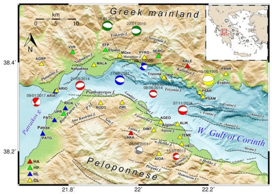
Figure 1.
Seismotectonic map of the Western Gulf of Corinth (WGoC; location marked by the red rectangle in the inset map). Beachballs depict the focal mechanisms of significant earthquakes: red after NKUA-SL, blue after GI-NOA, green for the 2010 Efpalio earthquakes after [29], yellow for the 1995 Ms = 6.2 Aigion earthquake [11] and gray for the 2001 Agios Ioannis Mw = 4.2 event [3,4]. Triangles depict seismological or accelerometric stations that operated during the study period (2013–2014), with colours corresponding to different network codes (legend at the bottom-left). Fault lines after [4,12,15,16,17,30]. Pt.f.: Panachaikon transfer-fault.
The background seismicity in the WGoC is scattered with epicenters, mainly located offshore between Aigion and Trizonia Island, but also north of the Psathopyrgos fault. Background seismicity rates are of the order of 10 events/day, automatically detected by the local CRL network, reaching hundreds of events/day during earthquake swarms or aftershocks [5,8]. This seismic activity, driven by high strain-rates, is associated with a fragmented seismogenic low-angle, north-dipping layer below the gulf, where the major normal faults of the region are rooting. Within the background seismic activity in the WGoC, long-term repeaters have been identified, associated with recurring slip on the same fault patch over the course of several years [9]. Such observations indicate the existence of small asperities surrounded by a partially creeping fault surface. Onshore seismicity is mostly projected towards the northern shores, near Efpalio and Eratini, mainly associated with activity at the deeper part of a north-dipping growing detachment (e.g., [8,9]).
Herein, we investigate the spatiotemporal evolution of the earthquake activity in the WGoC and examine patterns that could be associated with the involvement of aseismic factors driving the seismicity, such as propagating fluids or creeping of the surrounding fault surface. For this purpose, we also examine the anisotropic properties of the crust in terms of their statistics and temporal variations, which could be related with alterations in the level of stress or pore space fluid saturation. Seismic anisotropy in the upper crust is usually attributed to the presence of microcracks with a specific orientation [18]. As shear-waves propagate through an anisotropic medium, the Shear-Wave Splitting (SWS) phenomenon occurs, producing a fast shear-wave (Sfast) that becomes polarized to the direction favored by the medium’s anisotropic properties, whereas a slower one (Sslow) is polarized to a perpendicular direction. The Anisotropic Poro-Elasticity (APE) model considers the presence of vertical, fluid-saturated microcracks in the upper crust, taking into account the influence of the physical properties of the fluids [18]. The APE model attributes the SWS properties to the balance between the pore-fluid pressure and the local stress field, particularly its maximum horizontal component, σHmax [19,20]. It also ascribes variations of the SWS parameters to stress field changes, enabling their correlation with fluid processes, such as diffusion. Changes in the microcrack orientations or fluid saturation have been related to pore-pressure diffusion mechanisms associated with precursory stress-load on faults or post-seismic fluid release [21]. In Greece, a significant number of SWS studies have been performed. In the Eastern Gulf of Corinth [22,23,24], the Santorini Volcanic Complex [25] and Marathon [26], upper-crust anisotropy was attributed to the presence of stress-oriented fluid-filled microcracks, according to the APE model. However, there have also been observations where SWS has been related to CO2 degassing processes [27]. Since 1990, studies in the WGoC have revealed a relation between σHmax and the polarization direction of the fast S-waves (e.g., [11,28]). Since 2000, with the installation of the CRL network [3], the large amount of recorded microseismic events has rendered the region an ideal site for the study of variations of the SWS parameters.
In this work, we present a high-resolution earthquake catalogue of ~9000 events for the WGoC during 2013–2014, along with a large dataset of shear-wave splitting parameters. This period is characterized by several seismic swarms and mainshock-aftershock sequences, presenting complex dynamics. We apply double-difference relocation to reduce the relative location uncertainties between clustered events and to enhance the spatial resolution of the catalogue. We examine the spatiotemporal evolution of seismicity, focusing on earthquake migration patterns. We examine phenomena related to the diffusion of fluids or aseismic creep by means of earthquake migration speeds, hydraulic diffusivities and diffusion exponents, with respect to potential origin points of fluid injection. The above are studied in conjunction with the temporal variations of the SWS parameters, focusing on periods characterized by the occurrence of seismic swarms or major events producing aftershock sequences. We determined more than 2000 fast shear-wave polarization direction and time-delay measurements over a period of two years; a number significantly larger from what is included in most upper-crust SWS studies. The wealth of measurements ensures the validity and the reliability of the herein presented results. We examine the spatial distribution of relocated hypocenters through detailed cross-sections and provide a 3D interactive visualization to showcase the relation between the inferred activated structures at depth and the mapped faults on the surface. The present study aims to provide a high-resolution view of the active fault geometries in the WGoC and their interplay, as seismicity migrates from one structure to another. We further investigate and discuss the possible triggering mechanisms of seismicity associated with the observed migration patterns, providing further insights from the SWS analysis of the upper crust in the area of the WGoC.
2. Materials and Methods
The primary data used in this study are the recordings of the seismological stations of the CRL network and of the local stations of the Hellenic Unified Seismological Network (HUSN). These were acquired through the web services of the international Federation of Digital Seismograph Networks (FDSN); specifically, from the Réseau sismologique et géodésique français (RESIF; http://seismology.resif.fr/) (accessed on 9 July 2021), for stations of the CRL network, and from the National Observatory of Athens data center for the European Integrated Data Archive (EIDA@NOA; http://eida.gein.noa.gr/) (accessed on 9 July 2021), for stations of the HUSN [31]. In the following subsections, we present the various methodologies that were followed to process the available data and produce the results which are further described in Section 3.
2.1. Location and Relocation of the Catalogue
We employed a dataset of over 9000 events that occurred during 2013–2014 in the WGoC. Preliminary event detections and arrival-time data for these events were available from the websites of the Geodynamics Institute of the National Observatory of Athens (GI-NOA; https://bbnet.gein.noa.gr/HL/) (accessed on 9 July 2021) and CRL http://ephesite.ens.fr/~eworm/ (accessed on 9 July 2021). Additional P- and S-wave arrival time picks at local stations of CRL and HUSN were manually added to enrich the dataset, which herein is referred to as “Catalogue 1”, or briefly, Cat1.
Initial locations were obtained with the HypoInverse code [32], using the local velocity model of [33] for the WGoC. The only exception is the seismic cluster of the 2013 Helike swarm, for which an optimal velocity model [6] was employed. We applied a first approximation of station corrections, by removing the average P- or S-wave travel-time residual on each station and recalculating locations. At this point, we separated the dataset into spatial groups based on the hypocentral distribution. Initial locations indicated that seismicity related to the shallow structures of the WGoC reaches a depth of ~15 km. Seismicity at depths Z < 15 km was divided into clusters with the application of Ward’s [34] linkage to the matrix of inter-event hypocentral distances. Smaller clusters were merged by visual inspection to produce a total number of 9 spatial groups (Figure 2). The seismicity around the margins of the study area or deeper than 15 km was placed in a 10th “miscellaneous” group.
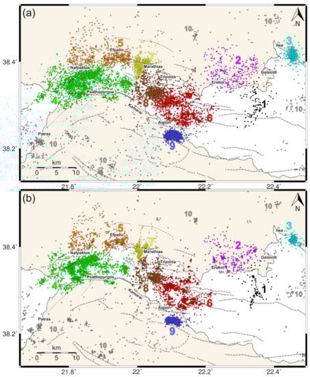
Figure 2.
Seismicity of years 2013–2014 in the Western Gulf of Corinth (a) before and (b) after relocation with HypoDD. Different colours and numbers represent the 9 spatial groups to which the dataset has been divided, in addition to the “miscellaneous” group (#10), presented in gray.
All the following procedures were performed independently for each spatial group. At least one reference station, in close proximity to the respective epicenters, was selected to perform waveform cross-correlation. Each recording was band-pass-filtered in the range 2–15 Hz (e.g., [6,25]) and then cropped in windows containing P, S and coda waves. A correlation matrix was constructed by registering the global maximum (XCmax) of the cross-correlation function between all event-pairs with available recordings at the reference stations. Then, a combined correlation matrix was calculated, taking into account the maximum value of the individual matrices for each event-pair. Nearest-neighbor linkage was performed and each group was divided into multiplets by selecting an optimal threshold, Cth. The latter is determined as the value that maximizes the difference between the size of the largest cluster and the sum of clustered events [35], with a minimum of 0.60. Finally, for event-pairs within each multiplet, cross-correlation was performed on the recordings of all stations with available phase-pick data, in windows containing only P- or S-waves, after alignment of the waveforms on their respective P or S arrival-times. The XCmax and its corresponding time-lag were registered on each case.
These data, along with catalogue travel-times, were used as input for the double-difference relocation code, HypoDD [36]. This algorithm performs iterative inversion to minimize the double-difference between observed and calculated travel-times in pairs of neighboring events. The HypoDD code relocates hypocenters by attributing their travel-time differences to their inter-event distance, reducing uncertainties caused by unmodelled velocity structure and arrival-time reading errors. As a result, spatially correlated events become more concentrated and aligned, increasing resolution and highlighting the activated structures. Location statistics for Catalogue 1 are presented in the Supplementary Section S1. In addition, magnitudes were calculated using a spectral fitting method, similar to the one applied by [6] for the 2013 Helike swarm. Details on this procedure are described in the Supplementary Section S2. Compared to the initial locations (Figure 2a), the map of relocated epicenters (Figure 2b) presents a clearer, enhanced image of the spatial distribution of the seismicity, with better defined sub-clusters within each of the 9 groups and fewer sparse events in the gaps among clusters. A robustness test for the relocation procedure is described in Section S1 of the Supplementary Material.
Besides Cat1, which contains a selection of manually revised events, the location of additional events was sought to provide more candidate events for SWS measurements. For this purpose, the automatic catalogue of CRL http://ephesite.ens.fr/~eworm/ (accessed on 9 July 2021) was employed, containing over 43,000 events that occurred during 2013–2014. After removing events that were already available in Cat1, a quick examination by visual inspection was performed. Events with low signal-to-noise ratio (SNR), or identified as regional/out-of-network events being erroneously located inside the gulf, were discarded. Afterwards, automatic picking was performed by applying auto-regression [35] and correlation detector methods (e.g., [37]), using the manually picked P- and S-waves as templates (see Section S3 in the Supplementary Material). In total, 10,493 events were automatically resolved and located with HypoInverse. As the solutions of these additional events are considered to be of lower quality, they were placed in a separate “Catalogue 2”, or Cat2. More details on Cat2 are presented in Supplementary Section S3 (Figure S7). The combination of the two datasets will be referred to as “Catalogue 3”, or Cat3.
2.2. Shear-Wave Splitting (SWS) Analysis
A preliminary set of 14,825 events from both the manual (Cat1) and the automatic (Cat2) catalogues were selected as candidate events for an upper-crust SWS analysis using local stations. The first selection criterion is the “shear-wave window” [38], which requires the S-wave seismic rays to arrive at an incidence angle smaller than 45°, to avoid the influence of converted pS phases. The Signal-to-Noise Ratio (SNR) is measured for a signal window containing the S-wave first pulses. This is performed for a pre-defined range of frequency bands used for the application of a band-pass Butterworth filter, and the filter yielding the highest SNR is selected [39]. Waveform recordings with SNR < 1.5 are discarded.
Seismic anisotropy at the upper crust is studied via SWS, which is quantified by two parameters: a) the polarization direction, φ, of the fast shear-wave and b) the time-delay, td, between the arrivals of the two split shear-waves at a receiver. To process this large dataset, we employed the open-source software Pytheas [40], which offers a variety of popular SWS analysis methods and has successfully been applied in recent crustal anisotropy studies (e.g., [26,41]). We adopt the Eigenvalue (EV) [42], rather than the Rotation-Correlation (RC) method [43], as the former is considered to be more reliable [44]. The EV method performs a grid-search at a pre-defined range of φ, td value pairs. For each grid point, the horizontal waveforms are rotated to all candidate Sfast and Sslow co-ordinates, according to the examined φ, and then Sslow is shifted by -td for all time-delay values in the pre-defined range. The covariance matrix of the corrected waveforms is calculated in a window containing the S-wave pulse, and the major and minor eigenvalues λ1 and λ2 are determined. The solution that yields the minimum λ2 is considered as the optimal pair of φ and td. A 95% confidence interval in the range of λ2 values around the optimal grid point is considered to define the measurement uncertainties δφ and δtd (Figure 3).
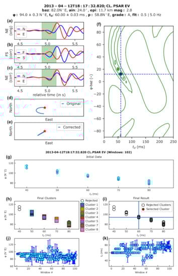
Figure 3.
Example of the automatic determination of the SWS parameters with the Pytheas software, using the Eigenvalue (EV) and Cluster Analysis (CA) methods. Horizontal recordings (a) in their initial N-S/E-W co-ordinate system (N-E), after the application of band-pass Butterworth filter between 0.5 and 5.0 Hz, (b) rotated into the Sfast/Sslow co-ordinate system (F-S), having measured φ = N94°E, then shifted Sslow leftwards by td = 60 ms and (c) rotated back to the N-S co-ordinate system, after being corrected for anisotropy, where the p = N58.8°E polarization direction is measured. The S-wave particle motion in the N-S co-ordinate system is also presented in the hodograms of panels (d) for the initial waveforms and (e) after correction for anisotropy. (f) Contours of the distribution of λ2 values during the grid-search of (φ, td) pairs performed for the application of the EV method, with the polarization direction displayed in the form of φ-baz, i.e., degrees relative to the back-azimuth, wrapped in a range of ±90° with respect to the R-axis direction. The selected (φ, td) pair, corresponding to the global minimum of λ2, is marked by the dashed cross-hair, pointing to the middle of a dark-shaded region that indicates the 95% confidence interval for λ2 [42], from which δφ = 0.3° and δtd = 0.03 ms are measured. (g–k) Diagrams of the Cluster Analysis (CA) method for the determination of the best window presenting: (g) the (φ, td) measurement pairs, (h) the performed clustering, (i) the selection of the most constrained cluster and measurement with the smallest errors, (j) the series of φ and (k) the series of td measurements per trial window index, with their respective uncertainties.
An important advantage of the Pytheas software is that it permits fully automatic SWS processing by defining the optimum S-wave signal window. This is performed with the application of a Cluster Analysis procedure [45]. A series of different window configurations are examined, within the bounds of the middle of S-P interval and the dominant period of the S-wave pulse multiplied by a user-defined factor [39,40]. For each window, φ and td are measured using the EV method and the solution pairs are sorted into clusters [45]. Then, the window yielding the (φ, td) solution pair with the smallest errors from the most constrained cluster is selected. The quality of the SWS parameter measurements is assessed by automatically calculating a score value, taking into account the ratio between δφ or δtd and a respective user-defined maximum threshold. A quality grade between A (best) and E (worst) is then attributed, depending on their resulting average score. The E grade is also reserved for cases of low SNR < 1.5. In the following, only measurements with grades A, B or C were taken into consideration. Furthermore, measurements are marked as “null” when their φ value is within ±10° from p or p + 90°, i.e., sub-parallel or perpendicular to the polarization direction, p, of the corrected (for anisotropy) shear-wave. In those cases, it is not possible to distinguish whether the medium is isotropic or the initial polarization coincides with that of the Sfast or the Sslow, which is why “null” measurements are discarded [46].
Figure 3 shows an example of the automatic analysis with the combination of the EV and CA methods for an event recorded at station PSAR. Initially, the automatic filtering algorithm decided the optimal band-pass Butterworth filter range between 0.5 and 5.0 Hz. Then, SWS measurements were performed in 102 trial signal windows. For each window, the EV method was applied to determine the φ and td values. The horizontal components were first rotated into the Radial-Transverse (R-T). Then, grid-search was performed, rotating the waveforms to the various φ values between R−90°T and R90°T, and shifting the transverse component leftwards by a time-delay td between 0.0 and 250.0 ms. In this example, the solution pair that yielded the minimum λ2 value was φ = Ν94.0° Ε ± 0.3° and td = (60.00 ± 0.03) ms in a 95% c.i. with grade “A”, indicating a measurement of the best quality. Figure 3g presents the selection of the optimal solution. It is noteworthy that despite the φ values being spread in a range roughly between 80° and 120°, the majority are clustered near the selected value of 94°, with the respective td at 60 ms (the preferred value). The diagram of Figure 3f shows the global minimum of λ2 for the selected signal window, marked by the dashed cross-hair. The validity of the φ, td measurements is verified in Figure 3e, where the resulting particle motion becomes nearly linear after the removal of anisotropy.
We verified the instrument orientation during the study period (2013–2014) using the method of [47], to ensure the validity of the polarization direction measurements. This method compares the polarization direction of teleseismic P-waves with the respective back-azimuth of the epicenters to determine the orientation of the positive direction of the instrument’s N-S component, which should be pointing towards the North. The results were compared with the orientations documented in the metadata of the stations supplied by the FDSN web services. Significant differences were identified at stations MG06 (N-S azimuth = N83°E) and the temporary station HELI (N-S azimuth = N340°E). The method of [47] was not applied to station ALIK, as it could not properly record the teleseismic waveforms. In that case, an orientation correction of N299°E was adopted after [48], who followed a similar approach, but using the P-wave polarization determined by local earthquakes [35]. For other stations, especially for borehole instruments, the nominal orientations supplied in the stations’ metadata were verified.
Out of the 14,825 candidate events from both catalogues, a total of 37,263 initial SWS results (15,083 from Cat1 and 22,180 from Cat2) were acquired, with 10,456 events providing a result from at least one station. Other events were discarded due to low SNR or errors during processing, in particular at the clustering stage. In the combined Cat3, 25,266 measurements with grade Ε and 4223 with grade D were rejected due to low quality. In addition, 3298 measurements were considered as null, having φ values sub-parallel or sub-perpendicular to the corrected source polarization, p. Finally, in Cat3, 192 valid measurements are with grade A, 1299 with grade B and 2985 with grade C, summing up to 4476 (Table S3 in the Supplementary Material).
3. Results
3.1. Spatial Distribution of Seismicity
A total of 8944 events of Cat1 were successfully relocated. As presented in the cross-sections of Figure 4, seismicity is mainly concentrated on a low-angle seismogenic layer at depths between 6.5 km and 10 km below the gulf (see also Figure S1d), reaching ~12 km down-dip the activated structures. Several clusters, mainly related to the occurrence of larger events, indicate the activation of higher-angle faults, rooting at the weak layer. The latter is further supported by the reported focal mechanisms (Table 1). The magnitudes of major events mentioned in the present study refer to their respective Mw values calculated herein by spectral fitting (see Section S2 in the Supplementary Material).
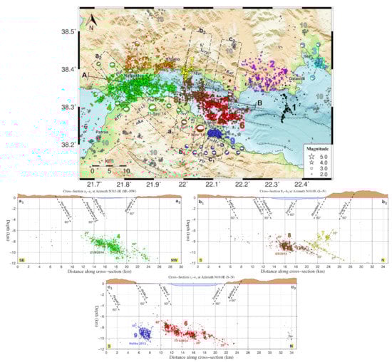
Figure 4.
(Top) Map of the relocated seismicity for the period 2013–2014 in the WGoC. Colours and numbers correspond to the 9 spatial groups into which the dataset was divided, as well as the “miscellaneous” group #10 (gray). Beachballs depict the focal mechanisms of major events (Table 1). (Bottom) Vertical cross-sections a1–a2 to c1–c2, corresponding to the dashed rectangles shown on the map (top). Beachballs depict the far hemisphere projections of focal mechanisms for the major events. Black dashed lines at the top of the cross-sections indicate the position of mapped active faults, with a typical down-dip extension at 60°, while coloured dashed lines indicate the inferred dip of activated structures at depth, according to the hypocentral distribution and/or focal mechanisms. Fault name abbreviations on the map, aKa: Ano Kastritsi f., Pt.f.: Panachaikon transfer-fault, RPfz: Rion-Patras fault zone, Psa: Psathopyrgos f., Plat: Platanitis f., Mar: Marathias f., Serg: Sergoula f., Kal: Kallithea f., Triz: Trizonia f., Sel: Selianitika f., Fas: Fasouleika f., wHe: West Helike f., Pir: Pirgaki f.

Table 1.
Focal mechanisms of significant events during 2013–2014 in the WGoC. Sources: NKUA 1 (Seismological Laboratory of the National and Kapodistrian University of Athens), NOA 2 (Geodynamics Institute—National Observatory of Athens) and K2015 [6]. Latitude, longitude, (centroid) depth and moment magnitude Mw* values are those reported from the respective reference. Mw is the moment magnitude determined by spectral fitting in this study and CLID is the spatial group ID (see Figure 4). Three important events of the dataset, related to specific sequences, are marked with bold.
The westernmost part of the Nafpaktos-Psathopyrgos group #4 (green), activated after the 21 September 2014 Mw = 4.6 event, could possibly be associated with the Rion-Patras SW-NE-trending dextral oblique-normal fault zone, or with related sub-parallel structures dipping towards NW. The N10°E cross-sections of Figure S13 imply gradual deepening of seismicity towards the western profiles, which is also highlighted in Figure 4a1–a2, as well as in the N315°E-oriented cross-sections of Figure S14 and the N100°E-oriented cross-section of Figure S15. However, the focal mechanisms associated with the larger offshore events of group #4 (e.g., the 21 September 2014 Mw = 4.6 earthquake) suggest an E-W to WSW-ENE-striking fault. The latter, along with the hypocentral distribution, could indicate an association with the Ano Kastritsi fault, further south. The two available focal mechanisms for events below Platanitis support SW-NE faulting, with one being normal and the other dextral, both compatible with the kinematics of the Rion-Patras fault zone.
The N10°E cross-section b1–b2 of Figure 4 contains seismicity of groups #7 (yellow) and #8 (brown), the latter associated with the June 2014 outburst in the gulf. Although the seismic activity is mostly compacted in the depth range 8–10 km, distinct clusters can be associated with individual structures, some being located at shallower depths (6–8 km) towards the north. The 8 June 2014 Mw = 4.3 event was likely hosted on a north-dipping structure, with a ~45° dip according to the focal mechanism reported by NKUA (Table 1). This makes it partly compatible with the Fasouleika fault segment, if a small degree of listricity is considered. Likewise, the different strike (NW-SE) of the 24/01/2014 Mw = 3.9 event could support an association with the Selianitika or Lambiri faults. Seismicity at the northern part of the group #8 is distributed on a gently dipping layer, with a dip of ~23°. This is sub-parallel to the seismicity of group #7, further north, which seems to spread deeper and northwards along the same trend (Figure 4b1–b2, dashed yellow line with a northwards dip of ~27°). Shallower seismic activity in group #7 could be related with antithetic, south-dipping structures, such as the Sergoula fault which is associated with the eastern part of the Trikorfo seismogenic source (GRCS441 in [14]; Figure S20).
Another important profile is presented in the cross-section c1–c2 of Figure 4, which includes groups #6 and #9. The 2013 Helike swarm (group #9, blue) occurred mainly in the depth range of 8–10 km. A detailed analysis of this swarm [6] has revealed focal mechanisms associated with both north-dipping normal faulting and oblique-normal faulting. Such kinematics have also been observed for the 2001 Agios Ioannis swarm [4,8,49], associated with the northwest-dipping Kerinitis fault. The extension of the north-dipping fault plane of the 2013 Helike swarm to the surface is traced near the junction between Pirgaki and Kerinitis faults [6]. The relation of these faults to the structures activated during the 2013 Helike swarm is presented in Figure S25 (see also the provided interactive Matlab figure; File S1). It should be noted that the Pirgaki fault is likely a branch of the Mamousia seismogenic source (GRCS524 in [14]; Figure S20).
The southern seismicity in group #6 (red) is mostly part of the aftershock sequence of the 7 November 2014 Mw = 4.8 event and appears to be associated with the west Helike fault. The focal mechanism of the mainshock suggests a northwards dip of 30°, while the hypocentral distribution of its aftershocks (south of its epicenter) corresponds to a roughly ~40° dip. The latter could indicate some degree of listricity, or the existence of multiple smaller activated structures within the seismogenic layer, each dipping at a higher angle (e.g., 60°). Seismicity of group #6 extends further north, with the focal mechanism of a smaller event that occurred on 28 January 2013 having a dip of 28°. This low dip angle is similar to that of the northern part of group #8 (brown), as well as of the deeper part of group #7 (yellow). It is noteworthy, however, that when examined in a N100°E cross-section (Figure S15, along the Kamarai fault zone), there appears to be a vertical offset between these shallow dipping segments of groups #4, #8 and #6, tending to deepen from west to east (see also File S1). This is likely related to the en echelon faulting configuration at the southern shoulder of the WGoC.
Other parts of seismicity (Figure S13) include the northern groups #5 (orange, between Nafpaktos and Pyrgos, i.e., station PYRG) and #2 (magenta, near Eratini; Figure 1). Both are associated with sparse seismicity on a shallow-angle, north-dipping plane, reaching depths larger than 10 km below the northern coast. Group #1 (black), likely related with the deeper and almost flat sector of the South Corinth Gulf composite seismogenic source (GRCS500 in [14]; Figure S20), follows the trend of group #2 southwards at depths of 8–12 km. At the eastern margin of the study area, the isolated cluster #3 (cyan) is associated with a nearly dip-slip faulting type (Figure 4, Table 1) on a sub-vertical WNW-ESE-trending fault, slightly tilted northwards. Seismicity in the miscellaneous group #10 (gray) includes activity around the margins of the study area or deeper than 15 km. The latter is the case for events southwest of group #4, in the form of small clusters located at depths of ~17–22 km. Some deeper events are also located below Aigion, including an Mw = 4.0 earthquake that occurred on 28 April 2013 at a depth of 47 km with its epicenter offshore, east of group #9.
3.2. Spatio-Temporal Analysis of Seismicity
The temporal evolution of seismicity in the WGoC during 2013–2014 is examined in terms of seismicity rates, spatiotemporal seismicity migration speeds and pore-pressure diffusion. Figure 5 (top) shows the cumulative number of events per spatial group, for selected seismicity above the magnitude of completeness, which is estimated at Mc = 1.8 for the manual dataset (Figure S19). The application of this threshold enhances the occurrence of seismicity bursts, usually triggered by events of larger magnitude, related to specific sequences whose initiation is marked by vertical gray lines in Figure 5. Some spatial groups are characterized by generally constant background seismicity rates, i.e., ~0.1 events/day in group #1, 0.2 events/day in group #2 and 0.4–0.5 events/day in group #5. The miscellaneous group #10 (gray) presents a background seismicity rate of 0.4–0.7 events/day, increased to ~1.1 events/day in the second half of 2014. In other groups, their low seismicity rates, excluding periods of bursts, range between ≤0.1 and 0.6 events/day. A general sense of the spatial distribution of background seismicity in the WGoC can be observed during January–August 2013 (Figure S22a). During that period, the more significant cluster was the 2013 Helike swarm in the south, whereas only sparse seismicity and small clusters are distributed in the rest of the study area.
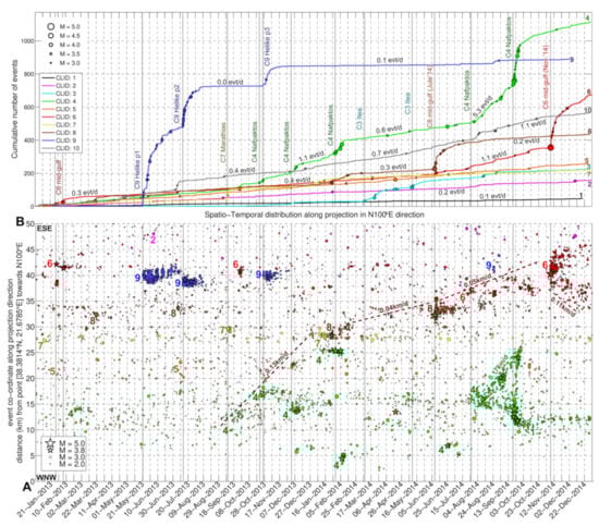
Figure 5.
(Top) Cumulative number of events per spatial group (colours/numbers) for events with Mw ≥ Mc = 1.8 of the manual, relocated catalogue of the 2013–2014 seismicity at the WGoC (Cat1). Seismicity rates are marked in events per day (evt/d). The occurrence of events with Mw ≥ 3.0 is marked by circles on each curve. (Bottom) Spatiotemporal projection of epicenters (without magnitude threshold) along the N100°E-oriented profile line A–B of Figure 4 (top). Spatial groups associated with the occurring seismicity are marked by numbers and represented by their respective colours. Inferred seismicity migration patterns are marked by dashed lines, with migration speed in km/day. The initiation of significant sequences is marked by gray vertical lines and labels at the top panel (C# refers to the spatial group number #).
Figure 5 (bottom) shows the projection of epicenters along the N100°E profile line A–B (Figure 4, top) with respect to the origin time, without filtering out events with Mw < Mc. In early 2013, most seismic activity was concentrated mid-gulf at group #6 (red), following an Mw = 3.8 event on 28 January 2013, and at group #8 (brown) with a few minor bursts. Groups #2 (magenta), #4 (green), #5 (orange) and #7 (yellow) exhibited relatively constant seismicity rates of 0.2–0.4 events/day. Then, on 21 May 2013, the first phase of the Helike swarm (group #9, blue) was initiated with a series of events reaching Mw 3.6–3.7, mainly activating the eastern half of the cluster. The activity in Helike culminated with a second phase during July, involving an Mw = 3.8 event on 15 July 2013, which triggered seismicity at the western part of the group. The first two phases of the swarm, until August 2013, are described in detail by [6]. A third phase began on 26 October 2013, lasted for about 20 days and was concentrated at the mid-northern part of the cluster. Group #7, near Marathias, presented a small burst of activity in early September 2013.
An increase in the seismicity rate to ~1.1 events/day began in October 2013 at the offshore group #4, in the region between Nafpaktos and Psathopyrgos, presenting bursts associated with the occurrence of larger events (Mw ≥ 3.0). This first wave of seismic activity in group #4 lasted up to February 2014, with its seismicity rate returning to 0.6 events/day. Seismicity of group #4 was initially concentrated in the Y-range of 10–20 km (Figure 5, bottom), but gradually spread bilaterally towards Y = 25 km in January and Y = 5 km in February 2014. At that time, the seismic activity was also increased, temporarily, in the neighboring groups #7 (yellow) and #8 (brown). The isolated cluster #3 (cyan) near Itea presented swarm-like activity between 8 March and 14 September 2014, following a series of events, the largest being an Mw = 4.0 on 10 May 2014.
On 8 June 2014, 15:10:51 UTC, an Mw = 4.3 event initiated an aftershock sequence in group #8, at the offshore region SW of the Trizonia Island, lasting for about one month. Increase in the seismicity rate of group #6 (red), including several Mw ≥ 3.0 events, began in July 2014 (Figure A1). Part of that group was triggered by the 8 June 2014 event in group #8 (Figure A2), likely due to the partial overlap between the involved structures, as these groups cannot be fully distinguished with spatial margins. More importantly, a significant pattern of bilateral seismicity migration began to emerge in mid-July 2014 in group #4, originating at Y ≈ 15 km (Figure 5, bottom), spreading towards Y = 25 km and Y = 10 km in a period of two months. Seismic activity at the western part of group #4 was abruptly increased in the form of an aftershock sequence after the occurrence of an Mw = 4.6 event on 21 September 2014 [48]. The last major seismicity outbreak at the WGoC during the study period began on 7 November 2014, with an Mw = 4.8 event in group #6 (red), offshore Aigion [48]. The seismic activity spread rapidly in the form of an aftershock sequence, bilaterally along a ~7-km-long patch in an E-W direction (Figure A3), but mostly south of the mainshock’s epicenter (Figure S22c).
Regarding the physical mechanisms behind the spatiotemporal seismicity migration patterns, stress-transfer and pore-pressure diffusion are considered. Slip occurs when the applied shear stress on a fault plane, aided by the pore-pressure in fluid-filled microcracks, surpasses the sum of the cohesive strength of the material and the internal friction. Changes in the level of stress in a specific location may result from Coulomb stress transfer due to the occurrence of an earthquake in a nearby region, which is the main mechanism behind the triggering of aftershocks. Aseismic slip, e.g., due to creeping, also causes Coulomb stress changes that may load a neighboring area, accelerating earthquake occurrence, or relaxing another region. Finally, the diffusion of pressurized fluids can generate earthquakes in the volume behind a triggering front that spreads through the fracture network, increasing pore-pressure and lowering the effective normal stress on a fault plane, thus facilitating slip.
When fluids are injected in a homogeneous and isotropic, poro-elastic, fluid-saturated medium, the expanding spherical triggering front of induced seismicity follows Equation (1) [50]:
where r(t) is the triggering front’s radius (distance from the injection point), t is the time since the beginning of the pore-pressure perturbation at time to and D is the hydraulic diffusivity. The same principle may apply as a first approximation to a fluid-saturated crust and an initial pore-pressure perturbation.
The determined spatiotemporal seismicity migration rates (Figure 5, bottom) provide a first indication regarding the possible physical triggering mechanism of seismicity in the WGoC. Initiating in September 2013, offshore Nafpaktos, seismicity started to migrate eastwards at a speed of ~0.13 km/d and then slowed down to 0.04–0.05 km/d after February 2014. Figure 6 shows the spatiotemporal evolution of the offshore groups #4, #8 and #6 (from west to east), mostly confined below the bold parabolic envelope drawn after Equation (1) with D = 2.2 m2/s. This triggering front starts in September 2013 at the Y ≈ 12 km position along the A-B profile line of Figure 4 (top). As the fluids propagate eastwards, earthquake sequences are triggered in bursts near the expanding front. This suggests a combination between pore-fluid pressure diffusion through the fracture network and seismic swarms occurring along the way. The latter evolve with additional stress transfer due to tectonic slip. In natural fluid injections, the time, location and geometry of the injection source can only be deduced by the observed seismicity migration patterns. In that sense, secondary triggering front envelopes can be inferred for each sub-sequence, e.g., at Y ≈ 15 km in mid-December 2013 or near Y ≈ 25 km in January-February 2014, with D = 0.5 m2/s.
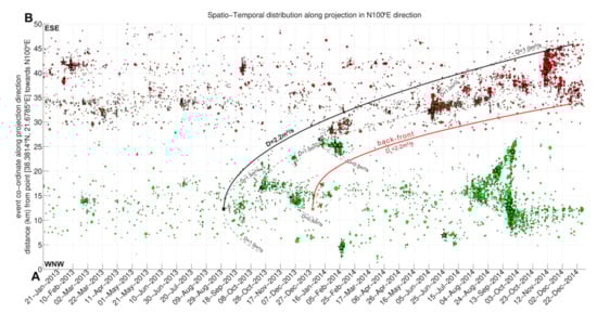
Figure 6.
Same as Figure 5 (bottom), but with seismicity of groups #4, #8 and #6 from Cat3, without magnitude threshold. Relevant seismicity migration patterns are marked by dashed black parabolic envelopes following Equation (1). A proposed back-front envelope is drawn with a red line after Equation (2), corresponding to the triggering front envelope with D = 2.2 m2/s, marked with a bold black line.
An eastwards-propagating patch with a width of ~10 km seems to be active behind the D = 2.2 m2/s triggering front. However, a deficit of seismicity is observed west of that patch (Figure 6). The latter indicates that the initial fluid injection was likely terminated and a back-front rb(t) is formed according to the relation [51]:
where td is the duration of the injection and Db the hydraulic diffusivity corresponding to the back-front. In Figure 6, a back-front curve of Db = 2.2 m2/s is shown with a bold red line, beginning ~120days after the initiation of the triggering front at point Y ≈ 12 km on 1 September 2013. In that case, the post-injection hydraulic diffusivity is the same, considering pore-pressure diffusion in three dimensions (Equation (2); [51]).
Meanwhile, in July 2014 the Nafpaktos-Psathopyrgos swarm began to evolve, starting very close to the supposed injection site at Y ≈ 15 km (dashed red ellipse in Figure S22b,c). However, its evolution cannot be fit with a parabolic envelope, but is better approximated by a roughly linear triggering front, up to a point when it even tends to accelerate as it spreads (Figure A4). Its seismicity migration speed was 0.13 km/d eastwards and 0.03–0.07 km/d westwards between 15 July and ~20 August 2014 and then the eastwards migration speed increased to 0.17 km/d. The 21 September 2014 event caused seismicity to spread eastwards at over 0.35 km/d, while the western branch began to expand rapidly at over 1 km/d. The latter speed is likely too fast to be associated with pressurized fluids in a tectonic environment and is more akin to triggering by aseismic slip (e.g., [52]).
We also estimated the mean squared distance (msd) of seismicity with time t, which provides a proxy for the rate of triggered earthquake migration [53]. In normal (Gaussian) diffusion, the msd scales linearly with t. Instead, the hallmark of anomalous diffusion is the non-linear scaling of the msd with t, that frequently takes the form of a power-law (e.g., [54]):
The power-law, or diffusion exponent a, characterizes the various domains of the diffusive process, designating sub-diffusion for 0 < a < 1 and super-diffusion for a > 1, while for a = 1 normal diffusion is recovered.
Taking as an approximate reference (x0 = 0, t0 = 0) the Y ≈ 12.3 km position along the A-B profile line of Figure 4 (top) on 1 September 2013 (similar to the reference point of the triggering front shown in Figure 6), we estimate the msd of seismicity with time. This is performed for the events with Mw ≥ Mc, enclosed within the parabolic envelope defined by the triggering- and back-fronts of seismicity for D = 2.2 m2/s (Figure 6). The msd is calculated as ([49]):
where xn(t) is the distance of the nth event from the reference point at time t and N is the total number of events. The result is shown in Figure 7 in double-logarithmic axes and logarithmically spaced bins. The overall growth of the msd with t signifies the diffusive process. This growth is not continuous, but rather evolves in sequential “steps”, as observed after the passage of ~50, 130, 272 and 418 days (Figure 7). These days mark the activation of the sequential seismic clusters in groups #4, #6 and #8 towards the east, within the parabolic envelope defined in Figure 6. On the other hand, during the in-between time periods, the msd is almost constant or grows slowly with t. The overall scaling behavior of the msd with t can be approximated with Equation (3), yielding a diffusion exponent a = 1.81 ± 0.17 (R2 = 0.98). In terms of the Continuous Time Random Walk (CTRW) model (e.g., [55]), this value of the power-law exponent indicates super-diffusion. Compared to the range of exponents reported in the literature that mainly correspond to slow earthquake sub-diffusion [49,56,57,58,59,60], the diffusion exponent in this case is significantly larger and comparable to that reported by [61]. Hence, the large diffusion exponent likely corresponds to large rates of earthquake migration triggered by aseismic factors, such as pore-pressure diffusion or aseismic creep.
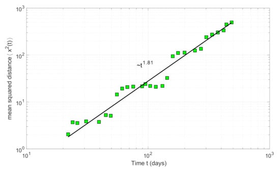
Figure 7.
Mean squared distance ⟨x2(t)⟩ of seismicity (squares) with time t in double-logarithmic axes, for the events enclosed within the parabolic envelope defined by the triggering- and back-fronts of seismicity with D = 2.2 m2/s (Figure 6). The solid line indicates the power-law growth of ⟨x2(t)⟩, according to Equation (3).
3.3. Shear-Wave Splitting Parameters
The distribution of the fast shear-wave polarization direction (φ) measurements from Cat1 for selected stations, representing sites with different average φ directions, is presented in Figure 8 in the form of rose diagrams. The respective diagrams for the rest of the stations are available in Figure S16. Rose diagrams, widely used in shear-wave splitting studies (e.g., [22]), are circular histogram plots which display directional data (in the current case, fast shear-wave polarization direction data) and the frequency of each class, (i.e., the number of measurements for each φ bin). The SWS parameter statistics for Cat1 are presented in Table 2. The average φ value is calculated with circular statistics [62] to avoid wrapping between 0° and 180°. In most stations, the mean value coincides with the direction that corresponds to the larger amount of valid measurements. There are, however, a few exceptions, such as station HELI (Figure S16), which presents two main fast-shear-wave polarization directions, one at ~N30°E and another at ~N100°E. The mean φ in that case was calculated at 77.6° ± 11.6°. However, this value does not correspond to either of the two maxima of the distribution. There are also some stations with significant φ scatter, such as VVK, and certain stations of the Magoula array, i.e., MG03, MG05 and MG07, for which the mean value differs from the azimuth that corresponds to the maximum of measurements. The value of valid measurements for all stations (Cat1) is 98.8° ± 2.8°. Important deviations from this direction are observed for stations LAKA ( = 134.7° ± 5.9°) and TEME ( = 145.1°±16.3°), in the south, and stations SERG ( = 58.4°±7.5°) and MALA ( = 68.1° ± 11.0°), in the north. Stations with significant φ scattering, indicated by the large uncertainty, include MG03 ( = 67.1° ± 30.8°), PANR ( = 132.8° ± 36.6°) and PYRG ( = 142.2° ± 41.6°). The time-delays, td, are partially depended on the spatial distribution of the seismic sources relative to the receiver. Since the time-delay is accumulated along the path-length of the seismic ray as it travels through the anisotropic medium, longer ray-paths will result in larger td values. The time-delays are normalized (tn) by dividing td with the hypocentral distance to remove the effect of the ray-path length. The mean tn values are overall (9.2 ± 0.1) ms/km, while average tn per station ranges from 5.0 ms/km (AGRP) to 12.5 ms/km (ALIK). The raw td measurements have a mean of (112.3 ± 1.4) ms.
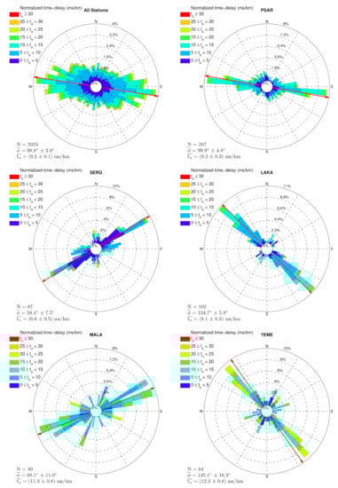
Figure 8.
Rose diagrams of the distribution of the fast shear-wave polarization angle, φ, for valid measurements with grade A (best) to C (acceptable) from Cat1 (only manually located/relocated events) per station (station-code shown in the label on top of each diagram), for selected stations representing sites with different average φ directions, as well as for all stations (upper-left panel). Colours correspond to the respective normalized time-delay, tn. The total number of measurements (N) and average φ and tn are presented at the bottom-left of each panel. The red arrows indicate the average φ direction. See Figure S16 for rose diagrams of the other stations.
Table 2.
Mean values of SWS parameters, i.e., mean polarization direction of the fast shear-wave,, mean time-delay between the two split shear-waves, , and mean normalized time-delay, , along with their respective uncertainties per station for valid measurements (grade A-C) of Cat1. Errors correspond to the 95% c.i. of the mean value, whereas and are the respective typical errors of the mean. N is the number of valid measurements per station. The first line in bold corresponds to all valid measurements of Cat1. The last column, “OC”, indicates the orientation correction applied on some stations, given in the form of the true azimuth of the instrument’s N-S component.
The distribution of φ values for null measurements, with φ being within ±10° from p or p + 90°, i.e., sub-parallel or perpendicular to the polarization direction of the corrected (for anisotropy) shear-wave, p, is presented in Figure S17. The distribution for all stations indicates a null = 5.4° ± 6.1°, i.e., in an approximate N-S direction, that is perpendicular to the respective of the valid measurements. This suggests that the majority of null φ values likely correspond to the polarization direction of the Sslow wave. However, there are (fewer) cases where φnull measurements of certain stations are similar with their , e.g., SERG (null = 64.9° ± 12.1°). In most stations, the average tn for null measurements is larger than the respective for valid ones.
Regarding the temporal variations of the SWS parameters, we take advantage of the large number of measurements from the combination of the manual and automatic catalogues to investigate patterns of change with time. The time-delay between the Sfast and Sslow waves, normalized by the ray-path length, can be used as an indicator for the degree of anisotropy in the medium. However, factors besides the traveled distance also affect td. These include the difficulties in the precise measurement of φ or td related to the radiation pattern (focal mechanism), the distortion of polarization due to non-perpendicularity of the incident seismic rays to the surface, variations in the frequency content between Sfast and Sslow and larger attenuation of the Sslow [44,63], effectively contributing to a significant degree of scatter. To exclude measurements that are less affected by changes in the geometry of the fluid-filled microcracks, we select event-station pairs whose ray-paths belong to “Band-1”. This is defined as the double-leafed solid angle between 15° and 45° on either side of the vertical crack-plane (whose azimuth is defined by ) passing through the station (see Figure S21 for a schematic view of Band-1). Ray-paths of event-station pairs travelling through the ±15° solid angle from the crack-plane are classified as “Band-2” measurements and are more affected by the microcrack density [64]. Optional filters are applied to remove part of the tn measurements, such as those affected by a higher angle of incidence at the surface, having strong spatial dependence or having a lower quality grade. In addition, temporal variations of tn are also examined after discarding results related to φ measurements that significantly differ from the of that station measured from Cat1, which may be potentially erroneous. For events of Cat2 (automatic), we applied a focal depth correction, as their lower quality hypocenters tended to be scattered at much shallower depths than their neighboring events of Cat1, causing inconsistencies in the tn dataset of Cat3. This was performed by applying, for each event of Cat2, the average focal depth of the events of Cat1 with neighboring epicenters (excluding those with Z > 15 km). This modification reduces some outliers in Cat2 that yielded erroneously high tn values due to the shorter distance (shallower depth). Small fluctuations of ±1 km or even ±2 km from that average depth don’t seem to affect the measured tn significantly, as the resulting changes are much smaller than the observed measurement scatter.
We focus on patterns of significant linear increase or decrease of tn values observed at more than one station during specific periods, as this may suggest a change that could be related to more widespread stress variations. To assess this task, we performed a series of linear regressions on sliding windows along the tn data (with or without the application of the above-mentioned filters) versus origin time. The regressions were applied using a range of different window-lengths, measured either in number of successive data points or days, to allow for various time scales and data densities to be taken into account. For each window, least-squares inversion is performed to calculate the best-fit line, along with the respective correlation coefficient, R2. On each case, the Student’s t-test is performed to examine whether the null hypothesis of zero slope can be rejected with a 95% confidence interval, and cases with p > 0.05 are discarded. We then examined the results and identified patterns of increase or decrease, which either persist or emerge, as stricter filters are applied. Furthermore, we examined periods during which a group of stations presented the same behavior regarding the tn change, whereas another group exhibited the opposite change behavior. The 3-point moving average is also calculated, to account for non-linear temporal variations or weak correlations.
Figure 9 shows the tn temporal variations for selected stations. In all cases, Band-1 was selected, while filtering out measurements with φ outside the ± 30° range (with as determined from Cat1) usually manages to further reduce scattering. Certain common characteristics are identified between different stations. In January-April 2013, stations PSAR, KALE and ZIRI exhibit a moderate decrease of tn values. Weak decrease is also observed at stations TRIZ and PYRG, whereas station SERG has increasing tn values during February-May 2013. That is the period before the occurrence of the 2013 Helike swarm. Station TRIZ presents a mild increase of tn in the period of May-July 2013, while time-delays at PYRG and ALIK (with events from groups #6 and #8 only; Figure 9) also follow a weakly increasing trend that lasts until December 2014. On the other hand, in October 2013–January 2014, several stations in the north present a significant decrease of tn values, including PSAR, KALE, TRIZ and most of the stations of the Magoula array, e.g., MG04 (Figure 9). One of the trend lines of station PYRG also indicates a strong decrease of tn between November 2013 and March 2014. This period could be of particular significance, as it coincides with the time when the proposed seismicity triggering front of Figure 6 passes near the middle of profile A-B (Y ≈ 25 km). On the contrary, some stations in the south, such as AIOA and ALIK (the latter for events of groups #6 and #8), exhibit an increasing pattern in tn values during that period. February 2014 marks the beginning of new trends for many stations, with increasing tn values for PYRG and ZIRI and decreasing ones for AIOA and TRIZ. Lastly, a decreasing tn trend is exhibited at several stations, including ZIRI, KALE, AGRP and SERG, towards the last quarter of the study period; a time-span that begins with the Mw = 4.2 event of 8 June 2014 and is marked by the seismic swarm in the Nafpaktos-Psathopyrgos area. A shorter decrease during August–September 2014 is observed at station ALIK (groups #6 and #8), following a longer period of moderate increase, while longer decreasing trends are observed at stations AIOA, TRIZ, beginning around February 2014. The latter trends last until September-November 2014, when the 21 September and the 7 November events occurred at the western and central parts of the study region, respectively. This decrease of tn values might be related to crack coalescence that takes place before the stress reaches the critical point where the Mw = 4.8 earthquake occurs.
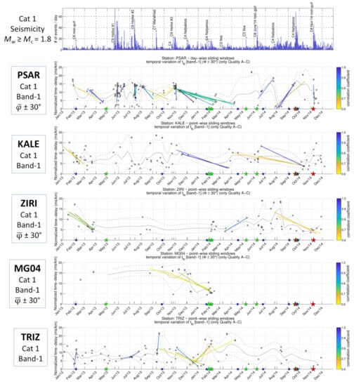
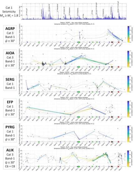
Figure 9.
(Top panel) Daily number of events from Cat1 with Mw ≥ Mc = 1.8. The initiation time of specific sequences is marked by labels (see also Figure 4). (Lower panels) Examples of tn measurements (circles) from several stations (station code in the box on the left) with respect to origin time. The solid gray line represents the 3-point moving average and the dashed gray line the respective ±1σ range as a measure of uncertainty. Coloured straight lines are derived from linear regressions, performed on sliding windows for various window lengths (see text for details), with colours corresponding to the correlation coefficient (≥0.6). The station code, catalogue number, band and other applied filters are indicated in the box on the left of each panel. The occurrence of major events is marked by stars at the bottom of each diagram (red: Mw ≥ 4.5, green: 4.0 ≤ Mw < 4.5, blue: 3.6 ≤ Mw < 4.0).
4. Discussion
4.1. Spatial Distribution of Seismicity and Possible Active Faults
The high-resolution hypocentral distribution of the present study reveals that the seismic activity is mostly concentrated in a ~2-km-thick, low-angle-dipping layer below the gulf, mainly between depths of 7 and 10 km. This is composed of distinct clusters associated with planar structures protruding towards shallower depths (see also Figure A5 and the interactive figure of File S1 in the Supplementary Material). Focal mechanisms (Figure 4 and Table 1) indicate that these clusters are related with normal faults of moderate dip angle. A connection of structures at depth to mapped faults at the surface is not always straightforward, either due to the activation of blind faults, rooting at the fragmented seismogenic layer, or to focal depth uncertainties and biases.
The latter case is important, as some systematic differences at hypocentral depths can be observed when compared to other studies. For example, [9] presented relocated seismicity of the period 2000–2015 in the WGoC using data from the CRL network, with focal depths mainly in the range of 6–8 km. Although in the northern part the focal depths of Cat1 are similar to those of [9], a deviation is observed in the southern and western parts of the study area, with absolute locations of our catalogue being 2–4 km deeper. This is likely a bias introduced by the inclusion of HUSN stations at epicentral distances further than 30 km, to better constrain epicenters near the margins of the local network, particularly towards the western part. The use of stations at distances up to 30 km tends to pull hypocenters towards shallower depths, especially at the southern part below Aigion, but also increases scattering in the distribution of epicenters. As a result, the foci in the present study are more clustered, but likely at the cost of a 1–2 km offset in absolute depths. The 2013 Helike swarm is an exception to this, as it has been separately processed using similar data, stations and velocity model as in [6], but considering it as a whole spatial group rather than on a sub-cluster level.
Concerning the larger events of the dataset, the 8 June 2014 event exhibits nearly E-W normal faulting (Table 1). [9] related this event with the south-dipping Trizonia fault. However, as observed in cross-section b1-b2 (Figure 4), this cluster of aftershocks seems to be consistent with a north-dipping structure that is likely associated with the Aigion-Selianitika fault system (GRIS503 in [14]; Figure S20) in group #8. As highlighted by [9], this earthquake seems to have also triggered seismicity to antithetic structures, sub-parallel to the Trizonia fault. Furthermore, its activity likely spreads eastwards to the Fasouleika segment, in group #6, particularly by the end of July 2014, in an opposite direction to what was observed in 2003–2004 [5].
Another significant event during the study period is the 21 September 2014 earthquake, which has been estimated at Mw = 4.6 (Mw = 4.9 from MT at NKUA and GI-NOA; Table 1). This event triggered aftershocks at the westernmost part of the 2014 Nafpaktos-Psathopyrgos swarm (group #4). Activity in this part of the WGoC has been related with the junction between the Rion-Patras fault zone, dipping NW and having a dextral strike-slip component, and the Psathopyrgos north-dipping normal fault [9]. The focal mechanism for this event suggests E-W to WSW-ENE normal faulting (strike = 254°, dip = 40°). Although the cross-section a1-a2 in Figure 4 is oblique to the focal mechanism, the hypocentral distribution shows a better fit with a NW-dipping plane. The 21 September 2014 event seems to coincide with the down-dip extension of the Ano Kastritsi fault. The triggered aftershocks, however, could have been spread to another structure, such as the Panachaikon transfer-fault (Pt.f., Figure 1 and Figure 4; [30]), which is parallel to the Rion-Patras fault but further east. When surface faults and deeper structures associated with the seismicity of group #4 are viewed in the 3D space (Figure S24, File S1 in the Supplementary Material), it is observed that the down-dip extension of the Rion-Patras fault and Panachaikon transfer fault, with a typical 60° dip, intersect the hypocentral distribution. If the seismicity cloud is interpreted as a combination of two parallel NW-dipping structures at a high angle (as in Figure S24), it is plausible to associate it with those two faults on the surface.
The 7 November 2014 event was previously referred to as having Mw = 5.0 (e.g., [48]), following the MT calculated at NKUA. However, spectral fitting provided Mw = 4.8 for this event, which is closer to the value reported by GI-NOA MT inversion (Mw = 4.8) and [9] (Mw = 4.7). This event is relocated within group #6, with a spatial gap to its south, followed by a cluster of aftershocks. The hypocentral distribution of this group suggests activation of a north-dipping structure at a relatively low angle (25° for the north-dipping plane of the focal mechanism). The southern sub-clusters of group #6, taken as a whole, have an apparent dip of ~40°. Allowing for a ~2 km offset at depth and some degree of listricity, the activated structure is compatible with the west Helike fault. [9] related the activity at the southern part of group #6 with the Aigion fault, as their hypocenters reach depths shallower than 5 km. Considering that group #6 is composed of high-angle structures, when viewed in the 3D space (Figure S23, File S1 in the Supplementary Material) it seems plausible to partly relate the seismic activity of this group with the down-dip extensions of the w. Helike fault, the Aigion fault and the Fasouleika segment.
4.2. Physical Mechanisms for Earthquake Migration
The temporal evolution of seismicity in the WGoC during 2013–2014 presents a series of bursts with significant earthquake migration patterns. The most characteristic one was observed in the offshore region between Nafpaktos and Psathopyrgos (group #4), mainly during July–October 2014, with migration speed in the range of 0.13–0.18 km/day eastwards and ~0.07–0.12 km/day westwards (Figure S22c). The occurrence of the 21 September 2014 earthquake in the west produced an aftershock sequence that severely accelerated earthquake migration rates to over 1 km/day in its vicinity. Seismicity migration speeds of the order of 100 m/day are associated with fluid-driven seismicity, as observed in several cases in the WGoC (e.g., [4,5,6]). The speed of the triggering front, due to pore-pressure diffusion, depends on the distance from the fluid injection source (Equation (1)) and from the permeability k of the rock, embedded in D = Nk/η, with other factors being the poro-elastic modulus, N, and the pore-fluid dynamic viscosity, η [50]. On the other hand, earthquake migration rates of over 1 km/day (e.g., 0.1–1 km/h) are likely attributed to aseismic creep episodes (e.g., [52]). [65] have documented the case of a seismic swarm in Malamata, i.e., below station MALA (Figure 1), which exhibited a pattern of expanding seismicity at a rate of ~125 m/day. However, it was manifested as a series of intermittent bursts, with seismicity migration speeds of 2–10 km/day over a short duration and distance. This example indicates how fluid-driven seismicity can be combined with short-lived aseismic slip episodes.
We presented a long-range earthquake migration pattern, covering a ~32 km distance from Nafpaktos to Aigion over the course of ~15 months (Figure 6). Although this sequence evolved eastwards at an average speed of ~70 m/day, it progressed in a series of bursts involving events of moderate magnitude that triggered their own sub-sequences. This pattern is consistent with pore-fluid diffusion, evidenced by an expanding triggering front of hydraulic diffusivity D = 2.2 m2/s through an active patch of 11–12 km, delimited by a back-front of seismicity deficit (Figure 6). A similar pattern has been observed in 2011 in Oichalia, South Peloponnese, where, likewise, a swarm evolved southwards in a series of episodes associated with major events of NNW-SSE-oriented normal faults, within an active patch following a parabolic triggering front [66]. In that case, the hydraulic diffusivity was D = 1.1 m2/s, the active fault patch was ~8-km-long and it traveled a distance of ~10 km over 160 days, i.e., at an average speed of 63 m/day.
In addition, we estimated the mean squared distance (msd) of seismicity with time for the eastwards expanding seismic activity, enclosed within the active patch defined by the triggering- and back-fronts. The msd shows a step-like increase with time that can be approximated, overall, by a power-law function, with a diffusion exponent of a = 1.81 ± 0.17 that indicates super-diffusion. [60] studied separately the distinct seismic clusters occurring in the spatial groups #4, #6 and #8 (e.g., Figure A1, Figure A3 and Figure A4 in Appendix A), yielding diffusion exponents lower than 0.2 and sub-diffusion. However, herein we observe that if the seismic clusters are jointly studied on a larger scale, a much faster diffusive process is obtained that spans from the Rion strait in the west to offshore Aigion in the east (Figure 4, top). In terms of the CTRW theory, the overall super-diffusive process resembles a Lévy walk (e.g., [67]), with intermediate asymptotics having different exponents. High diffusion exponents, close to or greater than unity, are found in anomalous fluid transport processes in heterogeneous and fractured media [68]. Numerical simulations of fluid transport in heterogeneous fault zones also show anomalous diffusion with exponents greater than 1, as fluid flow is channeled in fractal fault zones with varying permeabilities [69]. In contrast, stress transfer effects due to subcritical crack growth or to cascading effects yield quite low diffusion exponents and sub-diffusion [57,58], most commonly observed in earthquake diffusion [49,60]. The super-diffusive behavior of seismicity reported herein may, thus, provide an additional indication of fluid overpressures.
Consequently, a candidate physical mechanism for the observed seismicity migration pattern in the offshore region of the WGoC during the ~15 months period may well correspond to an initial intrusion of overpressurized fluids from the area of Nafpaktos. In a fluid-saturated and critically stressed crust, fluid overpressures can reduce the effective normal stress along the active fault structures, triggering the observed seismicity offshore Nafpaktos during September–December 2013 (Figure S22b). Fluid diffusion along an E-W-oriented, permeable pathway, defined by the intersection of the active fault structures with the shallow-dipping seismogenic layer beneath the WGoC, may have caused the eastward migration of seismicity. This eventually activated the easternmost part of group #4 and the westernmost part of group #8 during January–February 2014, which included certain Mw > 3.8 events (Figure S22b, yellow colour). Increased stresses in this area trigger additional events towards the east during March–May 2014, until 8 June 2014, when the Mw = 4.3 earthquake occurred in group #8. The latter initiated an aftershock sequence, including several Mw ≥ 3.0 events in group #8 and eastwards in group #6 during July–October 2014. Seismic activity then culminated with an Mw = 4.8 event on 7 November 2014 in group #6, offshore Aigion, initiating an aftershock sequence that spread rapidly in an E-W direction and mostly south of the mainshock’s epicenter until the end of 2014 (Figure S22c).
The overall seismicity migration pattern is, thus, likely produced by a combination of fluid diffusion and stress transfer effects caused by the larger magnitude events. Enhanced permeabilities due to fluid flow in the area of group #4, followed by healing/sealing processes in the active faults (e.g., [70]), may have caused the deficit of the seismic activity, delimited by the back-front observed during March–June 2014 (Figure 6). In mid-July 2014, the seismic activity at group #4 increases again in the same area, as during September-December 2013, possibly triggered by another intrusion of overpressurized fluids. This resembles a conventional fault-valve behavior [71], in which the low-permeability Phyllade nappe below the shallow-dipping seismogenic layer acts as a cap for a deeper fluid reservoir evidenced by VP/VS anomalies [5,65,72,73]. A combination of fluid diffusion, aseismic creep, supported by fast earthquake migration speeds, and stress transfer effects caused by the Mw > 4 events during September 2014, may have caused the bilateral migration of seismicity that was observed offshore Nafpaktos during July–October 2014.
4.3. Seismic Anisotropy in the WGoC
The comprehensive dataset of shear-wave splitting parameters of the present study may provide evidence regarding changes in the local stress field, fluid diffusion or saturation that can affect the anisotropic properties of the medium. Previous upper-crust anisotropy studies in the WGoC have focused in the 2010 Efpalio sequence [74], the 2013 Helike swarm [75] and the November 2014 sequence [48]. Their findings indicate that the fast shear-wave polarization directions are consistent with the maximum horizontal stress component, σHmax (e.g., [76]), which is in a WNW-ESE direction, parallel to the strike of major normal faults. Herein, the obtained mean φ directions are collectively presented in Figure 10. Notably, the results of the automatic analysis are, on average, consistent with those of [48,75], who performed manual SWS measurements through visual inspection of polarigrams and hodograms. In the following, the presented average values of the SWS parameters are from measurements of Cat1, unless specified otherwise. These measurements concern the volume between the sources and the receiver as sampled by the seismic ray-paths, whose length is used for the normalization of the time-delays.
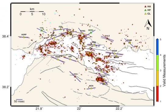
Figure 10.
Map of candidate events for SWS measurements from Cat1 (manual only) in the WGoC during 2013–2014. Blue lines represent the average fast S-wave polarization direction, φ (orientation), and time-delay, td (length), at the respective station (triangle, coloured according to network code). Coloured circles correspond to events with valid SWS measurements (grade A to C), whereas gray circles are events without valid measurements (only D, E or null). Red lines depict the respective mean polarization direction derived from Cat3 (see also Figure S18 in the Supplementary Material).
In addition, we provide SWS measurements for stations in the WGoC that were not analyzed previously, such as AIOA, HELI and TEME in the south, as well as PANR and PSAM (Cat3 only) in the north. Station TEME presents a NW-SE direction (145.1° ± 16.3°), which does not appear to be consistent with σHmax or the strike of local structures, but is similar to that of LAKA ( = 134.7° ± 5.9°), to the west. On the other hand, HELI, a temporary station installed to record the 2013 Helike sequence [6], exhibits a WSW-ENE direction (77.6° ± 11.6°) that is similar to that of the neighboring AIOA station to the south ( = 79.4° ± 7.7°). However, the value at station HELI deviates from the direction indicated by the largest percentage of φ measurements, which is ~E-W, as can be observed from the respective rose diagram (Figure S16), with a secondary SSW-NNE φ direction. Stations AIOA and HELI are related with the epicentral regions of the 2001 Agios Ioannis [4,49] and 2013 Helike [6,48] swarms, both being either directly or partially related with the re-activation of older structures, which are not optimally oriented to the present-day stress-field. Specifically, the 2001 Agios Ioannis swarm has been attributed to the Kerinitis fault (Figure 1), with a strike that is SW-NE to WSW-ENE, consistent with measured at AIOA and HELI. The direction measured at TEME, however, is almost perpendicular to that of its neighboring station HELI, although the stations are located in close vicinity (~2 km apart).
In the north, the directions at stations TRIZ, PSAR and PSAM are nearly E-W, consistent with both σHmax and fault orientations. An important difference was previously observed at stations PYRG and SERG, with oriented SW-NE, a deviation that was attributed to the strike of local structures [48,75], particularly to mapped offshore faults with significant strike-slip component (e.g., [17]). In the present study, however, station PYRG exhibits a much different NW-SE direction in Cat1 (142.2°), albeit with a very significant error (±41.6°). On the other hand, in Cat3, where more measurements are available, station PYRG shows a more E-W-oriented , although with a still large uncertainty (102.4° ± 29.6°). This is due to the significant scatter in φ measurements (Figure S16), while a secondary φ maximum at a SW-NE direction, that would be in agreement with previous studies, is also observed. The existence of two groups of φ measurements at stations PYRG and HELI indicates either a strong spatial dependence or that shear-waves propagate through two distinct media with different anisotropic properties [21,77,78].
The measurements at the neighboring station SERG are very consistent, with = 58.4° ± 7.5°. Further west, stations EFP and MALA present an E-W to WSW-ENE direction, consistent with previous findings [48,75]. Regarding the Magoula seismic array, station MG00, with = 82.2° ± 7.5°, is in agreement with the results of [48]. Other stations of the array present variability in their values, ranging between 60.7° and 106.3° (Figure S16). Station MG06, however, with more consistent measurements and smaller error, yields = 85.6° ± 8.9°, in general agreement with MG00. The WSW-ENE orientation at station MALA (68.1° ± 11.0°) appears as a smooth transition in relation to the respective at the neighboring stations EFP and MG00, and is also consistent with the strike of the Nafpaktos fault. Observations of at stations MALA and SERG favor the existence of structurally controlled anisotropy [41,79,80]. Further west, stations AGRP and VVK present an E-W to WNW-ESE direction, more consistent with σHmax [48,75]. Notably, in the WGoC the mapped faults’ strike changes from E-W in the north to WNW-ESE in the south, the latter being in agreement with measured at stations ROD3, ZIRI and ALIK. Stations TEME and LAKA show a more pronounced NW-SE direction, consistent with the results of [81], regarding the latter station.
In addition, we investigated patterns of changes in the normalized time-delays, tn, between the fast and slow split shear-waves, possibly associated with the observed evolution of seismicity in the WGoC. We point out three cases of linear decrease in tn values, which could be related to stress-relaxation due to microcrack coalescence. The first is associated with the period before the occurrence of the 2013 Helike swarm, between January and May 2013. The second was observed between November 2013 and January 2014, i.e., near the beginning of the fluid-driven, long-range seismic sequence. In particular, a cluster within group #4 occurred in late November 2013, while mid- to late December marks the beginning of the back-front, or the end of the “injection” period (~120 days). The pore-pressure pulse then travels at a speed of ~0.13 km/day until January-February 2014 at the eastern end of group #4 and part of groups #6 and #8 (Y = 23–30 km in Figure 6). This epicentral area north of the Psathopyrgos fault has been previously proposed as the source of a strain transient event of equivalent Mw = 5.3 that occurred on 3 December 2002 and was detected by a dilatometer at Trizonia Island [82]. To the east of this likely creeping fault patch, there is an area where larger events have occurred, including the recent Mw = 5.3 event of 17 February 2021 (Figure 1; [83]). The last decreasing tn pattern was observed during the months before the 7 November 2014 event. A similar decrease pattern has been reported by [48] at stations ZIRI and SERG during that period, while at ROD3 station both an increase and a decrease period were identified; a pattern that could possibly be considered as precursory behavior.
Regarding the upper-crust anisotropy in the WGoC, a future goal would be the identification of the depth of the anisotropic layer. However, this would require recordings at the same site both on the surface and at various depths. Unfortunately, there are currently no such stations in the study region. Thus, we consider the whole medium between the hypocenter and the station as anisotropic. Another prospective step is the computation of the spatial averaging of the fast shear-wave polarization direction at the surface [84], in order to determine changes of φ at areas where no seismological stations are available, but this is beyond the scope of the present study.
5. Conclusions
To summarize, the presented results highlight the complex seismicity patterns that were observed during a two-year period in the Western Gulf of Corinth. The high resolution earthquake catalogue enabled the recognition of the activated structures at depth and their possible relation to mapped faults on the surface. The detailed spatiotemporal evolution of seismicity revealed interactions between neighboring structures via a migrating active patch, likely associated with increased pore-pressure. Measurements of shear-wave parameters were performed on a larger scale than ever before in the WGoC through an automated procedure, validating previous results from manual analysis and providing new information at different sites or study periods. The seismic monitoring of the WGoC over the past 20 years has been providing valuable information on the manners with which seismicity is evolved, driven by fluids that propagate through the microfracture network, enabling aseismic creep, triggering swarms and mainshock-aftershock sequences on their way. The high deformation rate in this part of Central Greece ensures that such patterns will continue to emerge and may eventually lead to significant and destructive events. The understanding of the dynamics of seismicity may therefore play an important role for the assessment of seismic hazard in the area.
Supplementary Materials
The following are available online at https://www.mdpi.com/article/10.3390/app11146573/s1, Section S1: Location/Relocation statistics for Catalogue 1, Section S2: Seismic moment measurements, Section S3: Automatic picking for Catalogue 2, Section S4: Additional tables and figures, File S1: 3D Interactive Matlab Figure, Dataset D1: Catalogue of seismicity, Dataset D2: Anisotropy measurements, Table S1: Absolute location error and other statistics per spatial group (see Figure 2) for the seismicity of 2013–2014 (Catalogue 1) in the Western Gulf of Corinth (WGoC). Table after [60], Table S2: Statistics of the station jack-knife test for the relocation robustness per spatial group of the 2013–2014 seismicity in the WGoC, with dx, dy and dz values representing perturbations from the true relocated hypocenter. The 95% confidence interval ellipse major semi-axis length refers to the horizontal ellipses of Figure S2, as estimated for each whole spatial group, Table S3: Mean values of SWS parameters and their respective errors per station for valid measurements (grade A-C) of Catalogue 3. Stations with additional data from Catalogue 2 are marked with a star (*) next to their station code. Errors correspond to the 95% c.i, whereas and are the typical error of mean. N is the number of valid measurements per station. The first line in bold corresponds to all valid measurements of Cat3, Figure S1: Location statistics for Catalogue 1. (a) RMS travel-time error, (b) horizontal (ERX, ERY) and vertical (ERZ) location uncertainties, taking into account an average arrival-time reading error of 0.13sec, (c) number of phases with non-zero true weight, (d) focal depth (including relocated hypocenters with HypoDD), (e) azimuthal gap and (f) epicentral distance of the nearest station with arrival-time data. Absolute location errors and RMS travel-time errors are nominal values reported by HypoInverse, Figure S2: Distribution of 95% c.i. ellipses for epicentral perturbations derived by the station jack-knife test for the robustness of the relocation procedure, Figure S3: Cross-sections a1-a2 to c1-c2 (Figure S2) with vertical and horizontal bars representing the vertical and horizontal (square root of dx2 + dy2) average perturbation of each hypocenter, respectively, derived by the application of the station jack-knife test for the robustness of the relocation procedure, Figure S4. Example of seismic moment calculation by spectral fitting for the 15 July 2013, Mw = 3.8 event on the short-period station TEME (top) before residual correction and (bottom) after residual correction. The blue and dashed red lines correspond to signal and noise spectra, respectively. The S-wave window is also presented in the inset panel at the bottom-left, Figure S5. Examples of spectral moment fit residual distribution (left) for the short-period station TEME and (right) for the broad-band station KALE, Figure S6. Same as Figure S4, but for the recording of the 15 July 2013, Mw = 3.8 event on the broad-band station KALE (top) before residual correction and (bottom) after residual correction, Figure S7. (a) Map of automatic CRL locations for 2013–2014. (b) Map of automatic locations for Catalogue 2 in this study, after removal of regional events/low quality locations and with the combined application of multiple-window AIC and template-matching picking methods and (c) same as (b), but after the removal of average travel-time residuals, as a rough application of station corrections for groups 4–9, Figure S8. Example of an automatic pick on the P-wave using the multiple-window AR-AIC method. (Top) The Z component in the maximum length window, along with the approximate arrival (dashed black line) and the final pick on the P-wave (red). (Bottom) AIC function for different components (red = Z, green = N-S, blue = E-W) calculated in multiple different window lengths. For this visualization, the maximum of the AIC functions has been subtracted and their values are normalized in proportion to the window length. (Left) Waveform windows for the three components, with the same colours as in the bottom panel. The dashed rectangle shows the maximum length window (top panel), Figure S9. Same as Figure S8, but for an automatic pick on an S-wave, Figure S10. Example of a rejected automatic pick due to excess noise resulting in scattered AIC minima, Figure S11. Example of automatic picks on P- and S-waves using the template matching method. The top waveform (black) belongs to the target event (to be picked). Red and green waveforms correspond to the best matching P- and S-wave templates, respectively. Arrival-time picks shown as vertical lines on the templates, with their colour corresponding to their correlation coefficient (CC). The final P- and S-wave pick is marked on the target waveform with a down-pointing arrow at the top of a red and green thick line, respectively. Available picks from more templates (with lower CC) are also shown on the target waveform, Figure S12. Same as Figure S11, but for a different target waveform, Figure S13. (Top) Map of relocated seismicity for 2013–2014 in the WGoC. Colours correspond to the 9 spatial groups in which the dataset was divided, along with the “miscellaneous” group #10 (gray). Beachballs depict the focal mechanisms of major events (Table 1). (Bottom panels) Vertical cross-sections a1–a2 to p1–p2, drawn in a N10°E direction, corresponding to the dashed rectangles shown on the map (top). Beachballs depict the far hemisphere projections of focal mechanisms for major events. Black dashed lines at the top of the cross-sections indicate the position of mapped active faults with inferred extension at a 60° dip. For mapped faults’ names refer to Figure 1, Figure S14. (Top) Map of relocated seismicity for 2013–2014 in the WGoC. Colours correspond to the 9 spatial groups in which the dataset was divided, along with the “miscellaneous” group #10 (gray). Beachballs depict the focal mechanisms of major events (Table 1). (Bottom panels) vertical cross-sections a1–a2 to e1–e2, drawn in a N315°E direction, corresponding to the dashed rectangles shown on the map (top). Beachballs depict the far hemisphere projections of focal mechanisms for major events. Black dashed lines at the top of the cross-sections indicate the position of mapped active faults with inferred extension at a 60° dip. For mapped faults’ names refer to Figure 1, Figure S15. (Top) Map of relocated seismicity for 2013–2014 in the WGoC. Colours correspond to the 9 spatial groups in which the dataset was divided, along with the “miscellaneous” group #10 (gray). (Bottom panel) Vertical cross-section A-B, drawn in a N100°E direction, corresponding to the dashed rectangle shown on the map (top). The y-axis of the cross-section is exaggerated. The Kamarai fault zone (f.z.) comprises Lambiri, Selianitika and Fasouleika faults, Figure S16: Rose diagrams of the distribution of the fast shear-wave polarization angle φ for valid measurements with grade A (best) to C (acceptable) from Catalogue 1 (only manually located/relocated events) per station (station code shown on top of each diagram). Colours correspond to the respective normalized time-delay tn. The red arrows indicate the average φ direction, Figure S17: Rose diagrams of the distribution of the polarization angle φ for null measurements (where φ is in the range of p ± 10° or (p + 90°)±10°) from Catalogue 1 (only manually located/relocated events) per station (station code shown on top of each diagram). Colours correspond to the respective normalized time-delay tn. The red arrows indicate the average φ direction of null measurements, Figure S18. Map of candidate events for SWS measurements from Cat3 (manual and automatic) in the WGoC during 2013–2014. Blue lines represent the average fast S-wave polarization direction, φ (orientation), and time-delay, td (length), at the respective station (triangle, coloured according to network code). Coloured circles correspond to events with valid SWS measurements (grade A to C), whereas gray circles are events without valid measurements (only D, E or null), Figure S19. Gutenberg-richter law for the seismicity of Catalogue 1. Mc = 1.8 is the magnitude of completeness. The b-value is calculated as 1.235±0.015 from linear regression (correlation coefficient R = −0.998) or bMLE = 1.185 from the maximum likelihood method, Figure S20. Composite Seismogenic Sources (orange) and Individual Seismogenic Sources (yellow) from the Greek Database of Seismogenic Sources (GreDaSS, [14]) in the WGoC area, mentioned in the main text. GRCS441: Trikorfo source, associated with Trikorfo and Sergoula faults, GRCS500: South Corinth Gulf source, associated with Sela, Lakka, w. Helike and e. Helike faults, GRCS524: Mamoussia source, associated with Pirgaki and Mamoussia faults, GRIS502: west Helike fault source, also associated with Lakka fault, GRIS503: Aigion fault source, also associated with Fasouleika and Selianitika faults, Figure S21. Schematic representation of Band-1 and Band-2 zones, modified after [85]. The receiver at the surface is marked with S. The ABCD plane of vertically aligned microcracks is oriented towards the mean fast shear-wave polarization direction, Φ. Band-1 contains seismic rays traveling towards the seismic station at directions contained within the solid angle EFGH-to-S (blue),at angles between 15° and 45° (shear-wave window) on either side of the crack-plane. Band-2 contains seismic rays that travel within the solid angle ADEHG-to-S (red) towards the seismic station, i.e., within ±15° from the crack-plane, Figure S22. Maps of the temporal evolution of the 2013–2014 sequence in the WGoC (Catalogue 1, all spatial groups except #3 and #10). The colours represent relative origin time (see labels on the colour-scale of each panel). (a) January – August 2013: the map shows sporadic activity inside the gulf, with the most significant cluster being the 2013 Helike sequence. (b) September 2013 – 14 July 2014: several clusters were observed at the western part of group #4, with activity going back and forth as shown with the red arrows. The dashed red ellipse shows a possible source of fluid injection. The black arrows show the direction (N100°E) and speed of seismicity migration or inferred fluid diffusion (see Figure 5). Seismicity gradually migrated eastwards at ~0.13km/day, activating the clusters with yellow colour (days 380–400). Fluid diffusion at a rate of 0.04km/day towards N100°E precedes the triggering of the June 2014 sequence (dark blue), during which seismicity migration at 0.75 km/day was observed within the cluster (see also Figure A2). (c) 15 July – December 2014: bilateral seismicity migration observed in the spatial group #4, starting from the region marked with the red dashed ellipse (same as in panel b). Seismicity migration at a speed of 0.05km/day towards N100°E between groups #8 and #6 is marked with a black arrow. The 7 November 2014 Mw = 4.8 event (green star) triggers seismicity mostly southwards, Figure S23. Annotated snapshot of the interactive 3D figure (File S1), showing the spatial group #6 and associated structure planes, along with selected surface fault planes (gray) extended downwards to the depth of 8 km at a 60° dip. The view is towards west. No vertical exaggeration has been applied, Figure S24. Annotated snapshot of the interactive 3D figure (File S1), showing the spatial groups #4 (green) and #5 (orange) and proposed associated structure planes. Selected surface fault planes (gray) are extended downwards to the depth of 8 km at a 60° dip. The view is towards north-east. No vertical exaggeration has been applied, Figure S25. Annotated snapshot of the interactive 3D figure (File S1), showing the 2013 Helike swarm (spatial group #9) and associated structure planes that were activated (blue). The surface fault planes (gray) of Pirgaki and Kerinitis faults are shown in gray. The view is downwards and towards NNE. Although the swarm is mainly associated with the north-dipping Pirgaki fault, it also contained events with oblique-normal focal mechanisms, likely related to NW-dipping structures sub-parallel to Kerinitis fault [6].
Author Contributions
Conceptualization, G.K., V.K., G.M. and F.V.; methodology, V.K., G.K., G.M. and F.V.; software, V.K., G.K. and G.M.; validation, V.K. and G.K.; formal analysis, V.K. and G.K.; investigation, V.K., G.K, G.M. and F.V.; resources, V.K.; data curation, V.K.; writing—original draft preparation, V.K.; writing—review and editing, V.K., G.M., G.K. and F.V.; visualization, V.K. and G.M.; supervision, G.K. and F.V.; project administration, G.K.; funding acquisition, G.K. and F.V. All authors have read and agreed to the published version of the manuscript.
Funding
The present research is co-financed by Greece and the European Union (European Social Fund- ESF) through the Operational Programme «Human Resources Development, Education and Lifelong Learning 2014–2020» in the context of the project “The role of fluids in the seismicity of the Western Gulf of Corinth (Greece)” (MIS 5048127).
Institutional Review Board Statement
Not applicable.
Informed Consent Statement
Not applicable.
Data Availability Statement
The seismicity catalogue (Dataset D1) and shear-wave splitting measurements (Dataset D2) are available in the Supplementary Material. The CRL automatic catalogue is available at http://ephesite.ens.fr/~eworm/ (accessed on 14 July 2021) Waveform data are publicly available for CRL stations at RESIF (http://seismology.resif.fr/ (accessed on 14 July 2021)), and for HUSN stations at the EIDA node of NOA (http://eida.gein.noa.gr/ (accessed on 14 July 2021)).
Acknowledgments
We would like to thank the personnel of the Hellenic Unified Seismological Network (http://eida.gein.noa.gr/) (accessed on 14 July 2021) and the Corinth Rift Laboratory Network (https://doi.org/10.15778/RESIF.CL (accessed on 14 July 2021)) for the installation and operation of the stations used in the current article. We thank Ioannis Spingos for discussions and support with the application of the Pytheas software. Rose diagrams were constructed using the “Wind Rose” MATLAB routine [86]. Maps were drawn with the Generic Mapping Tools (GMT) software [87]. Shear-wave splitting measurements were performed with the Pytheas software [40].
Conflicts of Interest
The authors declare no conflict of interest.
Appendix A. Additional Figures
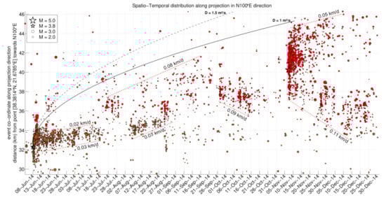
Figure A1.
Spatiotemporal evolution of the June-November 2014 mid-gulf sequence (groups #8 and #6). Dashed red lines indicate linear seismicity migration patterns, with speed presented in km/day. Parabolic triggering fronts are drawn for reference with D = 1.0 m2/s (solid) and D = 1.5 m2/s (dashed) black lines.
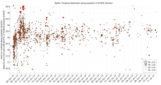
Figure A2.
Spatiotemporal evolution of the June 2014 mid-gulf sequence (group #8), between 8 June and 12 July 2014. Dashed red lines indicate linear seismicity migration patterns, with speed presented in km/day.
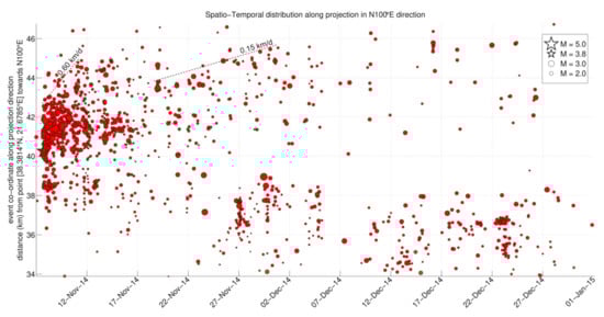
Figure A3.
Spatiotemporal evolution of the November 2014 mid-gulf sequence (group #6), between 8 November and 31 December 2014. Dashed lines indicate linear seismicity migration patterns, with speed presented in km/day.
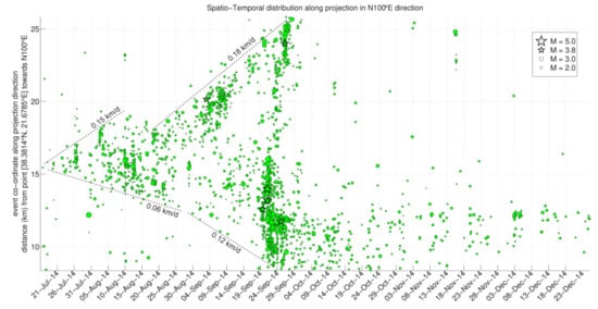
Figure A4.
Spatiotemporal evolution of the Nafpaktos 2014 swarm (group #4) in the period of July–December 2014. Dashed lines indicate linear seismicity migration patterns, with speed presented in km/day.
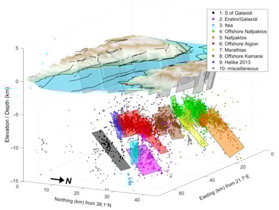
Figure A5.
Annotated snapshot of the interactive 3D figure provided in the Supplementary Material (File S1), showing the 2013−2014 seismicity in the WGoC along with surface faults and activated structures at depth associated with each spatial group. The view is towards south-west. The vertical axis is exaggerated by ×2.
References
- Avallone, A.; Briole, P.; Agatza-Balodimou, A.M.; Billiris, H.; Charade, O.; Mitsakaki, C.; Nercessian, A.; Papazissi, K.; Paradisis, D.; Veis, G. Analysis of eleven years of deformation measured by GPS in the Corinth Rift Laboratory area. C. R. Geosci. 2004, 336, 301–311. [Google Scholar] [CrossRef] [Green Version]
- Briole, P.; Ganas, A.; Elias, P.; Dimitrov, D. The GPS velocity field of the Aegean. New observations, contribution of the earthquakes, crustal blocks model. Geophys. J. Int. 2021, 226, 468–492. [Google Scholar] [CrossRef]
- Lyon-Caen, H.; Papadimitriou, P.; Deschamps, A.; Bernard, P.; Makropoulos, K.; Pacchiani, F.; Patau, G. First results of the CRLN seismic network in the western Corinth Rift: Evidence for old-fault reactivation. C. R. Geosci. 2004, 336, 343–351. [Google Scholar] [CrossRef] [Green Version]
- Pacchiani, F.; Lyon-Caen, H. Geometry and spatio-temporal evolution of the 2001 Agios Ioanis earthquake swarm (Corinth Rift, Greece). Geophys. J. Int. 2010, 180, 59–72. [Google Scholar] [CrossRef]
- Duverger, C.; Godano, M.; Bernard, P.; Lyon-Caen, H.; Lambotte, S. The 2003–2004 seismic swarm in the western Corinth rift: Evidence for a multiscale pore pressure diffusion process along a permeable fault system. Geophys. Res. Lett. 2015, 42, 7374–7382. [Google Scholar] [CrossRef]
- Kapetanidis, V.; Deschamps, A.; Papadimitriou, P.; Matrullo, E.; Karakonstantis, A.; Bozionelos, G.; Kaviris, G.; Serpetsidaki, A.; Lyon-Caen, H.; Voulgaris, N.; et al. The 2013 earthquake swarm in Helike, Greece: Seismic activity at the root of old normal faults. Geophys. J. Int. 2015, 202, 2044–2073. [Google Scholar] [CrossRef] [Green Version]
- Mesimeri, M.; Karakostas, V.; Papadimitriou, E.; Schaff, D.; Tsaklidis, G. Spatio-temporal properties and evolution of the 2013 Aigion earthquake swarm (Corinth Gulf, Greece). J. Seismol. 2016, 20, 595–614. [Google Scholar] [CrossRef]
- Lambotte, S.; Lyon-Caen, H.; Bernard, P.; Deschamps, A.; Patau, G.; Nercessian, A.; Pacchiani, F.; Bourouis, S.; Drilleau, M.; Adamova, P. Reassessment of the rifting process in the Western Corinth Rift from relocated seismicity. Geophys. J. Int. 2014, 197, 1822–1844. [Google Scholar] [CrossRef]
- Duverger, C.; Lambotte, S.; Bernard, P.; Lyon-Caen, H.; Deschamps, A.; Nercessian, A. Dynamics of microseismicity and its relationship with the active structures in the western Corinth Rift (Greece). Geophys. J. Int. 2018, 215, 196–221. [Google Scholar] [CrossRef]
- Mesimeri, M.; Karakostas, V.; Papadimitriou, E.; Tsaklidis, G. Characteristics of earthquake clusters: Application to western Corinth Gulf (Greece). Tectonophysics 2019, 767, 228160. [Google Scholar] [CrossRef]
- Bernard, P.; Briole, P.; Meyer, B.; Gomez, J.; Tiberi, C.; Berge, C.; Cattin, R.; Hatzfeld, D.; Lachet, C.; Lebrun, B.; et al. The Ms = 6.2, June 15, 1995 Aigion earthquake (Greece): Evidence for low-angle normal faulting in the Corinth rift. J. Seismol. 1997, 1, 131–150. [Google Scholar] [CrossRef]
- Armijo, R.; Meyer, B.; King, G.C.P.; Rigo, A.; Papanastassiou, D. Quaternary evolution of the Corinth Rift and its implications for the Late Cenozoic evolution of the Aegean. Geophys. J. Int. 1996, 126, 11–53. [Google Scholar] [CrossRef] [Green Version]
- Michas, G.; Vallianatos, F.; Sammonds, P. Statistical mechanics and scaling of fault populations with increasing strain in the Corinth Rift. Earth Planet. Sci. Lett. 2015, 431, 150–163. [Google Scholar] [CrossRef]
- Caputo, R.; Pavlides, S. The Greek Database of Seismogenic Sources (GreDaSS), version 2.0.0: A compilation of potential seismogenic sources (Mw > 5.5) in the Aegean Region. 2013. Available online: https://iris.unife.it/handle/11392/1849303#.YO4280y-tPY (accessed on 14 July 2021).
- Valkaniotis, S. Correlation between Neotectonic Structures and Seismicity in the Broader Area of Gulf of Corinth (Central Greece). Ph.D. Thesis, Aristotle University of Thessaloniki, Thessaloniki, Greece, 2009. [Google Scholar]
- Bell, R.E.; McNeill, L.C.; Bull, J.M.; Henstock, T.J.; Collier, R.E.L.; Leeder, M.R. Fault architecture, basin structure and evolution of the Gulf of Corinth rift, central Greece. Basin Res. 2009, 21, 824–855. [Google Scholar] [CrossRef]
- Beckers, A.; Hubert-Ferrari, A.; Beck, C.; Bodeux, S.; Tripsanas, E.; Sakellariou, D.; De Batist, M. Active faulting at the western tip of the Gulf of Corinth, Greece, from high-resolution seismic data. Mar. Geol. 2015, 360, 55–69. [Google Scholar] [CrossRef] [Green Version]
- Crampin, S. Seismic-wave propagation through a cracked solid: Polarization as a possible dilatancy diagnostic. Geophys. J. Int. 1978, 53, 467–496. [Google Scholar] [CrossRef] [Green Version]
- Crampin, S.; Zatsepin, S.V. Modelling the compliance of crustal rock-II. Response to temporal changes before earthquakes. Geophys. J. Int. 1997, 129, 495–506. [Google Scholar] [CrossRef] [Green Version]
- Zatsepin, S.V.; Crampin, S. Modelling the compliance of crustal rock-I. Response of shear-wave splitting to differential stress. Geophys. J. Int. 1997, 129, 477–494. [Google Scholar] [CrossRef] [Green Version]
- Sibson, R.H. Crustal stress, faulting and fluid flow. Geol. Soc. London Spec. Publ. 1994, 78, 69–84. [Google Scholar] [CrossRef]
- Papadimitriou, P.; Kaviris, G.; Makropoulos, K. Evidence of shear-wave splitting in the eastern Corinthian Gulf (Greece). Phys. Earth Planet. Int. 1999, 114, 3–13. [Google Scholar] [CrossRef]
- Kaviris, G. Study of Seismic Source Properties of the Eastern Gulf of Corinth. Ph.D. Thesis, National and Kapodistrian University of Athens, Athens, Greece, 2003. (In Greek). [Google Scholar]
- Kaviris, G.; Kapetanidis, V.; Kravvariti, P.; Karakonstantis, A.; Bozionelos, G.; Papadimitriou, P.; Voulgaris, N.; Makropoulos, K. Anisotropy study in Villia (E. Corinth Gulf, Greece). In Proceedings of the Second European Conference on Earthquake Engineering and Seismology(2ECEES), Istanbul, Turkey, 25–29 August 2014. [Google Scholar]
- Kaviris, G.; Papadimitriou, P.; Kravvariti, P.; Kapetanidis, V.; Karakonstantis, A.; Voulgaris, N.; Makropoulos, K. A detailed seismic anisotropy study during the 2011–2012 unrest period in the Santorini Volcanic Complex. Phys. Earth Planet. Int. 2015, 238, 51–88. [Google Scholar] [CrossRef]
- Kaviris, G.; Spingos, I.; Millas, C.; Kapetanidis, V.; Fountoulakis, I.; Papadimitriou, P.; Voulgaris, N.; Drakatos, G. Effects of the January 2018 seismic sequence on shear-wave splitting in the upper crust of Marathon (NE Attica, Greece). Phys. Earth Planet. Int. 2018, 285, 45–58. [Google Scholar] [CrossRef]
- Kaviris, G.; Spingos, I.; Karakostas, V.; Papadimitriou, E.; Tsapanos, T. Shear-wave splitting properties of the upper crust, during the 2013–2014 seismic crisis, in the CO2-rich field of Florina Basin, Greece. Phys. Earth Planet. Int. 2020, 303, 106503. [Google Scholar] [CrossRef]
- Bouin, M.-P.; Téllez, J.; Bernard, P. Seismic anisotropy around the Gulf of Corinth, Greece, deduced from three-component seismograms of local earthquakes and its relationship with crustal strain. J. Geophys. Res. Solid Earth 1996, 101, 5797–5811. [Google Scholar] [CrossRef]
- Sokos, E.; Zahradnik, J.; Kiratzi, A.; Janský, J.; Gallovic, F.; Novotny, O.; Kostelecký, J.; Serpetsidaki, A.; Tselentis, G.-A. The January 2010 Efpalio earthquake sequence in the western Corinth Gulf (Greece). Tectonophysics 2012, 530–531, 299–309. [Google Scholar] [CrossRef]
- Flotté, N.; Sorel, D.; Müller, C.; Tensi, J. Along strike changes in the structural evolution over a brittle detachment fault: Example of the Pleistocene Corinth–Patras rift (Greece). Tectonophysics 2005, 403, 77–94. [Google Scholar] [CrossRef]
- Evangelidis, C.P.; Triantafyllis, N.; Samios, M.; Boukouras, K.; Kontakos, K.; Ktenidou, O.-J.; Fountoulakis, I.; Kalogeras, I.; Melis, N.S.; Galanis, O.; et al. Seismic Waveform Data from Greece and Cyprus: Integration, Archival, and Open Access. Seismol. Res. Lett. 2021, 92, 1672–1684. [Google Scholar] [CrossRef]
- Klein, F.W. User’s Guide to HYPOINVERSE-2000, a Fortran Program to Solve for Earthquake Locations and Magnitudes; Open-File Report 2002-171; U.S. Geological Survey: Menlo Park, CA, USA, 2002; pp. 2002–2171. [Google Scholar] [CrossRef] [Green Version]
- Rigo, A.; Lyon-Caen, H.; Armijo, R.; Deschamps, A.; Hatzfeld, D.; Makropoulos, K.; Papadimitriou, P.; Kassaras, I. A microseismic study in the western part of the Gulf of Corinth (Greece): Implications for large-scale normal faulting mechanisms. Geophys. J. Int. 1996, 126, 663–688. [Google Scholar] [CrossRef] [Green Version]
- Ward, J.H. Hierarchical Grouping to Optimize an Objective Function. J. Am. Stat. Assoc. 1963, 58, 236–244. [Google Scholar] [CrossRef]
- Kapetanidis, V. Spatiotemporal Patterns of Microseismicity for the Identification of Active Fault Structures Using Seismic Waveform Cross-Correlation and Double-Difference Relocation. Ph.D. Thesis, University of Athens, Athens, Greece, 2017. [Google Scholar]
- Waldhauser, F. hypoDD—A Program to Compute Double-Difference Hypocenter Locations; Open File Report 01-113; U.S. Geological Survey: Menlo Park, CA, USA, 2001; 25p. [Google Scholar] [CrossRef]
- Schaff, D.P.; Waldhauser, F. Waveform cross-correlation-based differential travel-time measurements at the northern California seismic network. Bull. Seismol. Soc. Am. 2005, 95, 2446–2461. [Google Scholar] [CrossRef] [Green Version]
- Evans, R. Effects of the free surface on shear wavetrains. Geophys. J. Int. 1984, 76, 165–172. [Google Scholar] [CrossRef] [Green Version]
- Savage, M.K.; Wessel, A.; Teanby, N.A.; Hurst, A.W. Automatic measurement of shear wave splitting and applications to time varying anisotropy at Mount Ruapehu volcano, New Zealand. J. Geophys. Res. Solid Earth 2010, 115, B12321. [Google Scholar] [CrossRef]
- Spingos, I.; Kaviris, G.; Millas, C.; Papadimitriou, P.; Voulgaris, N. Pytheas: An open-source software solution for local shear-wave splitting studies. Comput. Geosci. 2020, 134, 104346. [Google Scholar] [CrossRef]
- Kaviris, G.; Spingos, I.; Kapetanidis, V.; Papadimitriou, P.; Voulgaris, N. On the origin of upper crustal shear-wave anisotropy at Samos Island, Greece. Acta Geophys. 2021, 1–14. [Google Scholar] [CrossRef]
- Silver, P.G.; Chan, W.W. Shear wave splitting and subcontinental mantle deformation. J. Geophys. Res. Solid Earth 1991, 96, 16429–16454. [Google Scholar] [CrossRef]
- Bowman, J.R.; Ando, M. Shear-wave splitting in the upper-mantle wedge above the Tonga subduction zone. Geophys. J. Int. 1987, 88, 25–41. [Google Scholar] [CrossRef] [Green Version]
- Crampin, S.; Gao, Y. A review of techniques for measuring shear-wave splitting above small earthquakes. Phys. Earth Planet. Int. 2006, 159, 1–14. [Google Scholar] [CrossRef]
- Teanby, N.A.; Kendall, J.M.; van der Baan, M. Automation of shear-wave splitting measurements using cluster analysis. Bull. Seismol. Soc. Am. 2004, 94, 453–463. [Google Scholar] [CrossRef]
- Wustefeld, A.; Bokelmann, G. Null Detection in Shear-Wave Splitting Measurements. Bull. Seismol. Soc. Am. 2007, 97, 1204–1211. [Google Scholar] [CrossRef]
- Braunmiller, J.; Nabelek, J.; Ghods, A. Sensor Orientation of Iranian Broadband Seismic Stations from P-Wave Particle Motion. Seismol. Res. Lett. 2020, 91, 1660–1671. [Google Scholar] [CrossRef]
- Kaviris, G.; Millas, C.; Spingos, I.; Kapetanidis, V.; Fountoulakis, I.; Papadimitriou, P.; Voulgaris, N.; Makropoulos, K. Observations of shear-wave splitting parameters in the Western Gulf of Corinth focusing on the 2014 Mw = 5.0 earthquake. Phys. Earth Planet. Int. 2018, 282, 60–76. [Google Scholar] [CrossRef]
- Michas, G.; Vallianatos, F. Modelling earthquake diffusion as a continuous-time random walk with fractional kinetics: The case of the 2001 Agios Ioannis earthquake swarm (Corinth Rift). Geophys. J. Int. 2018, 215, 333–345. [Google Scholar] [CrossRef]
- Shapiro, S.A.; Huenges, E.; Borm, G. Estimating the crust permeability from fluid-injection-induced seismic emission at the KTB site. Geophys. J. Int. 1997, 131, F15–F18. [Google Scholar] [CrossRef]
- Parotidis, M.; Shapiro, S.A.; Rothert, E. Back front of seismicity induced after termination of borehole fluid injection. Geophys. Res. Lett. 2004, 31. [Google Scholar] [CrossRef]
- Lohman, R.B.; McGuire, J.J. Earthquake swarms driven by aseismic creep in the Salton Trough, California. J. Geophys. Res. Solid Earth 2007, 112. [Google Scholar] [CrossRef] [Green Version]
- McKernon, C.; Main, I.G. Regional variations in the diffusion of triggered seismicity. J. Geophys. Res. Solid Earth 2005, 110, B05S05. [Google Scholar] [CrossRef] [Green Version]
- Bouchaud, J.-P.; Georges, A. Anomalous diffusion in disordered media: Statistical mechanisms, models and physical applications. Phys. Rep. 1990, 195, 127–293. [Google Scholar] [CrossRef]
- Metzler, R.; Klafter, J. The random walk’s guide to anomalous diffusion: A fractional dynamics approach. Phys. Rep. 2000, 339, 1–77. [Google Scholar] [CrossRef]
- Marsan, D.; Bean, C.J.; Steacy, S.; McCloskey, J. Observation of diffusion processes in earthquake populations and implications for the predictability of seismicity systems. J. Geophys. Res. Solid Earth 2000, 105, 28081–28094. [Google Scholar] [CrossRef] [Green Version]
- Huc, M.; Main, I.G. Anomalous stress diffusion in earthquake triggering: Correlation length, time dependence, and directionality. J. Geophys. Res. Solid Earth 2003, 108. [Google Scholar] [CrossRef] [Green Version]
- Helmstetter, A.; Ouillon, G.; Sornette, D. Are aftershocks of large Californian earthquakes diffusing? J. Geophys. Res. Solid Earth 2003, 108. [Google Scholar] [CrossRef]
- Michas, G.; Vallianatos, F. Scaling properties and anomalous diffusion of the Florina micro-seismic activity: Fluid driven? Géoméch. Energy Environ. 2020, 24, 100155. [Google Scholar] [CrossRef]
- Michas, G.; Kapetanidis, V.; Kaviris, G.; Vallianatos, F. Earthquake Diffusion Variations in the Western Gulf of Corinth (Greece). Pure Appl. Geophys. 2021, 1–16. [Google Scholar] [CrossRef]
- Michas, G.; Vallianatos, F. Anomalous diffusion of seismicity associated with operational parameters during stimulation of the geothermal system below Basel. In Proceedings of the 36th General Assembly of the European Seismological Commission, Valletta, Malta, 2–7 September 2018. [Google Scholar]
- Berens, P. CircStat: A MATLAB Toolbox for Circular Statistics. J. Stat. Softw. 2009, 31, 1–21. [Google Scholar] [CrossRef] [Green Version]
- Crampin, S.; Peacock, S.; Gao, Y.; Chastin, S. The scatter of time-delays in shear-wave splitting above small earthquakes. Geophys. J. Int. 2004, 156, 39–44. [Google Scholar] [CrossRef] [Green Version]
- Crampin, S.; Volti, T.; Stefánsson, R. A successfully stress-forecast earthquake. Geophys. J. Int. 1999, 138, F1–F5. [Google Scholar] [CrossRef] [Green Version]
- De Barros, L.; Cappa, F.; Deschamps, A.; Dublanchet, P. Imbricated Aseismic Slip and Fluid Diffusion Drive a Seismic Swarm in the Corinth Gulf, Greece. Geophys. Res. Lett. 2020, 47, 47. [Google Scholar] [CrossRef]
- Kassaras, I.; Kapetanidis, V.; Karakonstantis, A.; Kouskouna, V.; Ganas, A.; Chouliaras, G.; Drakatos, G.; Moshou, A.; Mitropoulou, V.; Argyrakis, P.; et al. Constraints on the dynamics and spatio-temporal evolution of the 2011 Oichalia seismic swarm (SW Peloponnesus, Greece). Tectonophysics 2014, 614, 100–127. [Google Scholar] [CrossRef]
- Shlesinger, M.F.; Zaslavsky, G.M.; Klafter, J. Strange kinetics. Nature 1993, 363, 31–37. [Google Scholar] [CrossRef]
- Berkowitz, B.; Cortis, A.; Dentz, M.; Scher, H. Modeling non-Fickian transport in geological formations as a continuous time random walk. Rev. Geophys. 2006, 44, RG2003. [Google Scholar] [CrossRef] [Green Version]
- O’Brien, G.; Bean, C.; McDermott, F. A numerical study of passive transport through fault zones. Earth Planet. Sci. Lett. 2003, 214, 633–643. [Google Scholar] [CrossRef]
- Tenthorey, E.; Cox, S. Cohesive strengthening of fault zones during the interseismic period: An experimental study. J. Geophys. Res. Solid Earth 2006, 111, B09202. [Google Scholar] [CrossRef]
- Sibson, R.H. Conditions for fault-valve behaviour. Geol. Soc. Lond. Spéc. Publ. 1990, 54, 15–28. [Google Scholar] [CrossRef]
- Gautier, S.; Latorre, D.; Virieux, J.; Deschamps, A.; Skarpelos, C.; Sotiriou, A.; Serpetsidaki, A.; Tselentis, A. A New Passive Tomography of the Aigion Area (Gulf of Corinth, Greece) from the 2002 Data Set. Pure Appl. Geophys. 2006, 163, 431–453. [Google Scholar] [CrossRef]
- Bourouis, S.; Cornet, F.H. Microseismic activity and fluid fault interactions: Some results from the Corinth Rift Laboratory (CRL), Greece. Geophys. J. Int. 2009, 178, 561–580. [Google Scholar] [CrossRef] [Green Version]
- Giannopoulos, D.; Konstantinou, K.I.; Sokos, E.; Tselentis, G.-A. Shear wave splitting and VP/VS variations before and after the Efpalio earthquake sequence, western Gulf of Corinth, Greece. Geophys. J. Int. 2015, 200, 1436–1448. [Google Scholar] [CrossRef]
- Kaviris, G.; Spingos, I.; Kapetanidis, V.; Papadimitriou, P.; Voulgaris, N.; Makropoulos, K. Upper crust seismic anisotropy study and temporal variations of shear-wave splitting parameters in the Western Gulf of Corinth (Greece) during 2013. Phys. Earth Planet. Int. 2017, 269, 148–164. [Google Scholar] [CrossRef]
- Kapetanidis, V.; Kassaras, I. Contemporary crustal stress of the Greek region deduced from earthquake focal mechanisms. J. Geodyn. 2019, 123, 55–82. [Google Scholar] [CrossRef]
- Li, X.-Y.; Macbeth, C.; Crampin, S. Interpreting non-orthogonal split shear waves for seismic anisotropy in multicomponent VSPS. Geophys. Prospect. 1998, 46, 1–27. [Google Scholar] [CrossRef]
- Yardley, G.S.; Crampin, S. Extensive-dilatancy anisotropy: Relative information in VSPs and reflection Surveys1. Geophys. Prospect. 1991, 39, 337–355. [Google Scholar] [CrossRef]
- Boness, N.L.; Zoback, M.D. Mapping stress and structurally controlled crustal shear velocity anisotropy in California. Geology 2006, 34, 825. [Google Scholar] [CrossRef]
- Zinke, J.C.; Zoback, M.D. Structure-related and stress-induced shear-wave velocity anisotropy: Observations from microearthquakes near the Calaveras Fault in Central California. Bull. Seismol. Soc. Am. 2000, 90, 1305–1312. [Google Scholar] [CrossRef]
- Kaviris, G.; Papadimitriou, P.; Makropoulos, K. Anisotropy Study of the February 4th 2008 Swarm in Nw Peloponnesus (GREECE). Bull. Geol. Soc. Greece 2010, 43, 2084–2092. [Google Scholar] [CrossRef] [Green Version]
- Bernard, P.; Boudin, F.; Sacks, S.; Linde, A.; Blum, P.-A.; Courteille, C.; Esnoult, M.-F.; Castarède, H.; Felekis, S.; Billiris, H. Continuous strain and tilt monitoring on the Trizonia Island, Rift of Corinth, Greece. C. R. Geosci. 2004, 336, 313–323. [Google Scholar] [CrossRef]
- Kaviris, G.; Elias, P.; Kapetanidis, V.; Serpetsidaki, A.; Karakonstantis, A.; Plicka, V.; De Barros, L.; Sokos, E.; Kassaras, I.; Sakkas, V.; et al. The Western Gulf of Corinth (Greece) 2020–2021 seismic crisis and cascading events: First results from the Corinth Rift Laboratory network. Seism. Rec. 2021, 1. [Google Scholar] [CrossRef]
- Johnson, J.H.; Savage, M.K.; Townend, J. Distinguishing between stress-induced and structural anisotropy at Mount Ruapehu volcano, New Zealand. J. Geophys. Res. Solid Earth 2011, 116, B12303. [Google Scholar] [CrossRef]
- Crampin, S.; Gao, Y.; De Santis, A. A few earthquake conundrums resolved. J. Asian Earth Sci. 2013, 62, 501–509. [Google Scholar] [CrossRef]
- Pereira, D. Wind Rose, MATLAB Central File Exchange. Available online: https://www.mathworks.com/matlabcentral/fileexchange/47248-wind-rose (accessed on 20 April 2021).
- Wessel, P.; Smith, W.H.F. New, improved version of generic mapping tools released. Eos Trans. Am. Geophys. Union 1998, 79, 578–579. [Google Scholar] [CrossRef]
Publisher’s Note: MDPI stays neutral with regard to jurisdictional claims in published maps and institutional affiliations. |
© 2021 by the authors. Licensee MDPI, Basel, Switzerland. This article is an open access article distributed under the terms and conditions of the Creative Commons Attribution (CC BY) license (https://creativecommons.org/licenses/by/4.0/).