Gaussian Process Synthesis of Artificial Sounds

Abstract

In this paper, we propose Gaussian Process (GP) sound synthesis. A GP is used to sample random continuous functions, which are then used for wavetable or waveshaping synthesis. The shape of the sampled functions is controlled with the kernel function of the GP. Sampling multiple times from the same GP generates perceptually similar but non-identical sounds. Since there are many ways to choose the kernel function and its parameters, an interface aids the user in sound selection. The interface is based on a two-dimensional visualization of the sounds grouped by their similarity as judged by a t-SNE analysis of their Mel Frequency Cepstral Coefficient (MFCC) representations.

1. Introduction

Audio synthesis has an extensive history that can be traced back to long before the first computer sounds were generated by Max Matthews in 1957 [1] (p. 273). In 1897, Thaddeus Cahill patented the Telharmonium, an electromechanical instrument. It used multiple rotating notched wheels that periodically close an electrical contact with metal brushes. The signals from these mechanical oscillators were added to imitate familiar orchestral instruments [1] (pp. 8–12). The principle of creating a complex sound by adding simple signals later became known as additive sound synthesis. Another way to arrive at interesting sounds is subtractive sound synthesis. Here, one starts with a harmonically rich signal and filters it to remove harmonic content and to change the timbre. The Trautonium [1] (pp. 32–34), invented by Friedrich Trautwein in the late 1920s, is an early instrument that combines subtractive synthesis with an innovative interface. Paul Hindemith and his pupil Oskar Sala have written music for the Trautonium that is still performed today.

Today, a variety of sound synthesis methods are used in many music genres: from experimental electronic music over jazz to rock and pop. A large variety of methods have been invented over the years. Some of the most commonly used sound synthesis methods are described below:

• In sampling synthesis [2], entire notes of an acoustic instrument are recorded and stored in memory. The samples usually vary in musical parameters, such as pitch, dynamics and articulation. The samples are often transposed and looped during synthesis.
• In wavetable synthesis [3], only a single period of a sound is stored in a cyclic buffer. Different pitches are then created by reading out the buffer with different increments. By mixing between multiple phase-locked wavetables over time, a more lively sound can be generated.
• In frequency modulation (FM) synthesis [4], the frequency of a carrier signal is modulated by another oscillator. If the modulation frequency is in the audible range and if the frequency deviation (i.e., the amount by which the carrier frequency changes) is sufficiently large, then a sound with a complex spectrum emerges. FM synthesis was popularized by the Yamaha DX family of synthesizers in the 1980s [1] (p. 333–334).
• In waveshaping synthesis [5], a signal from an oscillator is passed through a nonlinear shaping function. This distorts the original signal and can create a complex spectrum.
• In physical modeling [6], the source of a sound is described with a physical model of equations. Physical modeling can be used to imitate acoustic instruments by simulating relevant aspects of their composition and functionality.
• Granular synthesis [1] (pp. 335–338) is based on short audio “grains“ of up to 50 ms. These grains are superimposed and form a structure with a high density of acoustic events. Because the number of parameters is excessive if each grain is controlled individually, more abstract parameters, such as overall density, are used.

Recently, several approaches have been proposed that use neural networks for musical sound synthesis. Autoencoder-based systems reconstruct the spectrogram and let the user modify the low-dimensional latent representation of the sound in order to control the timbre [7]. NSynth [8] synthesizes musical notes on the basis of a WaveNet-based autoencoder architecture, which allows the user to morph sounds. Other approaches use Generative Adversarial Networks (GAN) [9], Recurrent Neural Networks (RNN) and Conceptors [10].

Gaussian Processes (GP) are used in machine learning for classification and regression. They have applications in various fields. We make use of GPs as a method for sampling continuous functions randomly. The sampled functions are then used in wavetable or waveshaping synthesis. Sampling multiple times from the same GP generates wavetables or shaping functions that sound perceptually similar. However, they are not identical. Since there are many ways to choose the kernel function and its parameters, an interface aids the user in selecting a sound. The interface is based on a two-dimensional visualization of the sounds that are grouped by their sound similarity as judged by t-Distributed Stochastic Neighbor Embedding (t-SNE) [11] on the basis of their Mel Frequency Cepstral Coefficients (MFCC). Sound examples and further material are available here: http://www.cemfi.de/gaussian-process-synthesis.

This paper is structured as follows. Section 2 provides the background of GPs. Section 3 discusses how to use GPs to generate functions that are suited for wavetable and waveshaping synthesis. The interface for selecting sounds and for real-time usage is presented in Section 4. Then, we discuss related work (Section 5) and conclude the paper (Section 6).

2. Background

A Gaussian Process (GP) [12] is a set of random variables $(Z_x:x\in S)$ such that for all $n\in \mathbb{N}$ and for all $x_1,\cdots ,x_n\in S$, the vector $(Z_{x_1},\cdots ,Z_{x_n})$ forms a multivariate Gaussian. GPs are usually constructed by defining a mean function $\mu$ such that $\mathbb{E}[Z_x]=\mu (x)$ and a covariance function k such that $Cov(Z_{x_1},Z_{x_2})=k(x_1,x_2)$. It is sufficient to define the pairwise covariances since this yields the full covariance matrix:

$$\Sigma =\left(\begin{array}{ccc}k(x_1,x_1)& \cdots & k(x_1,x_n)\\ ⋮& \ddots & ⋮\\ k(x_n,x_1)& \cdots & k(x_n,x_n)\end{array}\right)$$

The mean and covariance function defines a multivariate Gaussian on every finite subset of n points. Given a mean and a covariance function (which is commonly called a kernel), it is possible to sample from the Gaussian process. First, one chooses for which points of the set S to sample. For example, if $S=[0,1]$, then one could sample 100 equidistant points: 0, 0.01, 0.02 …, 0.99. Then, the covariance matrix is constructed by evaluating the kernel for each pair. In our example, the covariance matrix would be

$$\Sigma =\left(\begin{array}{cccc}k(0,0)& k(0,0.01)& \cdots & k(0,0.99)\\ ⋮& ⋮& \ddots & ⋮\\ k(0.99,0)& k(0.99,0.01)& \cdots & k(0.99,0.99)\end{array}\right)$$

A mean function also has to be defined. In practice, one often just uses a zero mean. A zero mean function is also used in GP sound synthesis (see Section 3).

With a given mean vector $\mu$ and the covariance matrix $\Sigma$, it is possible to sample from a multivariate Gaussian $\mathcal{N}(\mu ,\Sigma )$ with the following procedure:

• Compute the Cholesky decomposition of $\Sigma =A{A}^T$. This takes $O(n^3)$ of computation, where n is the size of the square matrix $\Sigma$.
• Create a vector $z=(z_1,z_2,\cdots ,z_n)$, where the $z_i$ values are drawn independently from a standard normal distribution. This takes $O(n)$ of computation.
• Compute the sample $s=\mu +Az$. This takes $O(n^2)$ of computation because of the matrix-vector multiplication.

Note that step 1 is the most expensive step. When drawing multiple samples from the same multivariate Gaussian distribution, it is possible to reduce computational complexity considerably by computing the matrix A only once and reusing it. The remaining steps have a total computational complexity of only $O(n^2)$. In GP sound synthesis, this optimization allows for more quickly generating multiple samples from the same GP.

In order to be a valid kernel, the function k has to be positive semidefinite. This means that for all $x_1,\cdots x_n\in S$, the matrix $\Sigma$ has to be symmetric and positive semidefinite ($u^T\Sigma u\ge 0$, for all vectors $u\in {\mathbb{R}}^n$). Some commonly used kernels are [12] (ch. 4)

• The squared exponential: $k(r)=exp(-\frac{r}{2{\ell }^2})$, with length-scale parameter $\ell >0$. $r=|x_1-x_2|$ is the distance between $x_1$ and $x_2$.
• The Matérn: $k(r)=\frac{2^{1-\nu }}{\Gamma (\nu )}{(\frac{\sqrt{2\nu }r}{\ell })}^{\nu }{K}_{\nu }(\frac{\sqrt{2\nu }}{\ell }$), with parameter $\nu$. $K_{\nu }$ is a modified Bessel function. $\Gamma (\nu )$ is the gamma function. The expression simplifies for $\nu =1/2,3/2$ and $5/2$.
• The Ornstein–Uhlenbeck process, which is a special case of the Matérn class, with $\nu =1/2$.
• The gamma-exponential: $k(r)=exp(-{(r/\ell )}^{\gamma })$, for $0<\gamma \le 2$.
• The rational quadratic: $k(r)={(1+\frac{r^2}{2\alpha {\ell }^2})}^{-\alpha }$, with parameter $\alpha >0$.
• The polynomial: $k(x_1,x_2)={(x_1{x}_2^T+\sigma )}^p$, with parameters $\sigma \ge 0$ and p.

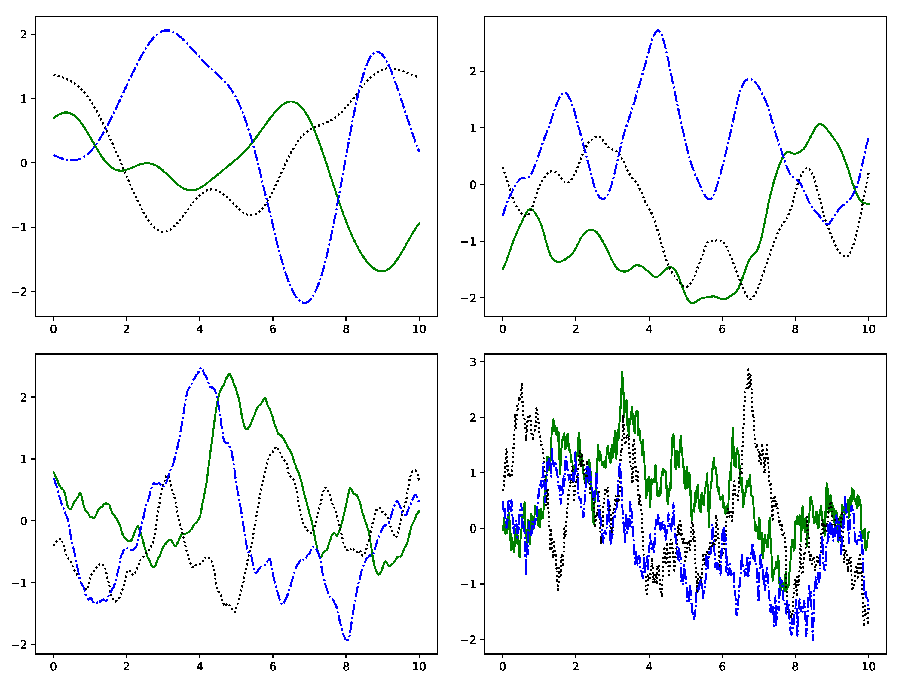
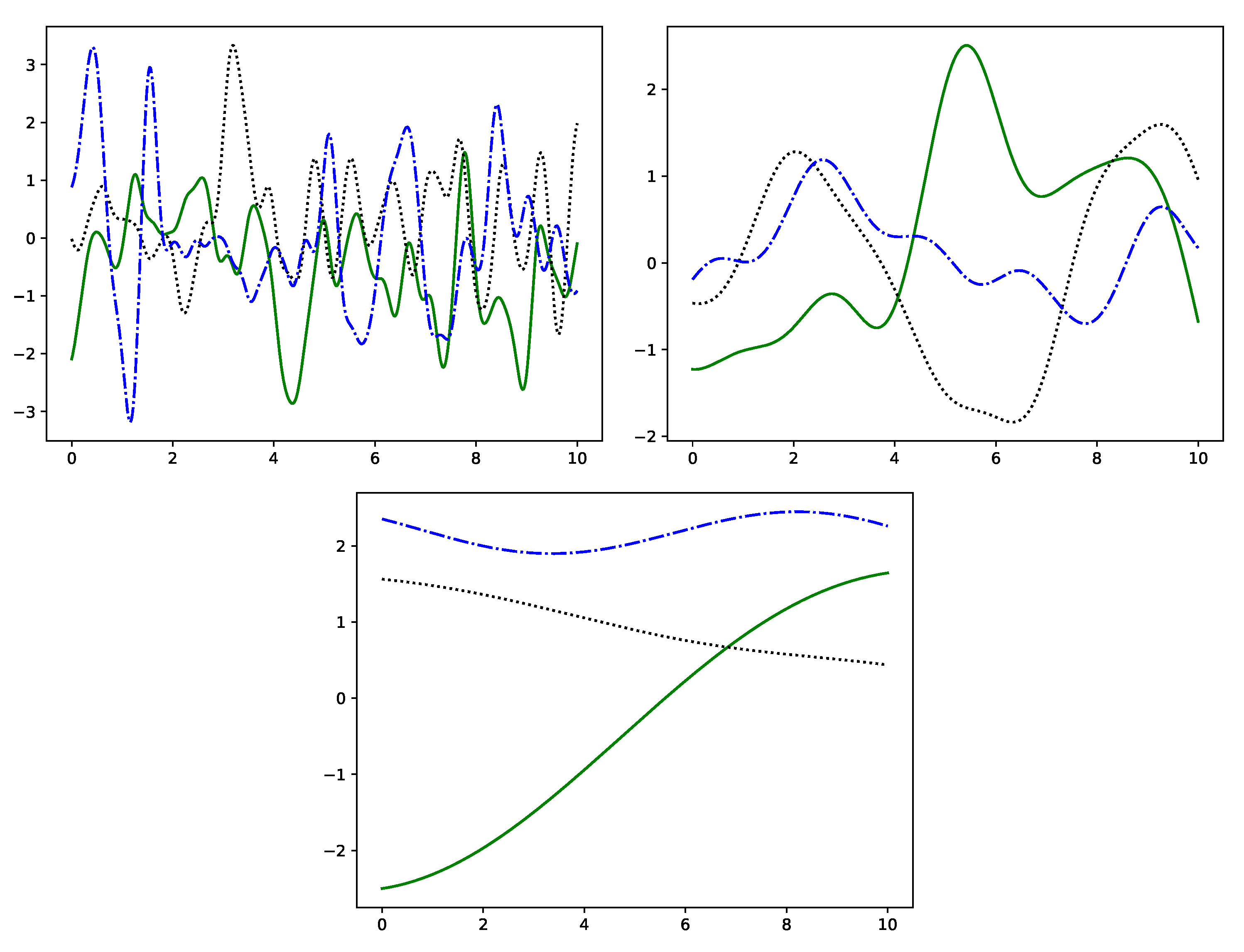
The kernels that we used for sound synthesis (see Section 3) are listed in Table 1. Figure 1 shows samples from GPs defined with different kernel functions. Many kernels have length-scale parameter ℓ, as introduced above in the formulas of the kernel functions. It controls how close two points have to be in order to be considered near and thus be highly correlated. The effect of different length-scales is illustrated in Figure 2 for a squared exponential kernel. The graphs fluctuate more rapidly with decreasing length-scale.

Table 1. The kernels from the GPy library that were used to create the wavetables.

Non-Periodic Kernels	Periodic Kernels
Exponential	StdPeriodic
ExpQuad (Exponential Quadratic)	PeriodicExponential
Matern32 ($\nu =3/2$)	PeriodicMatern32
Matern52 ($\nu =5/2$)	PeriodicMatern52
MLP (Multi-Layer Perceptron)	OU (Ornstein–Uhlenbeck)
Poly (Polynomial)
RatQuad (Rational Quadratic)
RBF (Radial Basis Function)
Spline

Figure 1. Samples from GPs with different kernels: squared exponential (upper left), Matérn 5/2 (upper right), Matérn 3/2 (lower left) and 1-exponential (lower right). All samples have length-scale parameter $\ell =1$.

Figure 2. Samples drawn from a squared exponential kernel GP with length-scale $\ell =0.1$ (left), 1.0 (right) and 10.0 (bottom).

There are operations that preserve the semidefiniteness of kernels. Let k, $k_1$ and $k_2$ be positive semidefinite kernels; then, the following kernels are also valid:

• $k_1(x_1,x_2)+k_2(x_1,x_2)$ [summing kernels],
• $k_1(x_1,x_2)k_2(x_1,x_2)$ [multiplying kernels],
• $p(k(x_1,x_2))$, where $p(x)$ is a polynomial,
• $f(x_1)k(x_1,x_2)f(x_2)$, for all functions $f:S\to \mathbb{R}$.

In GP sound synthesis, such combinations of kernels are used.

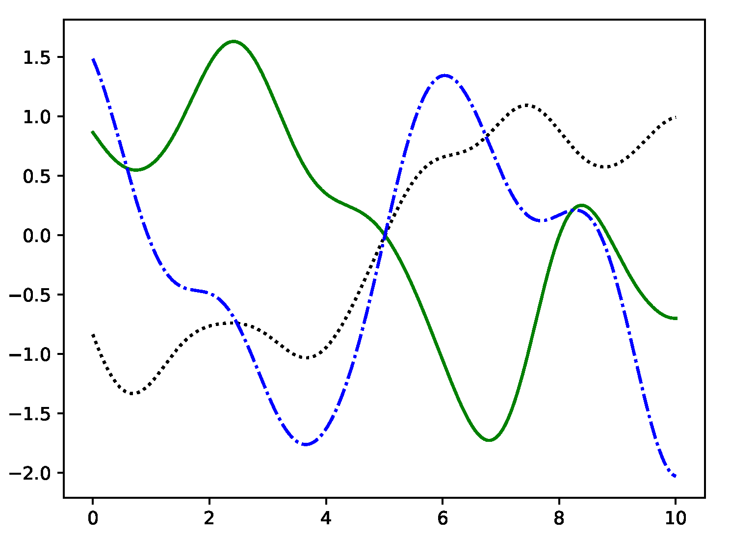
GP regression [12] (ch. 2) can be thought of as computing a posterior distribution of functions that pass through the observations (function-space view). The graphs in Figure 1 and Figure 2 were drawn from the prior distribution. With GP regression, it is possible to specify a posterior distribution with functions that pass through the observations (see Figure 3). Furthermore, it is possible to specify the uncertainty of an observation. By setting the uncertainty to zero, all samples from the posterior distribution pass exactly through the specified point (see Figure 3). We use this later to generate suitable wavetables (see Section 3.1). Computationally, GP regression is dominated by the inversion of the covariance matrix [12] (ch. 2). This has a computational complexity of $O(n^3)$, where n is the total number of points (observations + points to be sampled).

Figure 3. Five samples drawn from the posterior, conditioned on a noise-free observation at x = 5, y = 0 (squared exponential kernel, length-scale $\ell =1$). Note that all samples pass through that point.

3. GP Sound Synthesis

In GP sound synthesis, random continuous functions are sampled from a GP. These functions are then used for wavetable or waveshaping synthesis. Both wavetable and waveshaping syntheses produce sounds with harmonic spectra, where the energy is contained in integer multiples of the fundamental frequency. By sampling multiple functions from the same GP, we get individual sounds that are perceptually similar but not identical. To make sure that the generated wavetables are usable for synthesis, the following properties are enforced:

• The timbre of the synthesized sound should be controllable and depend on the choice of the kernel and its parameters.
• The perceptual loudness of the synthesized sounds should be similar, i.e., independent of the choice of the kernel and its parameters.

3.1. Generating Wavetables with GPs

In wavetable synthesis [3], a single period of a sound is stored in memory. In order to synthesize the sound at a certain pitch, the wavetable is cyclically read out at the corresponding rate. Here, the wavetable is generated by sampling equidistantly from a GP in the interval $[0,2\pi ]$ at N points $\frac{p}{N}2\pi$ for $p=0\cdots N-1$. Often, but not always, there is a distinct jump between the last ($p=N-1$) and the first sample point ($p=0$). This is also visible in Figure 1, where most graphs end at a different value than they started. A wavetable with such a sudden jump produces a sound with a considerable amount of energy throughout all harmonics. By chance, a few of the graphs in Figure 1 are continuous at the boundary: i.e., the last and the first point are close. For such wavetables, the spectrum of the sound contains considerably less energy in the higher harmonics. The energy in the harmonics thus depends on the actual shape of the graph at the boundary. This is not controllable by choosing the kernel and its parameters.

To overcome this problem, GP regression is used to ensure that the graph passes through $(0,0)$ and $(2\pi ,0)$. As mentioned above, N points $p=0\cdots N-1$ are used to construct the wavetable. We add another point and use it to ensure that the graph passes through $(2\pi ,0)$. This last point is discarded in the wavetable, where only the points $p=0\cdots N-1$ are used. Figure 4 illustrates the effect of this approach.

Figure 4. Spectrograms of GP wavetable synthesis with a squared exponential kernel. The length-scale is increased 10 times. (left) Without GP regression, there is usually more energy in the higher harmonics at smaller length-scales. If, by chance, the wavetable is continuous at its boundary, then there is a distinct change in the spectrum with a reduction of energy at the higher harmonics (marked with an arrow). (right) With GP regression, the energy in the harmonics decreases more predictably with increasing length-scale.

Another way to address the continuity at the boundary is to use periodic kernels. An example is the standard periodic kernel [13]

$$k(x_1,x_2)={\theta }_{1}exp\left[-\frac{1}{2}{\left(\frac{sin(\frac{\pi }{\lambda }(x_1-x_2))}{l}\right)}^2\right]$$

with periodicity parameter $\lambda$ and length-scale parameter ℓ. By choosing $\lambda$ appropriately, it is ensured that the generated graph has a period of $2\pi$ so that the wavetable is continuous at the boundary as required. In this case, it is not necessary to resort to GP regression. Other options are the periodic kernels of the Matérn class [14].

Ultimately, we used the kernels listed in Table 1 for sound synthesis. The spectrum of the sound generated with the aforementioned wavetables shows variation. Some kernels generate smoother functions than others: compare, for example, the curves generated from the squared exponential kernel (a kernel that is differentiable infinitely many times) with the ones created with the 1-exponential in Figure 1. The spectrum differs accordingly, with markedly more energy in the higher frequencies for the wavetables created with the 1-exponential as long as the length-scales are similar. As the length-scale controls how rapidly the graph fluctuates, lower length-scales produce wavetables with higher spectral content (see also Figure 4, right). As described in Section 2, new kernels can be created from existing kernels, for example, by adding or multiplying two existing kernels. This adds further variety to the generated sounds.

It is a well-known fact from psychoacoustics that the human perception of loudness depends on the spectral content of the sound [15] (ch. 8). Therefore, the loudness was calculated according to db(B) weighting for a synthesized middle C note. The sound was then normalized to a fixed reference loudness. After normalizing, it can occur that some sample points in the wavetable exceed the admissible range of between −1.0 and +1.0. Consider, for example, a wavetable that is close to zero most of the time and has one distinct peak that exceeds +1. This cannot be completely ruled out because of the random nature of sampling from a GP. If this happens, the wavetable is discarded and sampled from the GP again.

Overall, GP wavetable synthesis can be summarized as follows:

• Sample the wavetable from GP. Ensure that the wavetable is continuous at the boundary either (a) by using a periodic kernel or (b) by using GP regression to enforce continuity.
• Zero-center the wavetable.
• Normalize the loudness of the wavetable according to db(B)
• If a sample in the wavetable exceeds the range [−1, +1], then repeat from step 1.
• Use the wavetable for classical wavetable synthesis.

3.2. Generating Shaping Functions with GPs

In waveshaping synthesis, the signal of an oscillator is transformed by the shaping function. The shaping function maps from [−1, +1] to [−1, +1], which corresponds to the full range of audio signals. If the shaping function is nonlinear, then the timbre of the sound is changed. The output is $y=f(a(t)x(t))$, where f is the shaping function, $a(t)$ is the time-varying amplitude, usually from an envelope, and $x(t)$ is the input signal, typically an oscillator with fixed amplitude. Shaping functions can be hand-drawn or defined mathematically, e.g., with Chebyshev polynomials [5]. We used the kernel functions from Table 1 to generate shaping functions. Again, existing kernels can be combined, for example, by adding or multiplying them, to create new kernels and increase sound variety.

A shaping function is generated by sampling from the prior distribution of a GP. In contrast to wavetables, there is no wrap-around, so it is not necessary to use GP regression to enforce continuity at the boundary. The perceptual qualities of the sound depend on the chosen kernel and its parameters. To normalize the loudness across different shaping functions, we synthesize the sound on the basis of a full-scale cosine oscillator at 261.6 Hz (middle C). The loudness of the resulting sound is computed according to db(B) weighting normalized with respect to a reference. This ensures that the perceptual loudness of sounds generated with different shaping functions is similar.

3.3. Computational Aspects

Computing the Cholesky decomposition is the most expensive operation when sampling from a GP (see Section 2). It has a computational complexity of $O(N^3)$, where N is the number of sampled points. In GP sound synthesis, N corresponds to the size of the wavetable or the size of the table representing the shaping function. Balancing between computation time and sound quality, we chose $N=2205$. The other operations are considerably cheaper (see Section 2). Overall, it takes 0.54 s to compute a wavetable or a shaping function, starting from constructing the covariance matrix. When sampling multiple times from the same kernel with the same parameters, it is possible to compute the Cholesky decomposition only once and reuse it. Then, it takes only 0.041 s to compute a wavetable or a shaping function, a more than 10-fold increase in speed. In our experiments, we used this strategy to sample multiple times from the same GP more efficiently. The time measurements were done using a single core of a PC with an i7-7700K CPU running at 4.2GHz. The results were averaged over 1000 runs.

4. Sound Selection Interface

As described in the previous section, there are many different kernels that can be used to generate wavetables and shaping functions. With the length-scale, these kernels have at least one continuous parameter. Discretizing the length-scale yields #kernels × #length-scales relevant settings. If the kernels are composed, for example, by summing or multiplying, even more combinations arise. The number of combinations is so large that it is impractical for the user to enumerate all of them. Therefore, a sound navigation interface helps the user to find interesting sounds (see Figure 5). Each dot represents a short sound sample, which is played when the user clicks on the dot. The two-dimensional layout of the dots is computed by calculating a 2-D t-SNE [11] representation based on the MFCC features of the sounds. This ensures that dots in close proximity sound similar. The interface can be found here: http://www.cemfi.de/gaussian-process-synthesis, see also the Supplementary Video S1.

Figure 5. User interface for GP synthesis sound selection. When the user clicks one of the dots, the dot is marked red, and the corresponding sound is played. In the upper-left corner, the parameters of the sound are shown. In this case, the function is drawn from a GP where the kernel is the sum of a polynomial ($\ell =0.15$) and a Matérn 3/2 kernel ($\ell =0.31)$. The function is used for waveshaping.

In the interface, t-SNE is used to compute a two-dimensional embedding of the 20-dimensional MFCC feature space. t-SNE [11] uses optimization to place the data points in the low-dimensional space. From their position, t-SNE determines the similarity between points. However, similarity is defined differently in the high- and low-dimensional spaces. Similarity is based on a Gaussian distribution in the high-dimensional space and on a Student t-distribution in the low-dimensional space. This allows the optimizer to place dissimilar points far apart in the low-dimensional space. In our case, similar sounds (as judged by the distance of their MFCC vectors) are placed close to each other, while dissimilar sounds are placed far apart. Other than that, one should be careful when interpreting t-SNE-based visualizations: Wattenberg et al. [16] pointed out that t-SNE visualizations can look different depending on hyperparameter settings, that cluster sizes can be misleading and that it can be misleading to compare distances of points that are relatively far apart. Therefore, it is difficult to analyze the actual shape of the landscape in Figure 5. However, similar sounds are placed close to each other, and the user can thus efficiently explore the sound space.

The kernels listed in Table 1 are all used in the interface. The length-scale parameter ℓ is varied from 0.01 to $\pi$ in 20 equally spaced points on a logarithmic scale. For wavetable and waveshaping synthesis, the tables are computed as follows: For each setting of kernel and length-scale, seven tables are sampled. In total, this gives us 1960 different combinations (14 kernels × 20 length-scales × 7 tables). Furthermore, multiplicative and additive combinations of the kernels are used. To reduce storage, we did not enumerate all combinations of kernels, length-scales and operations (“plus“, “times“) but rather used 500 random combinations. Again, seven tables for each of those combinations were sampled in order to have seven similar but non-identical sounds per combination. To produce sounds for the sound selection interface, the waveshaping synthesis is driven with a full-scale sine oscillator.

Once the wavetables and shaping functions have been generated and stored as audio files, they are usable within any programming environment. To enable such use cases, we developed an application that encapsulates the navigation user interface (Figure 5) and sends an Open Sound Control (OSC) message when the user clicks on one of the dots. Once the OSC message is received in the programming environment (e.g., SuperCollider, pureData or Max/MSP), the corresponding audio file that contains the precomputed wavetable or shaping function is loaded by the user’s program. Audio synthesis can then be performed with the means of the programming environment. A video demonstrating the real-time interaction with the application for fixed MIDI playback can be found here: http://www.cemfi.de/gaussian-process-synthesis. Of course, live input, e.g., from a MIDI keyboard or from another controller, is also possible.

5. Related Work

5.1. GPs in Sound Synthesis and Audio Analysis

GPs have been used to synthesize natural sounds, to reproduce acoustic instrument sound, to synthesize speech and to analyze audio and music signals. Wilkinson et al. [17] used Latent Force Models to learn modal synthesis parameters. Modal synthesis is a physically inspired synthesis method [18] (ch. 4). Latent Force Models [19] combine GPs with physical models. The latent state is sampled from a GP. The observations depend on the latent state via a mechanistic model that is expressed through differential equations. An example is forces acting on springs: the forces over time are sampled from a GP, the observations are the spring positions over time, and the physical model is a second-order differential equation. Latent Force Models can be applied in various areas, including biology, motion capture and geostatistics. In the model by Wilkinson et al. [17], the system learns the stiffness and the damping constants of a mass-spring system for each mode. The modes are peak-picked from a spectrogram. The mass-spring system is modeled with a differential equation. It relates an unknown excitation function, which is sampled from a GP, to the measured amplitude over time of the mode and the mode-specific stiffness and damping constants. Wilkinson et al. used this to model and synthesize clarinet and oboe sounds (sound examples: http://c4dm.eecs.qmul.ac.uk/audioengineering/latent-force-synthesis). It is possible to interpolate the parameters and morph between two sounds. Further interaction possibilities are provided: the excitation curves can be hand-drawn [17], or the user can control the mean function of the posterior with real-time MIDI messages [20]. A further Latent Force Model by Wilkinson et al. [21] uses a difference equation that models temporal correlation by incorporating values from previous time steps. The temporal contribution is modulated by feedback coefficients (for the influence of previous output) and lag coefficients (for the influence of previous input). In combination with damping coefficients for exponential decay, amplitude envelopes are predicted for multiple frequency bands. The system was trained to re-synthesize natural sounds.

GPs have also been used to synthesize speech. For example, Koriyama and Kobayashi [22] used GP regression to predict frame-wise the acoustic features for parametric speech synthesis. The similarity of linguistic and position features is modeled in the covariance matrix. The model predicts duration, fundamental frequency, mel-cepstrum, band aperiodicity, and whether the sound is voiced or unvoiced.

GPs have been used for music information retrieval. Alvarado and Stowell used GPs to perform pitch estimation and to impute short gaps of missing audio data [23]. They modeled the musical signal by an additive superposition of periodic kernels, which are localized in time with “change windows“. For these change windows, they made use of the fact that for a given kernel k and any function $\varphi$, the expression $\varphi (x_1)k(x_1,x_2)\varphi (x_2)$ is again a kernel. In another study, Alvarado et al. used GPs for source separation in the time-domain. [24]. They modeled the different spectral characteristics of signals with spectral mixture kernels. It is also possible to extract high-level information from audio signals with GPs. Markov and Matsui [25] applied GP regression to music emotion recognition to predict valence and arousal from standard audio features such as MFCC. With the same features, GP classification predicts the genre of the music.

Analytic and synthetic approaches can be combined elegantly in the Bayesian framework. Turner [26] used GPs to develop Bayesian methods for statistical audio analysis. For this purpose, generative probabilistic models of sounds are formulated. Bayesian inference is then used on the generative models to analyze natural sounds and auditory scenes. With this approach, Turner developed Bayesian methods for probabilistic amplitude demodulation and methods for calculating probabilistic time–frequency representations. These methods are used to analyze and synthesize natural sounds and auditory scenes (sound examples: http://www.gatsby.ucl.ac.uk/turner/Sounds/sounds.html).

Cádiz and Ramos [27] used quantum physical equations to generate sound. In their work, they explored an implementation based on multiple wavetables but settled to use an approach based on additive synthesis because of its better performance.

Previous works have used GPs in the context of modal synthesis or for analysis and synthesis of natural sound. In GP synthesis, as proposed in this paper, tables are drawn from the prior distribution of a GP specified by its kernel and the kernel’s parameters. The tables are then used for wavetable or waveshaping synthesis. This is a novel way to use GPs for sound synthesis.

5.2. Interfaces for Multidimensional Sound Control

In corpus-based concatenative synthesis [28], short sound segments are chosen from a database of sounds. These segments are then assembled to produce the resulting sound. A target sound can be re-synthesized from the sound segments. To re-synthesize a sound, a selection algorithm matches descriptors of the sound segments with the descriptors of the target sounds. Furthermore, the cataRT interface allows a user to interactively navigate the sound space of the corpus by arranging the sounds in two dimensions by mapping the values of the descriptors to the x- and y-coordinates.

Grill and Flexer developed an interface where auditory–visual associations are used to organize textural sounds visually in an intuitive manner [29]. Auditory properties, such as “high-low”, “ordered-chaotic” and “tonal-noisy”, are mapped to perceptually corresponding visual features. For example, “high-low” is mapped to a combination of color and brightness (from bright yellow to dark red). However, the auditory properties are not automatically detected. They come from a manually annotated dataset. Later, Grill [30] developed computable audio descriptors for these perceptual features in order to use the system without manual tagging.

Pampalk et al. [31] mapped songs of a large music collection to a two-dimensional map such that similar pieces are located close to each other. To compute the mapping, they developed a special processing pipeline to compute features representing sound similarity. The songs are mapped to the two-dimensional plane by applying Self-Organizing Maps (SOM) on the sound similarity features. A SOM is a neural network trained in a supervised manner to learn a low-dimensional representation of the input data. Pampalk et al. also applied their approach to the visualization of drum sample libraries [32].

Similarly, Heisen et al., used MFCC and SOM to visualize large audio collections [33]. Their SoundTorch provides an interface where the user controls a virtual light cone that shines on the mapped points of the source sounds. These sounds are played back simultaneously with sound spatialization.

Even after filtering a query with tags, hundreds of potential candidate sounds often remain. Frison et al. [34] used t-SNE based on MFCC features to calculate a similarity-based point cloud map of sounds. The visual layout is aimed to help sound designers to choose a sound. Furthermore, they mapped audio features (YAAFE: perceptual sharpness) to the color of the points. Frison et al. developed and evaluated a variety of interfaces where sounds are mapped to 2D locations. The users perform a known-item search task. Setagro et al. used t-SNE on a variety of audio features to analyze the timbre of historical and modern violins [35].

Our sound selection interface is similar to existing interfaces for sound navigation. Like the system by Frison et al. [34], our interface uses a t-SNE embedding based on MFCC features to visualize sound similarity in two dimensions.

6. Conclusions

In GP sound synthesis, functions are sampled randomly from GPs. The random functions are then used as tables in wavetable synthesis or as shaping functions in waveshaping synthesis. The shape of the function can be controlled by choosing a kernel function and its parameters. Most kernel functions have at least one parameter: the length-scale ℓ. It controls how fast the correlation between two points decreases with distance. With lower length-scale, the randomly sampled function oscillates faster, which leads to a spectrum with more high-frequency energy. Furthermore, kernel functions can be combined in multiple ways. We explored additive and multiplicative combinations, but there are more possibilities to be explored in the future, including Deep GPs. Even now, the number of choices (kernels, their parameter(s) and their additive and multiplicative combinations) makes it impractical for a user to explore the possible sounds by enumerating everything. A user interface based on a visual map, where the sounds are grouped according to their similarity, aids the user in sound selection.

References

1. Holmes, T. Electronic and Experimental Music: Technology, Music, and Culture; Routledge: London, UK, 2012. [Google Scholar]
2. Davies, H.S. The New Grove Dictionary of Music and Musicians; Sadie, S., Tyrrell, J., Eds.; Grove: New York, NY, USA, 2001; p. 219. [Google Scholar]
3. Bristow-Johnson, R. Wavetable synthesis 101, a fundamental perspective. In Audio Engineering Society Convention 101; Audio Engineering Society: New York, NY, USA, 1996; pp. 1–27. [Google Scholar]
4. Chowning, J.M. The synthesis of complex audio spectra by means of frequency modulation. J. Audio Eng. Soc. 1973, 21, 526–534. [Google Scholar]
5. Roads, C. A tutorial on non-linear distortion or waveshaping synthesis. Comput. Music J. 1979, 3, 29–34. [Google Scholar] [CrossRef]
6. Smith, J.O. Physical Audio Signal Processing: For Virtual Musical Instruments and Audio Effects; W3K Publishing: Stanford, CA, USA, 2010. [Google Scholar]
7. Roche, F.; Hueber, T.; Limier, S.; Girin, L. Autoencoders for music sound synthesis: A comparison of linear, shallow, deep and variational models. arXiv 2018, arXiv:1806.04096. [Google Scholar]
8. Engel, J.; Resnick, C.; Roberts, A.; Dieleman, S.; Norouzi, M.; Eck, D.; Simonyan, K. Neural audio synthesis of musical notes with wavenet autoencoders. In Proceedings of the 34th International Conference on Machine Learning-Volume 70, Sydney, NSW, Australia, 6–11 August 2017; pp. 1068–1077. [Google Scholar]
9. Donahue, C.; McAuley, J.; Puckette, M. Adversarial audio synthesis. arXiv 2018, arXiv:1802.04208. [Google Scholar]
10. Kiefer, C. Sample-level sound synthesis with recurrent neural networks and conceptors. PeerJ Comput. Sci. 2019, 5, e205. [Google Scholar] [CrossRef]
11. Maaten, L.v.d.; Hinton, G. Visualizing data using t-SNE. J. Mach. Learn. Res. 2008, 9, 2579–2605. [Google Scholar]
12. Rasmussen, C.E. Gaussian processes in machine learning. In Summer School on Machine Learning; Springer: Amsterdam, The Netherlands, 2003; pp. 63–71. [Google Scholar]
13. MacKay, D.J. Introduction to Gaussian processes. NATO ASI Ser. F Comput. Syst. Sci. 1998, 168, 133–166. [Google Scholar]
14. Durrande, N.; Hensman, J.; Rattray, M.; Lawrence, N.D. Gaussian process models for periodicity detection. arXiv 2013, arXiv:1303.7090. [Google Scholar]
15. Zwicker, E.; Fastl, H. Psychoacoustics: Facts and Models; Springer Science & Business Media: Berlin/Heidelberg, Germany, 2013; Volume 22. [Google Scholar]
16. Wattenberg, M.; Viégas, F.; Johnson, I. How to use t-SNE effectively. Distill 2016, 1, e2. [Google Scholar] [CrossRef]
17. Wilkinson, W.J.; Reiss, J.D.; Stowell, D. Latent force models for sound: Learning modal synthesis parameters and excitation functions from audio recordings. In Proceedings of the 20th International Conference on Digital Audio Effects, Edinburgh, UK, 5–9 September 2017; pp. 56–63. [Google Scholar]
18. Cook, P.R. Real Sound Synthesis for Interactive Applications; AK Peters/CRC Press: Boca Raton, FL, USA, 2002. [Google Scholar]
19. Alvarez, M.; Luengo, D.; Lawrence, N.D. Latent force models. In Proceedings of the 12th International Conference on Artificial Intelligence and Statistics, Clearwater Beach, FL, USA, 16–18 April 2009; pp. 9–16. [Google Scholar]
20. Wilkinson, W.; Stowell, D.; Reiss, J.D. Performable spectral synthesis via low-dimensional modelling and control mapping. In DMRN+11: Digital Music Research Network: One-Day Workshop; Centre for Digital Music, Queen Mary University of London: London, UK, 2016. [Google Scholar]
21. Wilkinson, W.J.; Reiss, J.D.; Stowell, D. A generative model for natural sounds based on latent force modelling. In International Conference on Latent Variable Analysis and Signal Separation; Springer: Cham, Switzerland, 2018; pp. 259–269. [Google Scholar]
22. Koriyama, T.; Kobayashi, T. A comparison of speech synthesis systems based on GPR, HMM, and DNN with a small amount of training data. In Proceedings of the 16th Annual Conference of the International Speech Communication Association, Dresden, Germany, 6–10 December 2015; pp. 3496–3500. [Google Scholar]
23. Alvarado, P.A.; Stowell, D. Gaussian processes for music audio modelling and content analysis. In Proceedings of the 2016 IEEE 26th International Workshop on Machine Learning for Signal Processing (MLSP), Salerno, Italy, 13–16 September 2016; pp. 1–6. [Google Scholar]
24. Alvarado, P.A.; Alvarez, M.A.; Stowell, D. Sparse gaussian process audio source separation using spectrum priors in the time-domain. In Proceedings of the ICASSP 2019 IEEE International Conference on Acoustics, Speech and Signal Processing (ICASSP), Brighton, UK, 12–17 May 2019; pp. 995–999. [Google Scholar]
25. Markov, K.; Matsui, T. Music genre and emotion recognition using Gaussian processes. IEEE Access 2014, 2, 688–697. [Google Scholar] [CrossRef]
26. Turner, R.E. Statistical Models for Natural Sounds. Ph.D. Thesis, UCL (University College London), London, UK, 2010. [Google Scholar]
27. Cádiz, R.F.; Ramos, J. Sound synthesis of a Gaussian quantum particle in an infinite square well. Comput. Music J. 2014, 38, 53–67. [Google Scholar] [CrossRef]
28. Schwarz, D. Corpus-based concatenative synthesis. IEEE Signal Proc. Mag. 2007, 24, 92–104. [Google Scholar] [CrossRef]
29. Grill, T.; Flexer, A. Visualization of perceptual qualities in textural sounds. In International Computer Music Conference; International Computer Music Association: San Francisco, CA, USA, 2012; pp. 589–596. [Google Scholar]
30. Grill, T. Constructing high-level perceptual audio descriptors for textural sounds. In Proceedings of the 9th Sound and Music Computing Conference, Copenhagen, Denmark, 12–14 July 2012; pp. 486–493. [Google Scholar]
31. Pampalk, E.; Rauber, A.; Merkl, D. Content-based organization and visualization of music archives. In Proceedings of the 10th ACM International Conference on Multimedia, Pins, France, 1–6 December 2002; pp. 570–579. [Google Scholar]
32. Pampalk, E.; Hlavac, P.; Herrera, P. Hierarchical organization and visualization of drum sample libraries. In Proceedings of the 7th International Conference on Digital Audio Effects (DAFx’04), Naples, Italy, 5–8 October 2004; pp. 378–383. [Google Scholar]
33. Heise, S.; Hlatky, M.; Loviscach, J. Soundtorch: Quick browsing in large audio collections. In Audio Engineering Society Convention 125; Audio Engineering Society: New York, NY, USA, 2008. [Google Scholar]
34. Frisson, C.; Dupont, S.; Yvart, W.; Riche, N.; Siebert, X.; Dutoit, T. Audiometro: Directing search for sound designers through content-based cues. In Proceedings of the 9th Audio Mostly: A Conference on Interaction With Sound; ACM: New York, NY, USA, 2014; pp. 1–8. [Google Scholar]
35. Setragno, F.; Zanoni, M.; Sarti, A.; Antonacci, F. Feature-based characterization of violin timbre. In Proceedings of the IEEE 2017 25th European Signal Processing Conference (EUSIPCO), Kos Island, Greece, 28 August–2 September 2017; pp. 1853–1857. [Google Scholar]
Article Metrics
Citations
Article Access Statistics
Multiple requests from the same IP address are counted as one view.