Abstract
This paper proposes a new method of image decomposition with a filtering capability. The image state ensemble decomposition (ISED) method has generative capabilities that work by removing a discrete ensemble of quanta from an image to provide a range of filters and images for a single red, green, and blue (RGB) input image. This method provides an image enhancement because ISED is a spatial domain filter that transforms or eliminates image regions that may have detrimental effects, such as noise, glare, and image artifacts, and it also improves the aesthetics of the image. ISED was used to generate 126 images from two tagged image file (TIF) images of M87 taken by the Spitzer Space Telescope. Analysis of the images used various full and no-reference quality metrics as well as histograms and color clouds. In most instances, the no-reference quality metrics of the generated images were shown to be superior to those of the two original images. Select ISED images yielded previously unknown galactic structures, reduced glare, and enhanced contrast, with good overall performance.
1. Introduction
There is need to provide a highly tunable fundamental image processing technique that can remove unwanted color, biased glare, and noise; reduce image artifacts; and improve the contrast and aesthetics in a post-processed RGB image. Generally, one has two main paths to follow when applying image decomposition or enhancement. One typically chooses to be in either the spatial domain or the frequency domain. The image state ensemble decomposition method (ISED) uses sets of spatial domain filters that decompose an image by selectively removing discrete state ensembles from the original image in a red, green, and blue (RGB) color space. This removed portion of the image contains a range of color information that encompasses regions of the image with noise that may biased to a certain domain of the image. These regions may also contain unwanted artifacts and glare. ISED generates images to help discover these biased regions and reduces the unwanted characteristics from the image. ISED generates possible image outcomes from the information contained within a post-processed RGB image. Additionally, ISED is a novel approach that is applicable in many fields; astronomical imaging was chosen out of personal interest.
In the spatial domain, direct manipulation of the pixels is normally modified by averaging, median filtering, contrast stretching, Gaussian blurring, many types of histogram equalizations (HE), and the Retinex algorithm, just to name a few [1,2,3,4]. These methods suffer from major drawbacks where the pixel information is either blurred, redistributed, or the intensity is scaled in an unrealistic way [1,3]. ISED is an image decomposition method that has the ability to remove unwanted color and biased glare, reduce noise, improve contrast, reduce image artifacts, and improve the aesthetics in a post-processed RGB image. ISED retains all of the photonic information from the original information if one simply recombines the ISED image and the ISED filter; provided that the image is saved in a lossless format such as tagged image file (TIF) or PNG, one would have the original image with a structural similarity index (SSIM) equal to 1. Therefore, the process is fully reversible, and the information can be conserved. This is unlike the aforementioned conventional image processing methods, which in essence have a loss or distortion of pixel information. However, the standard image processing techniques are very useful in a case-by-case basis, such as using the median filter to clean salt and pepper noise, using an averaging filter to reduce random statistical noise, and using some form of histogram equalizations (HE) or Retinex to redistribute pixel information to enhance contrast [1,2]. With ISED, you can be more selective about the informative structures that you wish to study and can extract features in a way that does not corrupt the information in the image. It creates classes of possible filters and possible images, while preserving information, which is dissimilar to existing methods. ISED provides details of structures previously not seen in the images processed by NASA (The National Aeronautics and Space Administration), JPL-Caltech (Jet Propulsion Laboratory, California Institute of Technology), and IPAC (Infrared Processing and Analysis Center).
ISED is able to maintain the information of the selected image and move portions of the image to the filter. Thus, there is no loss of pixel information if both the image and filter are known. Therefore, there is no loss of entropy when the ISED filter is recombined with the filtered ISED image: you obtain the original image. With ISED, one can simply generate many possible images from the original image, and as a result of this study, ISED has the ability to show features of galactic structures that were previously hidden within the initial image. Therefore, the need and the purpose of the specific example studied in this paper is to reveal new visual information about M87′s galactic structure. The ISED method is not limited to astronomical applications but can be applied to any color image or video. This novel method is akin to Schrödinger’s cat [5,6] but with a deterministic twist. There is a cat in a closed box, but with ISED, I can simply change the color of the cat, decide if the cat has no hair, or make part of the cat invisible. Maybe at a certain instance in time the cat is purring, sitting, or sleeping. The cat can move around freely and be relatively comfortable inside its box. We know the cat is inside, but we do not know its current state until we decide to peek inside the box. An image is similar to Schrödinger’s cat in that the light collected from an image is a record of various flavors of photons that are counted, stored, and allocated to a specific location in order to form a record of the photons. This record is the image, which I reiterate is the representation of an occurrence of photonic information observed over some time interval. Since the image is a record of photonic information, the use of statistics should be employed to remove a finite collection of photonic information from the image or in other words remove discrete quanta. Additionally, all the ISED images analyzed in this paper along with Supplementary ISED-generated images and ISED filter images can be accessed online at [7]. Currently, the Supplemental images are related to the topics of art, astronomy, general photography, histology, and mineralogy [7].
General relativity was introduced by Einstein in 1917 [8]. One result of the Einstein field equations (EFEs) was the theoretical concept of black holes. Schwarzschild noticed this bizarre effect in the EFEs [8]. From this, Schwarzschild calculated that if an immense nonrotating mass is present, an object can exist with gravitational forces so strong that even light, the fastest known object in the universe, could not escape the object’s grasp [9]. Prior to the validation of the existence of black holes, Wheeler coined the term “black hole” in a lecture [10]. This theoretical construct was later confirmed by Webster et al. [11] and Bolton [12] to be a physical reality when they observed Cygnus X-1. Black holes are fascinating, mysterious, and have captivated many scientists. In a recent study, the Event Horizon Telescope collaboration produced the first image of a black hole [13]. It was presented alongside photographs taken by the Spitzer Space Telescope (SST) as an inset [14]. These SST images were used as the input data for this study.
In order to improve the visualization of post-processed SST images and thus reveal more informative visual details and improve our understanding of the nature and structure of the universe, we propose ISED. ISED uses a series of cross-channel relations made between the red (R), green (G), and blue (B) color channels. A pixel in a modern monitor uses additive mixing color theory, wherein colors can be added and mixed from three primary colors: red, green, and blue (RGB). Additive mixing theory was introduced by Maxwell in “On the Theory of Compound Colours, and the Relations of the Colours of the Spectrum” [15]. The standard monitor operates with the pixels being a certain ratio/mix of varying intensities within the RGB color channels. This system is scaled from 0 to 255, in which 0 is black and 255 is the highest intensity in the color channel. Therefore, a standard pixel can represent 2563 different colors. These pixel intensities combine in a matrix to form an image. The cross-channel relationship in ISED is designed to be a possible set of states. The ensemble of states can either exist (as “on”) or not (as “off”) for the most basic case. These ensemble states can overlap regions of an image that contain unwanted pixel information, such as glare. If a region contains glare biased to a particular color channel, one can reduce the effects by selecting the correct ISED state. This switch choice depends on the desired image outcome and the input image. One may output various image states and simply compare the characteristics of the ISED-generated image for the desired outcome. For example, the ISED filter can remove glare that is biased to a certain bandwidth of color while maintaining the structure of the image of interest. Once the correct ISED state is determined for this particular image solution, you can apply the same state selection to a similar image to yield the desired results.
The paper is organized as follows. Section 2 provides an overview of the materials and methods used to generate ISED images. Section 3 provides the mathematical framework to construct ISED images and filters. Section 4 presents the experimental results and discussion of this study. Finally, the conclusion in Section 5 gives the ramifications of ISED.
2. Materials and Methods
In the proposed ISED experiments, MATLAB R2018a and R2019a were used to implement our proposed algorithm on the post-processed SST image sets. The images were sourced from NASA/JPL-Caltech/IPAC. The implemented hardware configuration was comprised of an Intel i7-8750H processor, 32 GB of RAM, and an NVidia GeForce GTX 1060 graphics processing unit. The experimental input data were sampled images of M87. The first file, “ssc2019-05c.tif”, is 11.2 MB in size with a pixel resolution of 3580 × 3580. The second image of M87, file name “ssc2019-05b.tif”, is 11.1 MB in size with a pixel resolution of 3580 × 3580. The inset of this second image contains an enlarged region of M87′s core, in which the region of M87′s black hole and its jets are shown. This inset was cropped by using GIMP 2.10.14 and saved as a lossless tagged image file (TIF) format for processing. The remainder of the image in file “ssc2019-05b.tif” was discarded, because “ssc2019-05c.tif” is the same image without the inset. The size of the cropped image was 1.54 MB with a pixel resolution of 730 × 733. The two images were taken by the SST using an Infrared Array Camera (IRAC). The nominal values of the red, green, and blue channels were mapped to the IRAC infrared radiation wavelengths of 8.0, 4.5, and 3.5 μm, respectively [14]. Both images were generated with chromatic ordering taken from the infrared portion of spectrum. Therefore, the images were an approximation of what we see if the sampled photons were in the visible range of the spectrum. The physical filter selection can cause part of the continuum sources (e.g., a star) to not exhibit true color, such as the case of a narrow-band filter not properly sampling the stellar blackbody [16]. The ISED filter can operate in a similar manner by reducing a narrow band of the image matrix information.
The two images were separated into their constitute components. The intensities of the individual trichromatic components of red, green, and blue shall be referred to as R’, G, and B’ respectively. The R’, G, and B intensity values range from 0 to 255. The “zero” value represents black, and as the value increases on the scale, the pixel becomes lighter [1]. To generalize the problem, assume that the three color channels of the image do not have the same corresponding color channel pixel values for a discrete range between respective R’, G, and B’ image matrices. Taking this into account, difference relationships were formulated between the color channels to modify the post-processed images. This process is implemented in the spatial domain; the ISED image is matrix-wise transformed or generated at the pixel level.
For the sake of analogy, let us say that the image is analogous to the Gibbs microcanonical ensemble wherein a statistical ensemble is used to know all the possible states of a system [17]. The photons are converted to electrons via the photoelectric effect [18], counted discretely, and then categorized into three discretized groups, or color channels, to represent a single RGB pixel. Multiple pixels combine to form an image matrix. This matrix contains the information of many possible states, as ISED will later demonstrate. ISED can transfer photonic information in varying amounts from the ISED image to the ISED filter without losing any information. The sum of the image and filter equals the input image. Use of this method is possible because quantum mechanical objects (e.g., photons) can behave as waves or particles [19,20], and waves can be observed as single quanta [21]. The proposed method decomposes images without loss, provided that the information of both the image and filter is stored.
Theorem 1.
ϕn ≡ The scalar probability of an ensemble of states to either succumb to wave collapse and be measured or to not be detected. The regions of the wave collapse are bounded the probability of [0,1].
The variable ϕn is similar to a fuzzy set unit interval [0,1] to help deal with the statistical nature of light. Theorem 1 is also analogous to the infinite square well model in quantum mechanics, where the particle is bound between 0 and L and has a probability of having a certain positive energy level somewhere inside the well and at a certain moment in time. The ϕ indices, m and n, are index notations indicating that this function is applied pixel-wise in the ψ ensemble matrices.
Mathematically for this method, this set is convenient to use to determine whether a state ensemble is activated and to what degree. This image processing method takes advantage of the particle-like behavior of light and uses elements of statistical ensembles to define subsets or portions of the image. These subsets are a discrete ranges of mixed color values. Furthermore, the ISED method does not need to be a binary decision of “on” and “off” states; however, in the most elementary of applications, binary switching yields useful results. Additionally, in the most basic case, the state ensemble exists or it does not. Then, the binary conditions of, “0” or “1,” yield up to 218 different possible states of decomposition and can hence generate 218 possible images and 218 possible filters. We now turn to formulating the state ensembles and remove some “fuzziness” from an image that contains a super massive black hole.
3. Mathematics of ψ Image State Ensembles
The following novel mathematical formulas govern the behavior of the proposed ISED method. The pixel-wise function ϕn where, n = [1,2,3,…,6].
3.1. ψ Color Channel Relations
The following equations are the color channel relations for the development of ISED.
where matrix ψ is constrained by the values, ψn ≥ 0, and n = [1,2,3,…,6]. In order to simplify the experimental amplitudes of the variables, α and β are set to 1. Variables α and β can be used to change the intensity scaling of the ensemble in the image matrix. The aforementioned ψ-state ensembles are intended for an RGB image. However, the concept can be generalized for a higher dimensionality state comparison that would allow for the further mixing of colors and more state ensembles; hence, additional ISED images can be generated.
3.2. Generalized ψ Image State Ensemble Constitutive Relationships for N-wavelength λ
The following equations are the generalized ψ image state constitutive relationships, and they can be used to formulate n-color channels.
with the constraint that matrix difference values, ψn ≥ 0, o ≠ p.
3.3. ψ Ensemble Matrices for ϕn = [0,1], αn = βn = 1
The ensemble matix relationships are designed to produce a binary decision to construct the matricies that build the ISED filters.
with the constraint that matrix difference values, ψn ≥ 0.
For Equation (3), ϕn = [0,1] indicates the on and off states for the ψ matrix state ensemble. These are the ψ1, ψ2, ψ3, ψ4, ψ5, ψ6 conditions that were applied in the following systems of equations to obtain the results in this paper.
3.4. Image State Ensemble Decomposition
Below are the ISED equations with a scaling factor included to modify the intensity of the the origional images R’, G’ and B’ color channels.
where An = 1, An is an intensity scaling factor and can be used to change the intensity of the original color channel. In this experiment, An is set to 1.
3.5. Simplified Image States Ensemble Decomposition
Beneath are the novel simplified ISED equations which can be used to genrate ISED image and ISED filters. The filter component is the difference portion of the equation.
The equations in (5) can be used to generate 218 possible filters and 218 possible images based on the above formula. The matrix variables Rn, Gn, and Bn are the resultant image color channels after the desired image states have been assigned ϕn values. The values are 0 or 1 in our bivariate case. Afterwards, the resultant image color channels are recombined to form the generated image (RGB)n.
3.6. Generalized Image States Ensemble for N-Dimensions
This generalized equation can be used to set up an ISED relation between 2 to n color channels.
3.7. Balanced Image State Ensemble Decomposition for RGB
The following equation is the summation notation for the balanced ISED states studied in this paper.
This paper demonstrates and analyzes the “balanced state” condition, which is defined by the image state ensemble relationship in Equation (7) wherein the R’, G’ and B’ ψ image states are set to “on” (1) or “off” (0). For clarification, if ψ6 is set to the “on” state for the red channel, that means it will also be set to “on” for the green and blue channels. This is called a “balanced state”. In all, there are 64 balanced states possible for this configuration; however, for the “zero” image state, all ψ are set to “off” (0). Therefore, the output image is equal to the input image, and the filter is a zero image or black.
4. Results and Discussion
Image quality assessments (IQAs) were used to evaluate the experimental results; both full-reference and no-reference quality metrics were used. The no-reference metrics are able to analyze both the test image and those of the ISED images. The full-reference metrics compare the original image to the modified image for quality assessment. Full-reference quality metrics are used with the original NASA reference image, such that the modified image is compared with the original image. The full-reference quality metrics that were used are the peak signal-to-noise ratio (PSNR), image mean squared error (IMSE), and structural similarity (SSIM) index [22]. The SSIM generates a maximum score of one based on the images comparative contrast, local structure, and luminescence [22]. The IMSE is the squared error between the original image and a compressed image, whereas the PSNR is the peak error in the image. The IMSE and PSNR are used to show the amount of compression for an image, but for the case of decomposition, it can be used to gauge the relative change between the original image and the ISED image. A table of values was output for the SSIM, IMSE, and PNSR, and the results are detailed in Appendix B. For the experiment, the no-reference quality metrics statistically compare the features of the original image to those of the modified images. Furthermore, the image results shown in this paper and on the Supplemental website clearly indicate the potential worth of this filter method. In Fact, the no-reference IQAs in some instances have improved the perceptual quality over the original NASA image and show more details. The no-reference quality metrics implemented were the perception-based image quality evaluator (PIQE) [23,24], natural image quality evaluator (NIQE) [25], and blind/reference-less image spatial quality evaluator (BRISQUE) [26,27]. PIQE analyzes the local variance to see if the image has a block-wise distortion to calculate the quality of an image; lower scores are better [23]. NIQE is trained on a database of pristine images that uses nature scene statistics, in concert with Gaussian distributions, so that it can measure arbitrary distortions in the test image [25]. BRISQUE is also trained from a database of known distortions and pristine images; this method is limited to evaluating only the types of distortions that have been trained for the database [26,27]. A table of values was output for PIQE, NIQE, and BRISQUE, as shown in Appendix C. The IQAs are discussed in the results and discussion sections. Furthermore, histograms and color clouds of the images were used to show the pixel distribution over the RGB color space.
The following pseudocode flow chart in Figure 1 illustrates the design of ISED images and filters, and Algorithm 1 is for ISED generation.
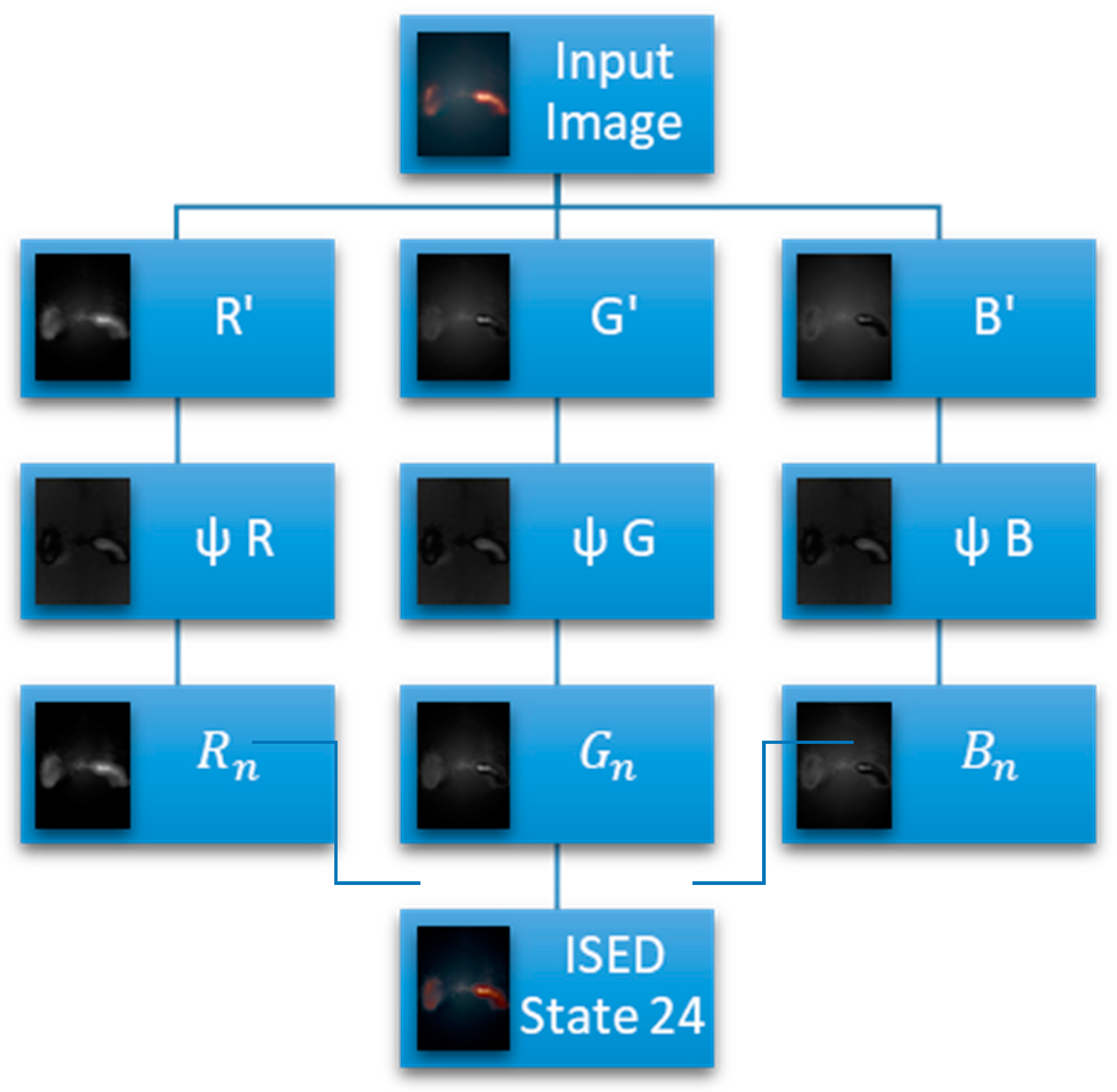
| Algorithm 1 ISED Generation |
| 1: Load the input image. |
| 2: Separate the image into its color channels R’, G’, and B’ in RGB color space. |
| 3: Use Equation (3) is used to build the filters for ψ R, ψ G, and ψ B. . |
| 4: Set the [0,1] state conditions from Appendix A, for ψ1, ψ2, ψ3, ψ4, ψ5, ψ6. This defines the state ensemble conditions. 5: The ISED color channel filter is for ψ R, ψ G, and ψ B. The combination of ψ R, ψ G, and ψ B would produce the ISED filter image. An example of an ISED filter image is shown in Figure 2c. |
| 6: Applying Equation (5) forms the modified Rn, Gn, and Bn color channels. These channels are used to build the ISED Image. |
| 7: Recombine the color channels to form a newly generated ISED image in (RGB)n. 8: Output the ISED image 9: Optional Output the ISED filter image. Original image – ISED image = ISED filter image or equivalently combine recombine the color channels from ψ R, ψ G, and ψ B to build ψ(RGB). |
Figure 1.
Algorithm flow chart for image state ensemble decomposition (ISED).
Figure 2.
Image results for a full-sized tagged image file (TIF)-format image of M87 (a) original high resolution, credited to NASA/JPL-Caltech/IPAC, (b) ISED-generated image for the sixth ensemble state condition, and (c) image of the sixth ISED filter.
According to Figure 2b, the ISED image produces well-defined regions in M87, and previously obscured structures become more pronounced. Some of the more distant galaxies have been reduced or removed; however, the larger structure is observed in greater detail with the additional advantage of reduced glare, making the detailed structure of the core of the galaxy more prominent. This unique process makes it possible to see somewhat into the interior structure of the galactic structures, similar to how an X-ray can see the bones in the human body. There appears to be a great deal of information that can be learned for the chromatic ordered images by using ISED: much more detail than the original image (Figure 2a), the ISED image (Figure 2b) has SSIM (0.79), IMSE (128.8), PSNR (26 dB), NIQE (5.32), PIQE (58.1), and BRISQUE (44.1) values. See Appendix B and Appendix C.
The states in Table 1 correspond to Equation (5), where the simplified state ensemble of the ISED image generated (in Figure 2b) is produced from Equation (7).
Table 1.
Balanced state ensemble of the sixth ISED generated image (seen in Figure 2b). RGB: red, green, and blue.
Finally, the ISED image is made after the three color channels Rn, Gn, and Bn are combined to form the image (RGB)n.
In Figure 3b, the branch on the left side of the color cloud has been removed, and Figure 3c presents the information remaining from the original image: the ISED filter.
The third histogram is state 6 ψ and that of the ISED filter. A standard horizontal axis of a histogram ranges from 0 to 255; however, in this instance, nothing substantial occurs in the image for the intensity value above 100, and the scales for the histograms have been adjusted accordingly. The image is rather dark, so most of the information and interesting features are under 80 for the RGB value displayed in Figure 4. With this filter, some information is shifted to increase the dark pixel count, yet it maintains a majority of the SSIM (0.79). Appendix B indicates that the other IQAs are on par with or superior to the original in regards to the no-reference quality metrics.
Figure 4.
Individual histograms of red (R), green (G), and blue (B) components of the (a) original image, (b) ISED image of state 6, and (c) the ISED filter image of state 6.
In Figure 5b, the structure of the jets that were expelled from the black hole in the center of M87 improved. The galactic core with its supermassive black hole is also markedly pronounced, because the biased blue glares in the background of Figure 5c were partially removed by the ISED filter. The remaining structure of the region of interest was maintained, with improved contrast enhancement over the low deterioration SSIM. The bright knots of HST-1 and a second knot are much more apparent. Additionally, the flare ejected from the supermassive black hole is more prominent. Similarly, the jets are visible in greater detail, and the core is also more pronounced and its boundary is well defined when compared to the original image. Furthermore, the ISED-generated image is also less blurred than that of the original. In Figure 5d, SSIM is higher than in the image in Figure 5c. This is useful in certain instances to be discussed in more detail in a follow-up paper. Most of the ISED generated images in this study provide the clearest view and most of the detail of M87s core, knots, and its jets currently in publication. Note that the results seen in Figure 5 do not reflect necessarily the best perceptual quality results, but rather only a sample. Additionally, the majority of the generated images have better no reference IQAs than those of the original image. So, this method is useful for analysis, and the images look beautiful. The full set of released generated images can be seen online at [7].
Figure 5.
Cropped images of (a) original image, credited to NASA/IPL-Caltech/IPAC, (b) 22nd ISED-generated image, (c) 23rd ISED-generated image, and (d) the 24th ISED-generated image.
Table 2.
Balanced state ensembles of ISED generated images in Figure 5a–c.
The experimental results are presented in Figure 6b–d. The red-portioned point clouds are shifted down and observed as a reduction of jet saturation in the ISED-generated images. The intensities of the images in Figure 5b,c have remarkably diminished, but the informative structural features of the core, jets, and knots are maintained.
In Figure 7b, the recognizable values exhibit a left-shifting of the red component to approach “zero” value (i.e., black), reducing the “reddishness” (R) of the image. Both the green and blue pixel counts are shifted as well, reducing the oversaturation of the bright jets in the original image and making them appear clearer. Furthermore, the structural detail is visually enhanced by the contrast improvement. The histogram in Figure 7c indicates that the blue and green values are less shifted than in Figure 7b, allowing for greater contrast and structural detail. The histogram in Figure 7d reveals that all the red, blue, and green pixel counts are shifted closer to the “zero” value, which is known as the “black” state. This produces a darker image, one that has the highest SSIM among the three ISED-generated images, in Figure 5b–d.
This zoomed-in cropped image is taken to show greater details of the galactic core in M87. Figure 8b shows that the structural details of the galactic core are improved and glare blurring is reduced. The core and the knots are much more apparent. In Figure 8c, the details of the galactic core have the most improvement, and the contrast is enhanced. One can easily see that the core and the knots have the greatest detail. This image also exhibits further reduction in the strong blue biased glaring that is seen in the original image. For Figure 8d, the details are slightly deteriorated over a somewhat darker background. It has a reduction in some of the reds, which have shifted to the darker values shown in Figure 8d.
The results indicate that ISED makes it possible to remove select quanta from a stellar image, and other informative features such as the core, knots, and jets became more pronounced. Figure 9 is a collage of 63 ISED-generated images and most images reveals details that were previously obscured. This method has tremendous potential to peer into the heart of a galaxy. Structures of the galaxy, seen in Figure 2, lose some of their “fuzziness” after ISED and have clearly defined boundaries. These boundary regions are in relation to a finite wavelength of the IR radiation or, in this case, color filtered out of the ISED image. This feature will also make ISED useful for studying the morphology of galaxies and gaseous diffuse nebula. Further investigation into this is warranted because of the interest in the field on the topic [28]. This idea will be expanded upon in greater detail in a follow-up paper.
Figure 9.
Collage of M87′s galactic core for 63 ISED-generated images. The original image is subfigure 1, top left and 63 ISED-generated images subfigures 2–64 of M87. The ISED ensemble states of the images are displayed in Appendix A. Full-sized images are available online at [7].
Theoretically, no image information is lost when using this method if the information of the selected ISED filter and ISED-generated image is stored. The entropy of the original image is equal to the entropy of the ISED image plus the ISED filter. It follows the superposition principal in that the sum of the filter and the image generated form the original image. As Richard Feynman stated, “No one has ever been able to define the difference between interference and diffraction satisfactorily. It is just a question of usage” [29]. The same can be said for the ensemble interpretation of quantum mechanics. The table below shows the average values for the image quality analysis of the 63 ISED generated images. The averages in Table 3 are only given as a holistic ballpark reference, as all the filters have varied performance results.
Table 3.
Average values for image quality assessments (IQAs). SSIM: structural similarity index, PSNR: peak signal-to-noise ratio, IMSE: image mean squared error, NIQE: natural image quality evaluator, BRISQUE: natural image quality evaluator, PIQE: perception-based image quality evaluator.
SSIM indicates the similarity of luminance, contrast, and structure between the original and processed images; an SSIM value of 1 is the highest score [22]. According to the quality assessment of 63 ISED-generated images, the average SSIM of the full-sized image was 0.69 and that of the cropped image was 0.70. As shown in Figure 10, some ISED states are similar to those of the original image. However, this does not indicate the desired effect for an image. The SSIM value of the 23rd state in Figure 5c was 0.46, but it revealed more detail than the other two images in Figure 5b,d. The removal of the blue-biased glare from the image contributed to structural, luminal, and contrastive enhancement. In Figure 7b, the ISED filter contains more informative features than it does in Figure 7a,c. In fact, the SSIM value of the 23rd state ISED filter was 0.61, which was higher than that of the 23rd ISED-generated image. A low SSIM score does not mean that ISED generation was not performed favorably. In the 23rd state ISED, the information sent to the filter contained substantial unwanted blue-biased glare. The SSIM scores for the 22nd and 24th state ISED filters were 0.24 and 0.23, respectively.
Figure 10.
SSIM values of 63 ISED-generated images. The cropped images of M87 can be seen in Figure 9.
According to Figure 11 the PSNR appears to be in line with the SSIM. A higher PSNR corresponds in this case to a higher SSIM. PSNR was measured to determine how the states compare in relation to the original image. PSNR is often used to analyze image compression, and the decomposition in ISED can be comparable to a compression-like loss. The fourth state ISED had the highest PSNR for the full-sized image at 25.89 dB; the cropped image had a PSNR of 26.97 dB. Parenthetically, this corresponds to the worst PIQE value of 100 in the fourth ISED state. As a result of the nature of the algorithm’s switching scheme, the PSNR trends downward, which is a result of filtering more information from the generated images. The lowest PSNR was that in the 63rd state ISED image. For this state, all the state ensembles are activated, and the maximum amount of information is filtered. The PSNR of the full-sized image was 1.65 dB, and that of the cropped image was 2.85 dB.
Figure 11.
PSNR values of 63 ISED-generated images. The cropped images of M87 can be seen in Figure 9.
In Figure 12 the IMSE is also in line with the ISED states. A lower IMSE corresponds to a higher SSIM. The fourth ISED state had the lowest IMSE. The score of the full-sized image was 2.28 and that for the cropped image was 4.75. The IMSE trends upward as more information is removed from the original image and transferred to the ISED filter. The highest IMSE is in the 63rd state. This is again a result of all of the ISED ensemble states being activated.
Figure 12.
IMSE values of 63 ISED-generated images. The cropped images of M87 can be seen in Figure 9.
Different informative features of the original image of M87 have different technical requirements. Some informative features should be kept and enhanced, whereas one should attempt to minimize or eliminate glare and noise. In Figure 13 the NIQE value of the full-sized original image was 5.54, and the average value of the ISED-generated images was 5.66. By contrast, the NIQE score of the galactic core cropped from the original was 8.22, and the average score of its ISED-generated images was 7.22. The lower scores indicate improved image quality. Therefore, the global perceptual image quality was improved. NIQE uses a quality-aware natural scene statistic feature model and compares it to a multivariate Gaussian fit model [25].
Figure 13.
NIQE values of 63 ISED-generated images. The cropped images of M87 can be seen in Figure 9.
The BRISQUE shown in Figure 14 is another no-reference quality metric. Its value for the full-sized original image was 43.56; the average value of its ISED-generated images was 46.46. Lower BRISQUE scores indicate superior perceptual image quality. The average score for the full-sized original image is close to the average score of the generated images. The BRISQUE of the cropped image was 43.38 and the average score for its generated images was 42.92, indicating improvement in the overall perceptual image quality.
Figure 14.
BRISQUE values of 63 ISED-generated images. The cropped images of M87 can be seen in Figure 9.
Scores for the PIQE no-reference quality metric in Figure 15, were 57.37 for the full-sized original image and 63.36 for the averaged ISED-generated images. Table 4 presents the PIQE assessment scale ranges from excellent to bad image quality [23]. A lower PIQE score indicates higher image quality. The original image, depicted in Figure 4a, is in the poor quality range, and the average score for the generated images is similar. However, some individual ISED-generated images have PIQE values higher than that of the original. The PIQE value of the cropped original image was 100, which indicates bad quality. The average score of its ISED-generated images was 46.23, which is fair quality. Some of the ISED-generated images fall within the excellent and good ranges. The 24th state ISED-generated image had the best PIQE value (16.41), which was a marked improvement.
Figure 15.
PIQE values of 63 ISED-generated images. The cropped images of M87 shown in Figure 9.
Table 4.
PIQE assessment range [23].
5. Conclusions
The results suggest that ISED is a novel and effective astrophysical image processing method. New revealing ISED-generated images expose previously unknown structures that were imbedded in the information and were presented. M87s core, knots, and jets are much clearer that the original image in many cases. Therefore, we have provided clear evidence of the merit of the proposed method. A mathematical framework for the application of ISED was provided, and two sets of 63 balanced state ISED image and filters were analyzed and compared to those of the original image. Only the balanced ISED state conditions were covered in this paper. Additionally, the majority of the generated images produced improved IQAs over that of NASA’s post-processed image. Particularly, the no-reference quality metrics used indicated that in most cases, the image perceptional quality improved dramatically. The SSIM results did not necessarily reflect the perceived quality of the images, because of the decompositional nature of ISED images and filter, the change in SSIM for the ensemble states was an expected result. Further development of the method will be reported in a follow-up paper.
Supplementary Materials
The following are available online at https://sites.google.com/view/isedisee/home-m87, Figure 2: Image results for a full-sized TIF-format image of M87, Figure 5: Cropped images of M87, Figure 8: Magnification of M87′s galactic core structure, Figure 9: Collage of M87′s galactic core for 63 ISED generated images.
Author Contributions
Conceptualization, T.R.T.; Methodology, T.R.T.; Software, T.R.T.; Validation, T.R.T. and C.-T.C.; Formal analysis, T.R.T.; Investigation, T.R.T.; Resources, T.R.T.; Data curation, T.R.T.; Writing—original draft preparation, T.R.T.; Writing—review and editing, T.R.T. and C.-T.C.; Visualization, T.R.T.; Supervision, C.-T.C. and J.-S.C.; Project administration, J.-S.C. All authors have read and agreed to the published version of the manuscript.
Funding
This work is supported in part by the Ministry of Science and Technology, Taiwan, under Grant no. MOST 108-2221-E-218-028.
Acknowledgments
Timothy Ryan Taylor, one of the authors, would like to thank his Mother and Father, William F. Taylor and JoAnn Taylor.
Conflicts of Interest
The authors declare no conflict of interest.
Appendix A
Table A1.
ISED Balanced States.
Table A1.
ISED Balanced States.
| State | Switch | ψ1 | ψ2 | ψ3 | ψ4 | ψ5 | ψ6 |
|---|---|---|---|---|---|---|---|
| 0 | (RGB)n | 0 | 0 | 0 | 0 | 0 | 0 |
| 1 | (RGB)n | 0 | 0 | 0 | 0 | 0 | 1 |
| 2 | (RGB)n | 0 | 0 | 0 | 0 | 1 | 0 |
| 3 | (RGB)n | 0 | 0 | 0 | 0 | 1 | 1 |
| 4 | (RGB)n | 0 | 0 | 0 | 1 | 0 | 0 |
| 5 | (RGB)n | 0 | 0 | 0 | 1 | 0 | 1 |
| 6 | (RGB)n | 0 | 0 | 0 | 1 | 1 | 0 |
| 7 | (RGB)n | 0 | 0 | 0 | 1 | 1 | 1 |
| 8 | (RGB)n | 0 | 0 | 1 | 0 | 0 | 0 |
| 9 | (RGB)n | 0 | 0 | 1 | 0 | 0 | 1 |
| 10 | (RGB)n | 0 | 0 | 1 | 0 | 1 | 0 |
| 11 | (RGB)n | 0 | 0 | 1 | 0 | 1 | 1 |
| 12 | (RGB)n | 0 | 0 | 1 | 1 | 0 | 0 |
| 13 | (RGB)n | 0 | 0 | 1 | 1 | 0 | 1 |
| 14 | (RGB)n | 0 | 0 | 1 | 1 | 1 | 0 |
| 15 | (RGB)n | 0 | 0 | 1 | 1 | 1 | 1 |
| 16 | (RGB)n | 0 | 1 | 0 | 0 | 0 | 0 |
| 17 | (RGB)n | 0 | 1 | 0 | 0 | 0 | 1 |
| 18 | (RGB)n | 0 | 1 | 0 | 0 | 1 | 0 |
| 19 | (RGB)n | 0 | 1 | 0 | 0 | 1 | 1 |
| 20 | (RGB)n | 0 | 1 | 0 | 1 | 0 | 0 |
| 21 | (RGB)n | 0 | 1 | 0 | 1 | 0 | 1 |
| 22 | (RGB)n | 0 | 1 | 0 | 1 | 1 | 0 |
| 23 | (RGB)n | 0 | 1 | 0 | 1 | 1 | 1 |
| 24 | (RGB)n | 0 | 1 | 1 | 0 | 0 | 0 |
| 25 | (RGB)n | 0 | 1 | 1 | 0 | 0 | 1 |
| 26 | (RGB)n | 0 | 1 | 1 | 0 | 1 | 0 |
| 27 | (RGB)n | 0 | 1 | 1 | 0 | 1 | 1 |
| 28 | (RGB)n | 0 | 1 | 1 | 1 | 0 | 0 |
| 29 | (RGB)n | 0 | 1 | 1 | 1 | 0 | 1 |
| 30 | (RGB)n | 0 | 1 | 1 | 1 | 1 | 0 |
| 31 | (RGB)n | 0 | 1 | 1 | 1 | 1 | 1 |
| 32 | (RGB)n | 1 | 0 | 0 | 0 | 0 | 0 |
| 33 | (RGB)n | 1 | 0 | 0 | 0 | 0 | 1 |
| 34 | (RGB)n | 1 | 0 | 0 | 0 | 1 | 0 |
| 35 | (RGB)n | 1 | 0 | 0 | 0 | 1 | 1 |
| 36 | (RGB)n | 1 | 0 | 0 | 1 | 0 | 0 |
| 37 | (RGB)n | 1 | 0 | 0 | 1 | 0 | 1 |
| 38 | (RGB)n | 1 | 0 | 0 | 1 | 1 | 0 |
| 39 | (RGB)n | 1 | 0 | 0 | 1 | 1 | 1 |
| 40 | (RGB)n | 1 | 0 | 1 | 0 | 0 | 0 |
| 41 | (RGB)n | 1 | 0 | 1 | 0 | 0 | 1 |
| 42 | (RGB)n | 1 | 0 | 1 | 0 | 1 | 0 |
| 43 | (RGB)n | 1 | 0 | 1 | 0 | 1 | 1 |
| 44 | (RGB)n | 1 | 0 | 1 | 1 | 0 | 0 |
| 45 | (RGB)n | 1 | 0 | 1 | 1 | 0 | 1 |
| 46 | (RGB)n | 1 | 0 | 1 | 1 | 1 | 0 |
| 47 | (RGB)n | 1 | 0 | 1 | 1 | 1 | 1 |
| 48 | (RGB)n | 1 | 1 | 0 | 0 | 0 | 0 |
| 49 | (RGB)n | 1 | 1 | 0 | 0 | 0 | 1 |
| 50 | (RGB)n | 1 | 1 | 0 | 0 | 1 | 0 |
| 51 | (RGB)n | 1 | 1 | 0 | 0 | 1 | 1 |
| 52 | (RGB)n | 1 | 1 | 0 | 1 | 0 | 0 |
| 53 | (RGB)n | 1 | 1 | 0 | 1 | 0 | 1 |
| 54 | (RGB)n | 1 | 1 | 0 | 1 | 1 | 0 |
| 55 | (RGB)n | 1 | 1 | 0 | 1 | 1 | 1 |
| 56 | (RGB)n | 1 | 1 | 1 | 0 | 0 | 0 |
| 57 | (RGB)n | 1 | 1 | 1 | 0 | 0 | 1 |
| 58 | (RGB)n | 1 | 1 | 1 | 0 | 1 | 0 |
| 59 | (RGB)n | 1 | 1 | 1 | 0 | 1 | 1 |
| 60 | (RGB)n | 1 | 1 | 1 | 1 | 0 | 0 |
| 61 | (RGB)n | 1 | 1 | 1 | 1 | 0 | 1 |
| 62 | (RGB)n | 1 | 1 | 1 | 1 | 1 | 0 |
Appendix B
Table A2.
Full Reference IQA.
Table A2.
Full Reference IQA.
| M87 | full-size | cropped | full-size | cropped | full-size | cropped |
|---|---|---|---|---|---|---|
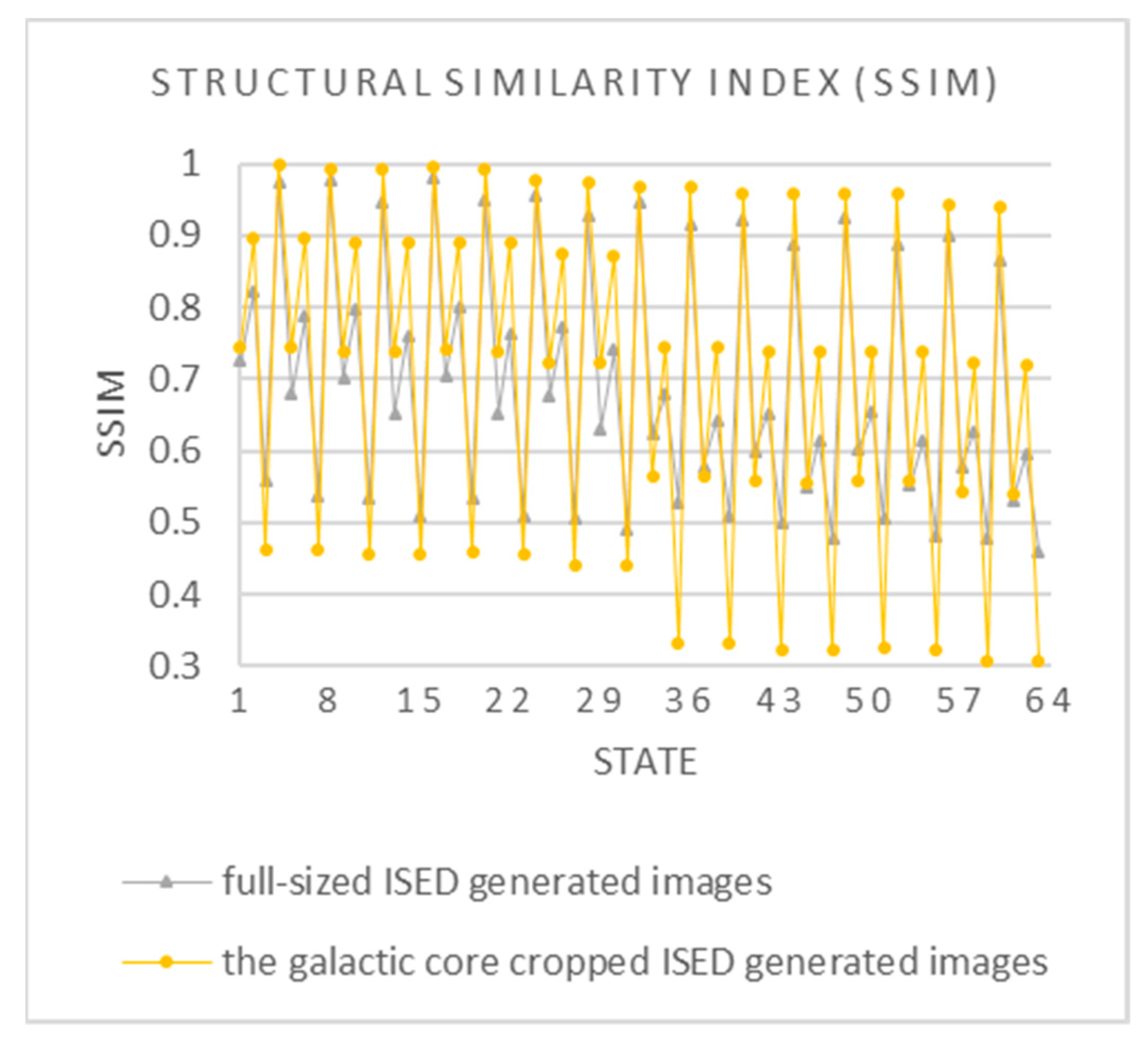
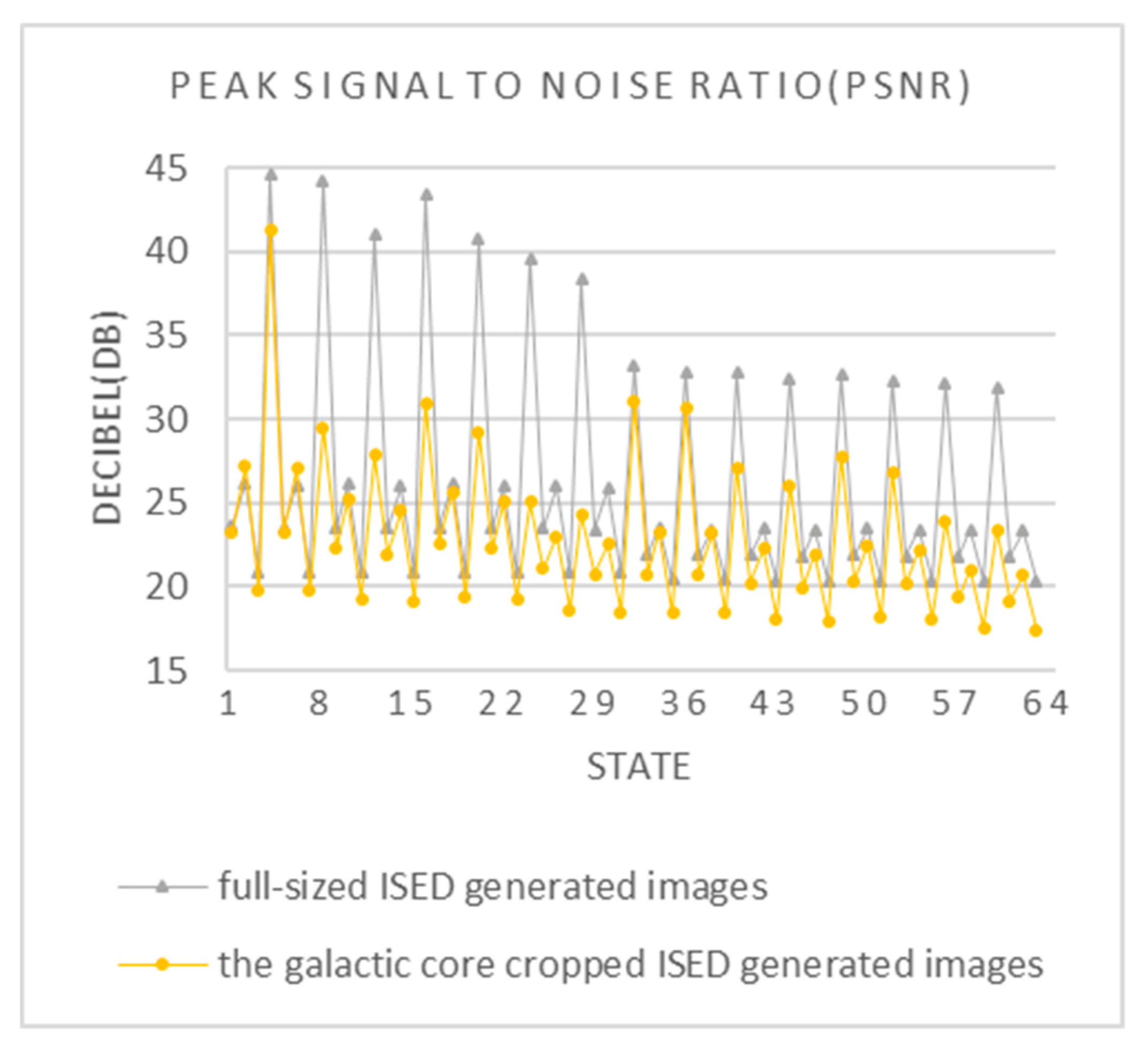
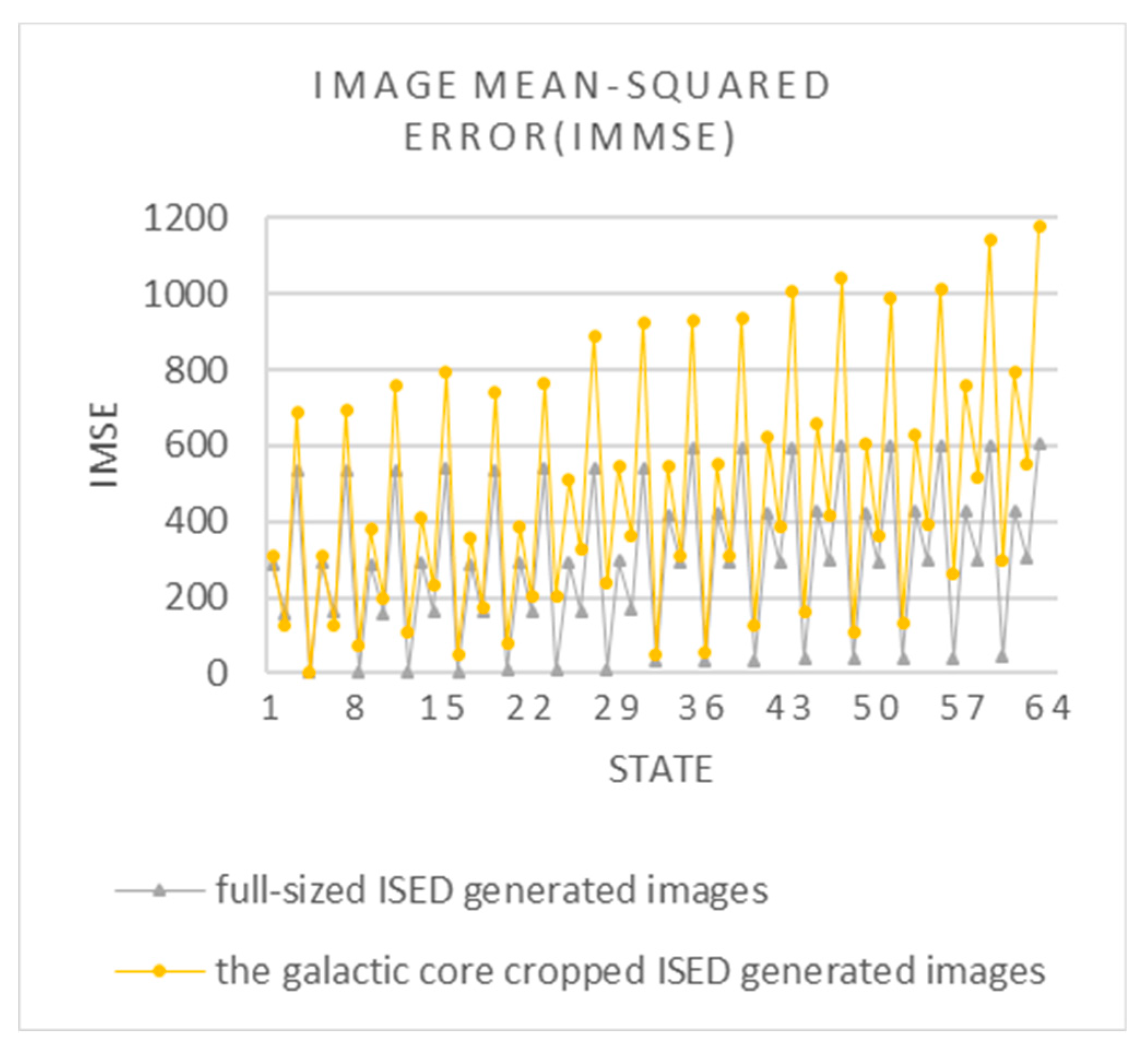
| IQA | SSIM | SSIM | IMMSE | IMMSE | PSNR | PSNR |
| State 1 | 0.7249 | 0.7456 | 284.6252 | 306.8651 | 23.5881 | 23.2613 |
| State 2 | 0.8221 | 0.8974 | 156.2647 | 124.0544 | 26.1922 | 27.1947 |
| State 3 | 0.5578 | 0.4641 | 533.5547 | 687.4574 | 20.859 | 19.7583 |
| State 4 | 0.9729 | 0.9998 | 2.2677 | 4.7465 | 44.5749 | 41.3671 |
| State 5 | 0.6792 | 0.7455 | 289.3453 | 311.6121 | 23.5166 | 23.1947 |
| State 6 | 0.7872 | 0.8972 | 161.0807 | 128.8018 | 26.0604 | 27.0316 |
| State 7 | 0.5376 | 0.4639 | 535.4512 | 692.2054 | 20.8436 | 19.7285 |
| State 8 | 0.9784 | 0.9934 | 2.4546 | 72.9233 | 44.231 | 29.5021 |
| State 9 | 0.7023 | 0.7392 | 287.0798 | 379.7883 | 23.5508 | 22.3354 |
| State 10 | 0.7973 | 0.8908 | 158.7745 | 196.9777 | 26.123 | 25.1866 |
| State 11 | 0.5324 | 0.4577 | 536.0645 | 760.3807 | 20.8386 | 19.3205 |
| State 12 | 0.9456 | 0.9914 | 5.1524 | 105.9679 | 41.0107 | 27.8791 |
| State 13 | 0.6512 | 0.7372 | 292.23 | 412.8335 | 23.4736 | 21.9731 |
| State 14 | 0.7602 | 0.8887 | 163.9132 | 230.0232 | 25.9847 | 24.5131 |
| State 15 | 0.5102 | 0.4557 | 538.2837 | 793.4268 | 20.8207 | 19.1357 |
| State 16 | 0.9813 | 0.9941 | 2.924 | 51.6947 | 43.471 | 30.9963 |
| State 17 | 0.7033 | 0.7405 | 287.8371 | 358.7106 | 23.5393 | 22.5834 |
| State 18 | 0.801 | 0.8916 | 159.1888 | 175.749 | 26.1117 | 25.6819 |
| State 19 | 0.5343 | 0.459 | 536.7666 | 739.3029 | 20.8329 | 19.4426 |
| State 20 | 0.9487 | 0.9925 | 5.4492 | 77.3082 | 40.7675 | 29.2485 |
| State 21 | 0.6523 | 0.7389 | 292.8146 | 384.3246 | 23.4649 | 22.2838 |
| State 22 | 0.7619 | 0.89 | 164.2622 | 201.3634 | 25.9754 | 25.091 |
| State 23 | 0.51 | 0.4575 | 538.9205 | 764.9179 | 20.8156 | 19.2947 |
| State 24 | 0.9564 | 0.9772 | 7.0676 | 203.4258 | 39.6381 | 25.0467 |
| State 25 | 0.6777 | 0.7237 | 291.9807 | 510.4417 | 23.4773 | 21.0513 |
| State 26 | 0.7739 | 0.8747 | 163.3874 | 327.4802 | 25.9986 | 22.979 |
| State 27 | 0.507 | 0.4423 | 540.9653 | 891.0341 | 20.7991 | 18.6319 |
| State 28 | 0.9269 | 0.9751 | 9.495 | 238.2591 | 38.3558 | 24.3603 |
| State 29 | 0.6301 | 0.7216 | 296.8605 | 545.2755 | 23.4053 | 20.7646 |
| State 30 | 0.7409 | 0.8726 | 168.2559 | 362.3143 | 25.8711 | 22.5399 |
| State 31 | 0.489 | 0.4402 | 542.9142 | 925.8688 | 20.7835 | 18.4653 |
| State 32 | 0.946 | 0.9663 | 31.3918 | 50.5701 | 33.1626 | 31.0919 |
| State 33 | 0.6243 | 0.5649 | 417.3726 | 546.6504 | 21.9256 | 20.7537 |
| State 34 | 0.679 | 0.7458 | 289.8595 | 307.8813 | 23.5089 | 23.247 |
| State 35 | 0.528 | 0.3311 | 592.8357 | 931.8355 | 20.4015 | 18.4374 |
| State 36 | 0.9156 | 0.9661 | 33.6595 | 55.3166 | 32.8597 | 30.7022 |
| State 37 | 0.5778 | 0.5648 | 422.0927 | 551.3974 | 21.8767 | 20.7162 |
| State 38 | 0.6434 | 0.7456 | 294.6755 | 312.6287 | 23.4374 | 23.1805 |
| State 39 | 0.5076 | 0.331 | 594.7321 | 936.5834 | 20.3876 | 18.4153 |
| State 40 | 0.9224 | 0.9594 | 34.2917 | 127.0134 | 32.7789 | 27.0923 |
| State 41 | 0.6 | 0.5582 | 420.2725 | 623.0936 | 21.8955 | 20.1853 |
| State 42 | 0.6523 | 0.7389 | 292.8146 | 384.3246 | 23.4649 | 22.2838 |
| State 43 | 0.501 | 0.3244 | 595.7907 | 1008.3 | 20.3799 | 18.095 |
| State 44 | 0.8865 | 0.9573 | 36.9895 | 160.058 | 32.45 | 26.088 |
| State 45 | 0.5482 | 0.5562 | 425.4227 | 656.1388 | 21.8426 | 19.9608 |
| State 46 | 0.6146 | 0.7369 | 297.9534 | 417.3701 | 23.3893 | 21.9256 |
| State 47 | 0.4787 | 0.3224 | 598.01 | 1041.3 | 20.3637 | 17.9549 |
| State 48 | 0.9231 | 0.9596 | 35.5677 | 107.6815 | 32.6202 | 27.8094 |
| State 49 | 0.6028 | 0.559 | 421.4488 | 603.9357 | 21.8834 | 20.3209 |
| State 50 | 0.6541 | 0.7392 | 294.0355 | 364.9927 | 23.4468 | 22.508 |
| State 51 | 0.505 | 0.3252 | 596.9118 | 989.1208 | 20.3717 | 18.1783 |
| State 52 | 0.8874 | 0.958 | 38.0928 | 133.295 | 32.3224 | 26.8827 |
| State 53 | 0.5512 | 0.5574 | 426.4263 | 629.5497 | 21.8324 | 20.1405 |
| State 54 | 0.6144 | 0.7376 | 299.1089 | 390.6071 | 23.3725 | 22.2134 |
| State 55 | 0.4806 | 0.3236 | 599.0657 | 1014.7 | 20.3561 | 18.0673 |
| State 56 | 0.8991 | 0.9425 | 39.6904 | 260.6952 | 32.1439 | 23.9695 |
| State 57 | 0.5783 | 0.542 | 425.5715 | 756.9494 | 21.8411 | 19.3401 |
| State 58 | 0.628 | 0.7222 | 298.2133 | 518.0064 | 23.3855 | 20.9875 |
| State 59 | 0.479 | 0.3083 | 601.0897 | 1142.1 | 20.3414 | 17.5536 |
| State 60 | 0.8667 | 0.9404 | 42.1179 | 295.5284 | 31.8861 | 23.4248 |
| State 61 | 0.5304 | 0.5399 | 430.4513 | 791.7831 | 21.7916 | 19.1447 |
| State 62 | 0.5947 | 0.7201 | 303.0817 | 552.8405 | 23.3152 | 20.7048 |
| State 63 | 0.461 | 0.3062 | 603.0385 | 1177 | 20.3274 | 17.4232 |
| Average | 0.689448 | 0.700152 | 298.2176 | 473.0918 | 26.0371 | 22.83558 |
Appendix C
Table A3.
No Reference IQA.
Table A3.
No Reference IQA.
| M87 | full-size | cropped | full-size | cropped | full-size | cropped |
|---|---|---|---|---|---|---|
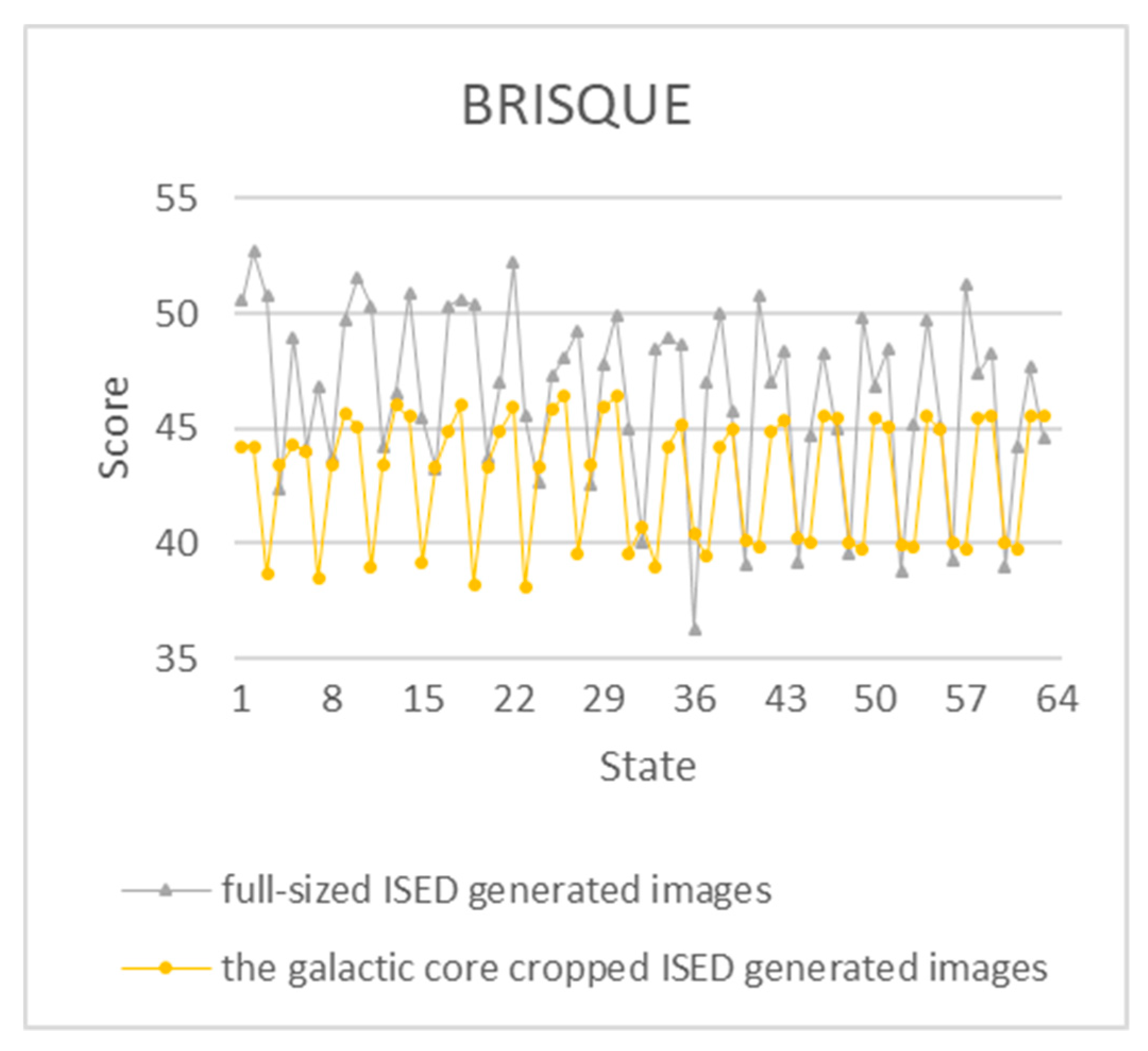
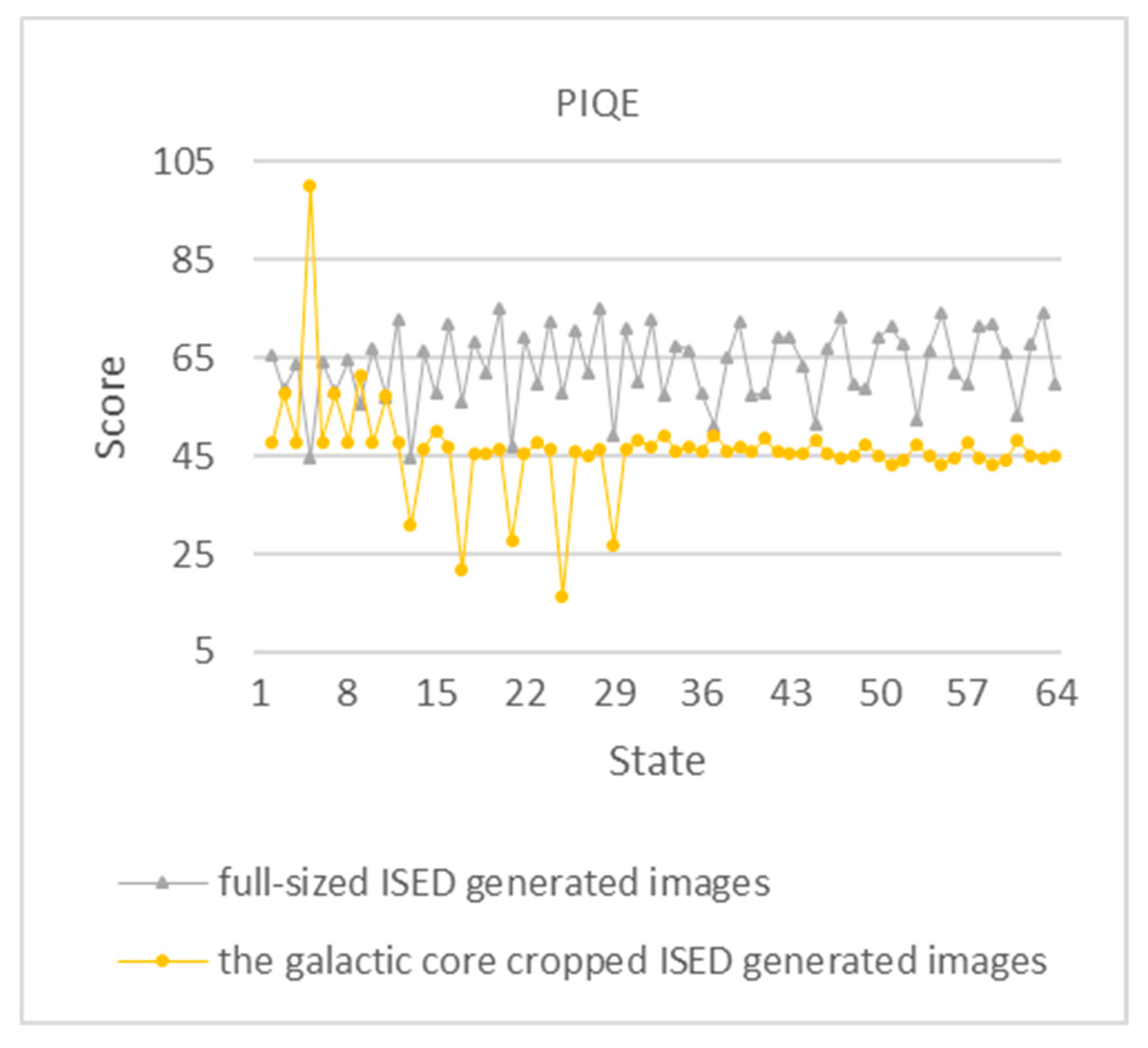
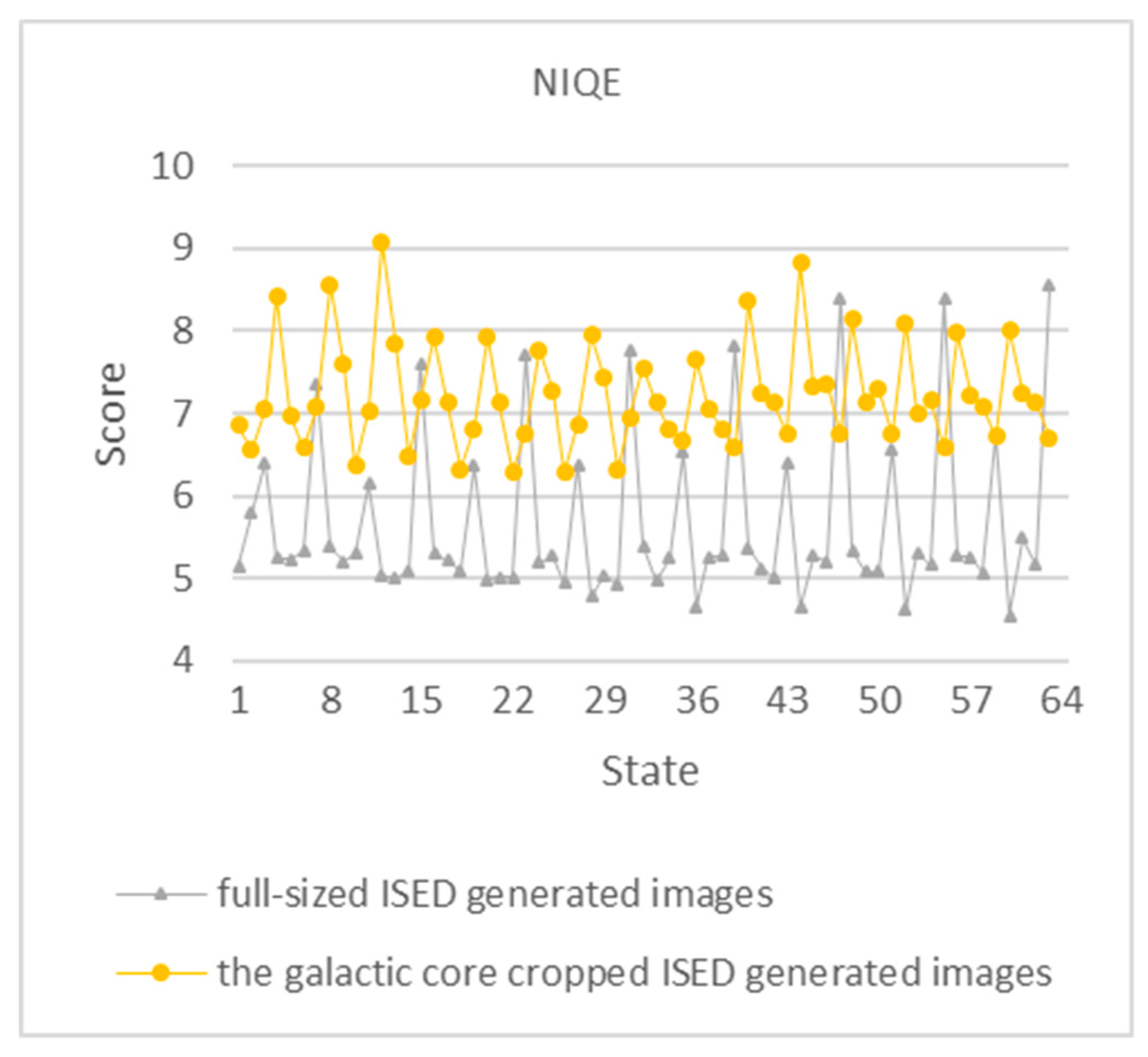
| IQA | NIQE | NIQE | BRISQUE | BRISQUE | PIQE | PIQE |
| Original (0) | 5.5439 | 8.221 | 43.5626 | 43.3802 | 57.3674 | 100 |
| State 1 | 5.1525 | 6.8515 | 50.5449 | 44.2074 | 65.4678 | 47.8352 |
| State 2 | 5.7916 | 6.5504 | 52.7102 | 44.215 | 58.4882 | 57.7265 |
| State 3 | 6.4111 | 7.0434 | 50.7603 | 38.6581 | 63.7614 | 47.9279 |
| State 4 | 5.248 | 8.4311 | 42.3581 | 43.3943 | 44.6338 | 100 |
| State 5 | 5.2352 | 6.9755 | 48.9766 | 44.2729 | 64.315 | 47.8352 |
| State 6 | 5.32 | 6.5772 | 44.1291 | 44.025 | 58.1427 | 57.7265 |
| State 7 | 7.3535 | 7.0815 | 46.8573 | 38.4746 | 64.4827 | 47.9279 |
| State 8 | 5.3848 | 8.5668 | 43.6858 | 43.4027 | 55.6351 | 61.4009 |
| State 9 | 5.2082 | 7.5941 | 49.7429 | 45.6238 | 66.8966 | 47.7678 |
| State 10 | 5.2968 | 6.3655 | 51.5852 | 45.0842 | 57.0669 | 57.3051 |
| State 11 | 6.1516 | 7.0329 | 50.3401 | 38.9643 | 72.8547 | 47.871 |
| State 12 | 5.0405 | 9.0827 | 44.2146 | 43.4156 | 44.798 | 30.8029 |
| State 13 | 4.9928 | 7.8486 | 46.5314 | 46.0398 | 66.2953 | 46.5858 |
| State 14 | 5.0882 | 6.4732 | 50.9033 | 45.5357 | 57.588 | 50.2252 |
| State 15 | 7.6073 | 7.1537 | 45.4138 | 39.1938 | 71.734 | 46.8976 |
| State 16 | 5.3189 | 7.9185 | 43.2691 | 43.3711 | 56.0633 | 21.7746 |
| State 17 | 5.2147 | 7.1367 | 50.3004 | 44.8827 | 68.3096 | 45.588 |
| State 18 | 5.0877 | 6.3235 | 50.6286 | 46.0113 | 61.9339 | 45.6796 |
| State 19 | 6.3632 | 6.8149 | 50.381 | 38.2344 | 75.2535 | 46.1974 |
| State 20 | 4.9809 | 7.9336 | 43.7264 | 43.3744 | 46.701 | 27.6346 |
| State 21 | 5.0113 | 7.135 | 46.9884 | 44.8816 | 69.0178 | 45.5953 |
| State 22 | 5.0051 | 6.2988 | 52.2023 | 45.8963 | 59.7526 | 47.7231 |
| State 23 | 7.7204 | 6.7622 | 45.5546 | 38.0993 | 72.4522 | 46.2034 |
| State 24 | 5.1939 | 7.7798 | 42.6634 | 43.3795 | 57.7926 | 16.4117 |
| State 25 | 5.2773 | 7.2776 | 47.2636 | 45.8317 | 70.7779 | 45.7809 |
| State 26 | 4.9438 | 6.283 | 48.1169 | 46.4452 | 61.9583 | 45.1058 |
| State 27 | 6.3725 | 6.8706 | 49.2368 | 39.5769 | 75.2643 | 46.2315 |
| State 28 | 4.7734 | 7.9567 | 42.573 | 43.3881 | 48.9754 | 26.9581 |
| State 29 | 5.0337 | 7.4362 | 47.7704 | 45.9332 | 70.9652 | 46.5734 |
| State 30 | 4.9093 | 6.3134 | 49.9425 | 46.4059 | 60.0145 | 48.1446 |
| State 31 | 7.7791 | 6.9571 | 44.99 | 39.5976 | 72.8358 | 46.8851 |
| State 32 | 5.396 | 7.554 | 40.0833 | 40.7535 | 57.1412 | 49.3256 |
| State 33 | 4.975 | 7.1325 | 48.4586 | 38.9923 | 67.3844 | 46.1528 |
| State 34 | 5.24 | 6.8071 | 48.9712 | 44.1932 | 66.4844 | 46.7781 |
| State 35 | 6.5276 | 6.6815 | 48.607 | 45.2063 | 57.92 | 45.9668 |
| State 36 | 4.6622 | 7.6449 | 36.3049 | 40.3969 | 51.0752 | 49.3256 |
| State 37 | 5.256 | 7.0666 | 47.0479 | 39.4507 | 65.1939 | 46.1528 |
| State 38 | 5.2697 | 6.8197 | 50.0249 | 44.2262 | 72.371 | 46.7781 |
| State 39 | 7.8122 | 6.5803 | 45.749 | 45.014 | 57.4626 | 45.9668 |
| State 40 | 5.3656 | 8.3644 | 39.1155 | 40.0945 | 57.6231 | 48.6578 |
| State 41 | 5.1239 | 7.2358 | 50.7715 | 39.8505 | 69.2868 | 45.9173 |
| State 42 | 5.0113 | 7.135 | 46.9884 | 44.8816 | 69.0178 | 45.5953 |
| State 43 | 6.4068 | 6.7588 | 48.3767 | 45.3548 | 63.4619 | 45.635 |
| State 44 | 4.6366 | 8.8306 | 39.143 | 40.251 | 51.6093 | 48.2022 |
| State 45 | 5.2678 | 7.3257 | 44.6537 | 40.0555 | 67.1369 | 45.5516 |
| State 46 | 5.2025 | 7.3574 | 48.3003 | 45.5488 | 73.1923 | 44.3819 |
| State 47 | 8.3998 | 6.7453 | 44.9609 | 45.4404 | 59.5353 | 44.9559 |
| State 48 | 5.3462 | 8.1481 | 39.5779 | 40.0773 | 58.6466 | 47.5028 |
| State 49 | 5.0777 | 7.1313 | 49.8544 | 39.7335 | 69.4 | 44.8174 |
| State 50 | 5.0838 | 7.2898 | 46.8529 | 45.4694 | 71.3228 | 43.3041 |
| State 51 | 6.5747 | 6.7488 | 48.4272 | 45.0835 | 67.7667 | 44.2724 |
| State 52 | 4.6214 | 8.1002 | 38.777 | 39.9674 | 52.4489 | 47.4394 |
| State 53 | 5.316 | 6.9881 | 45.1495 | 39.8576 | 66.4963 | 44.9148 |
| State 54 | 5.1681 | 7.1605 | 49.7209 | 45.5227 | 74.0599 | 43.3186 |
| State 55 | 8.3876 | 6.5833 | 45.1085 | 44.95 | 62.0371 | 44.454 |
| State 56 | 5.2763 | 7.9737 | 39.229 | 40.0887 | 59.4569 | 47.7576 |
| State 57 | 5.254 | 7.2237 | 51.2977 | 39.7388 | 71.2543 | 44.6351 |
| State 58 | 5.072 | 7.0904 | 47.4178 | 45.501 | 71.8698 | 43.3825 |
| State 59 | 6.7407 | 6.722 | 48.2777 | 45.5848 | 65.7914 | 44.0943 |
| State 60 | 4.5445 | 8.0195 | 39.0258 | 40.0283 | 53.2504 | 48.1036 |
| State 61 | 5.4902 | 7.2479 | 44.1724 | 39.7898 | 67.779 | 45.1196 |
| State 62 | 5.1631 | 7.1282 | 47.6513 | 45.5478 | 74.2789 | 44.6331 |
| State 63 | 8.5556 | 6.7111 | 44.5938 | 45.5534 | 59.823 | 45.0998 |
References
- Gonzalez, R.; Woods, R. Digital Image Processing, 2nd ed.; Prentice Hall: Upper Saddle River, NJ, USA, 2002; p. 793. [Google Scholar]
- Land, E.H.; McCann, J. Lightness and retinex theory. J. Opt. Soc. Am. 1971, 61, 2032–2040. [Google Scholar] [CrossRef] [PubMed]
- Reinhard, E. High Dynamic Range Imaging: Acquisition, Display, and Image-Based Lighting; Morgan Kaufmann: Burlington, MA, USA, 2006; pp. 233–234. [Google Scholar] [CrossRef]
- Naik, S.; Murthy, C. Hue-preserving color image enhancement without gamut problem. IEEE Trans. Image Process. 2003, 12, 1591–1598. [Google Scholar] [CrossRef] [PubMed]
- Schrödinger, E. An undulatory theory of the mechanics of atoms and molecules. Phys. Rev. 1926, 28. [Google Scholar] [CrossRef]
- Schrödinger, E. Die gegenwärtige situation in der quantenmechanik (the present situation in quantum mechanics). Naturwissenschaften 1935, 23, 807–812. [Google Scholar] [CrossRef]
- Taylor, T. Image State Ensemble Decomposition (ISED). Available online: https://sites.google.com/view/isedisee/home-m87 (accessed on 18 December 2019).
- Einstein, A. Kosmologische betrachtungen zur allgemeinen relativitätstheorie. In Sitzungsberichte der Königlich Preußischen Akademie der Wissenschaften; Phys.-Math. Klasse; Deutsche Akademie der Wissenschaften zu Berlin: Berlin, Germany, 1917; pp. 142–152. [Google Scholar]
- Schwarzschild, K. Über das Gravitationsfeld einer Kugel aus inkompressibler Flüssigkeit nach der Einsteinschen Theorie. In Sitzungsberichte der Königlich Preussischen Akademie der Wissenschaften zu Berlin; Phys.-Math. Klasse: Berlin, Germany, 1916; pp. 424–434. [Google Scholar]
- Thorne, K. Black Holes and Time Warps: Einstein’s Outrageous Legacy; W.W. Norton: New York, NY, USA, 1994. [Google Scholar] [CrossRef]
- Webster, B.L.; Murdin, P. Cygnus X-1-a Spectroscopic Binary with a Heavy Companion? Nature 1972, 235, 37–38. [Google Scholar] [CrossRef]
- Bolton, C. Identification of Cygnus X-1 with HDE 226868. Nature 1972, 235, 271–273. [Google Scholar] [CrossRef]
- The EHT Collaboration. First M87 event horizon telescope results. IV. Imaging the central supermassive black hole. Astrophys. J. Lett. 2019. [Google Scholar] [CrossRef]
- Jet Propulsion Laboratory California Institute of Technology Spitzer Space Telescope. Available online: http://www.spitzer.caltech.edu/images/6596-ssc2019-05c-Spitzer-Captures-Messier-87 (accessed on 28 November 2019).
- Maxwell, J.; Gabriel, S. On the theory of compound colours, and the relations of the colours of the spectrum. Phil. Trans. R. Soc. 1860, 150, 57–84. [Google Scholar] [CrossRef]
- Rector, T.; Levay, Z.; Frattare, L.; Arcand, K.; Watzke, M. The aesthetics of astrophysics: How to make appealing color-composite images that convey the science. Astron. Soc. Pac. 2017, 129, 975. [Google Scholar] [CrossRef]
- Gibbs, J. Elementary Principles in Statistical Mechanics; Charles Scribner’s Sons: New York, NY, USA, 1902. [Google Scholar]
- Einstein, A. Concerning an heuristic point of view toward the emission and transformation of light. Ann. Phys. 1905, 17, 132–148. [Google Scholar] [CrossRef]
- Bohr, N. The quantum postulate and the recent development of atomic theory. Nature 1928, 121, 580. [Google Scholar] [CrossRef]
- Einstein, A.; Infeld, L. The Evolution of Physics: The Growth of Ideas from Early Concepts to Relativity and Quanta; Cambridge University Press: Cambridge, UK, 1938. [Google Scholar]
- Mandel, L.; Wolf, E. Optical Coherence and Quantum Optics; Cambridge University Press: Cambridge, UK, 1995. [Google Scholar] [CrossRef]
- Zhou, W.; Bovik, A.; Sheikh, H.; Simoncelli, E. Image quality assessment: From error visibility to structural similarity. IEEE Trans. Image Process. 2004, 13, 600–612. [Google Scholar] [CrossRef]
- Venkatanath, N.; Praneeth, D.; Chandrasekhar, B.; Channappayya, B.S.; Medasani, S. Blind image quality evaluation using perception based features. In Proceedings of the 21st National Conference on Communications (NCC), Mumbai, India, 27 February–1 March 2015. [Google Scholar] [CrossRef]
- Sheikh, H.; Wang, Z.; Cormack, L.; Bovik, A. LIVE Image Quality Assessment Database Release 2. Available online: https://live.ece.utexas.edu/research/quality (accessed on 28 November 2019).
- Mittal, A.; Soundararajan, R.; Bovik, A. Making a completely blind image quality analyzer. IEEE Signal Process. Lett. 2013, 22, 209–212. [Google Scholar] [CrossRef]
- Mittal, A.; Moorthy, A.; Bovik, A. No-reference image quality assessment in the spatial domain. IEEE Trans. Image Process. 2012, 21, 4695–4708. [Google Scholar] [CrossRef] [PubMed]
- Mittal, A.; Moorthy, A.; Bovik, A. Referenceless image spatial quality evaluation engine. Presentation at the 45th Asilomar Conference on Signals, Systems and Computers, Pacific Grove, CA, USA, 6–9 November 2011. [Google Scholar] [CrossRef]
- Willett, K.; Galloway, M.; Bamford, S.; Lintott, C. Galaxy zoo: Morphological classifications for 120,000 galaxies in hst legacy imaging. Mon. Not. R. Astron. Soc. 2016, 464. [Google Scholar] [CrossRef]
- Feynman, R. Lectures in Physics, Vol. 1; Addison Wesley Publishing Company Reading: Boston, MA, USA, 1963; pp. 30–31. [Google Scholar]
© 2020 by the authors. Licensee MDPI, Basel, Switzerland. This article is an open access article distributed under the terms and conditions of the Creative Commons Attribution (CC BY) license (http://creativecommons.org/licenses/by/4.0/).