High-Strain-Rate Compressive Behavior of UHMWPE Fiber Laminate

Abstract

Ultra-high-molecular-weight polyethylene (UHMWPE) fiber laminate is currently widely used in ballistic protection for its exceptional physical and mechanical properties. However, the dynamic compressive mechanism of UHMWPE laminate remains poorly understood. Therefore, the stress–strain relationship, the influence of different thickness, area, and shape, and the maximum stress and fracture stress are studied in both out-of-plane and in-plane directions under quasi-static and dynamic loading using a universal test machine, Split Hopkinson pressure bar (SHPB), and high-speed camera. Furthermore, numerical models with cohesive elements are developed. The results indicate a dependency on strain rate and loading direction. Firstly, the stress–strain curve of dynamic testing can be divided into different zones according to different loading directions and strain rates. Secondly, with the increase of the strain rate in the dynamic testing, the maximum stress and fracture stress increase as well; relatively speaking, the fracture stress in the out-of-plane direction is greater than the fracture stress in the in-plane direction. Thirdly, both experiment and simulation indicate that the thickness does not influence the modulus clearly the in out-of-plane direction but influences the modulus in the in-plane direction. Fourthly, the fracture stress of dynamic testing is higher than the fracture stress of quasi-static testing in both directions. Finally, the numerical results show good agreement with the experiment in terms of the maximum stress and failure form.

1. Introduction

The combination of ductile materials and brittle materials can result in a lightweight material, which prevents penetration and effectively protects the human body [1,2]. Fiber-reinforced composite laminate is suitable for protection against higher-lethality fragmentation threats [3]. Therefore, fiber-reinforced laminate behind ceramic could perform significantly as a ductile material in protecting a human torso [4,5,6]. In addition, fiber-reinforced laminate could also be made into a protective helmet as a weight-critical application [3].

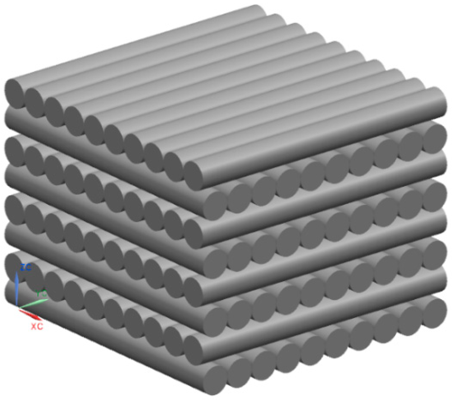
Ultra-high-molecular-weight polyethylene (UHMWPE) fiber has exceptional physical and mechanical properties, such as high impact resistance, high wear resistance, high chemical resistance, and low friction coefficient [7]. Therefore, it is widely used in ballistic protection, as well as the aerospace and military industries [8,9]. In typical UHMWPE ballistic composite sheets, unidirectional (UD) layers of fibers are impregnated with a thermoplastic matrix, and they are stacked in 0°/90° arrangement [10]. For flexible applications like ballistic vests, UD layers are covered on both sides with a thin polymer film [10] and stacked to become a laminate as shown in Figure 1. This structure gives far better protection than fabrics with the same weight [11]. There were many experiments and numerical simulations studying the impact response of UHMWPE laminate [12,13,14,15]; however, the mechanics of resisting impact threats remains poorly understood [16].

To achieve the necessary understanding of the mechanics of resisting impact, it is essential to study the dynamic compressive properties of UHMWPE fiber-reinforced laminate. Moreover, the methods applied in testing other fiber-reinforced composites are necessary as important references.

For other fiber composites, Arbaoui [17] studied the compressive material properties and damage kinetics of cubic specimens of [0°/90°]₂₆ (26 repetitions of [0°/90°] stack) woven E-glass/vinyl ester laminate in the in-plane and out-of-plane directions from low to high strain rates. The results showed that a higher strain rate led to a higher maximal stress level. In addition, the maximal stresses obtained during dynamic compression tests were higher for the composite subjected to in-plane loading than for that subjected to out-of-plane loading at the same strain rate. Moreover, the specimens were mainly damaged in a crushing and shear failure mode under out-of-plane loading; as for the in-plane test, the failure was dominated by fiber buckling and delamination. Pankow [18] evaluated the rate dependence of the through-the-thickness and in-plane compression response of a three-dimensional (3D) 6% Z-fiber woven composite (3DWC). It was found that 3DWC showed an increase in strength in all three directions studied. In the warp and weft directions, the material had a clear transition in the failure mode dominated by kink band formation at low rates to delamination at much higher rates.

For UHMWPE woven composites, Ying [19] studied the compressive stress–strain curve, strain at yield stress, and impact energy absorption of UHMWPE/vinyl ester 2.5D angle interlocked woven composites under three high strain rates (360, 710, and 1120 s⁻¹) and quasi-static compression. The results showed that the yield stress, strain at yield stress, and modulus all increased with the increased strain rate. Kai [20] studied the dynamic compressive properties of UHMWPE interlaced biaxial weft knitted (IBWK) fabrics/vinyl ester resin composites. The results showed that the peak stress, compressive modulus, and specific fracture strain energy density increased with the increase in strain rate.

For UHMWPE laminate, Shi [21] studied the dynamic mechanical properties of UHMWPE fiber-reinforced composites with three different laminated angles (0°/90°, 0°/90°/45°/−45°, 0°/90°/30°/−60°/60°/−30°) at higher strain rates under out-of-plane compression. The energy absorption capabilities were sensitive to the laminated angle of composites under medium-velocity impact. In addition, delamination and compaction in the thickness direction constituted the main dynamic failure mechanisms. Asija [22] investigated both shear thickening fluid (STF)-treated and neat gold shield UHMWPE composites specimens subjected to high-strain-rate impact using Split Hopkinson pressure bar (SHPB) experiments. He studied the properties of the neat specimens under strain rates from 3120 to 13,100 s⁻¹ and the STF-treated specimens under strain rates from 5000 to 15,600 s⁻¹. The results showed that the peak stress increased as the strain rate increased. Moreover, the STF-treated gold shield specimens exhibited higher values of specimen peak stress, peak strain, specimen strain rate, and impact toughness as compared to the neat untreated specimens.

In terms of simulations, there were some studies on the quasi-static compression [23], interlaminar shear [24,25], and ballistic impact responses of UHMWPE laminate [14,23]. Nguyen [23] developed finite element (FE) models to verify mechanical test results under out-of-plane compression and got good agreement. Bogetti [24] developed FE models and applied a surface-based traction–separation contact condition to simulate the nonlinear and unloading material behavior measured by digital image correlation (DIC). Lässig [14] developed an FE model for simulating a panel with AD (areal density) = 15 kg/m² impacted by a 6-mm-diameter aluminum sphere at a velocity of 3532 m/s. The results showed good agreement on the height and width of the ejecting debris cloud on the back face when compared with the ballistic experiment. Then, validation simulations of seven impact situations for an impact velocity range of 2052 m/s to 6591 m/s also showed good applicability and realistic perforation predictions in terms of the impact velocity–residual velocity relationship. Nguyen [23] applied a new sub-laminate discretization approach to more accurately capture out-of-plane failure. The model was extensively validated using experimental ballistic data for a wide range of UHMWPE target thicknesses up to 102 mm against 12.7-mm and 20-mm caliber fragment simulating projectiles (FSPs) with impact velocities between 400 m/s and 2000 m/s. Very good overall agreement with experimental results was seen for depth of penetration, ballistic limit, and residual velocity, while the penetration mechanisms and target bulge behavior were accurately predicted. In terms of studies looking at the matrix individually, Grujicic [26] built a cell unit containing a fiber model, matrix model, and cohesive elements between them. Chocron [27] modeled polyurethane matrix material into a strip, which, in the example, took 20% of the space in volume and was placed side by side with the fiber “bundle”. However, the simulation of high-strain-rate compression of UHMWPE laminate is less studied than other kinds of fiber laminate [17,28].

In terms of ballistic protection, there were some studies looking at smart materials and other fibers used. Smart materials like shear thickening fluid (STF) are used to enhance impact resistance. This smart fluid increases its viscosity under applied loadings and exhibits a solid-like state for a split second since the loading reaches upper levels [29]. It was observed that areal density, flexibility, and thickness of the fabric remain almost the same after STF treatment, but there is significant enhancement in the magnitude of impact energy absorption [30]. For other fibers, Simić [31] studied the ballistic and stab performance of composite material based on aramid fabric and polyvinyl butyral (PVB), reinforced by adding a small concentration of inorganic nanotubes of tungsten disulfide (INT-WS2). A significant improvement in anti-ballistic performance was observed: 39.3% higher impact toughness, 8.5% higher absorbed energy of stab, and 12% smaller depth of back-face deformation after shots. Li [32] studied the numerical back-face deformation of Kevlar fiber helmet under ballistic impact at different locations and in different directions. The results showed good agreement with the experiment conducted by Reference [33] using the DIC technique.

To sum up, current dynamic compressive tests of fiber composites focus on the maximum stress or failure stress, absorbed energy, and damage kinetics with the increase in strain rates [34,35]. Studies on UHMWPE fiber-reinforced composite laminate are less common than studies on other fiber composite laminates. Moreover, investigations of both out-of-plane and in-plane directions are also important. However, many studies on UHMWPE laminate mainly focused on the out-of-plane direction; the in-plane properties were not explored as carefully as for other fiber composites [17,18]. In addition, the size and the shape of the specimen had an influence on the dynamic properties in many studies [7,36,37,38]. Thus, the effect of size and shape with regard to UHMWPE laminate should also be explored [14].

Therefore, in order to explore the items mentioned above, a careful, systematic study of the dynamic compressive mechanical properties of UHMWPE fiber-reinforced composite laminate is of importance.

In this study, quasi-static and dynamic compression mechanical experiments of specimens under both out-of-plane and in-plane directions were conducted using a universal test machine, SHPB, and high-speed camera. At first, for the quasi-static experiment, the stress–strain relationships under both directions were studied. Then, for the dynamic experiment, four aspects were studied. Firstly, the stress–strain curve was divided into several zones according to different characteristics. Secondly, the change in maximum stress, fracture stress, and energy absorption with the increase in strain rate were studied. Thirdly, the influences of thickness, area, and shape of the specimens on the stress–strain relationship were studied. Fourthly, the tendency of fracture stress in terms of quasi-static and dynamic properties is studied. Finally, FE models with cohesive elements were developed to support the experimental findings by comparing the maximum stress values and delamination form.

2. Experimental Procedure

2.1. Material and Specimens

The material studied here was the UHMWPE fiber-reinforced polyurethane matrix laminate manufactured by the Ningbo Dacheng Advanced Material Co., Ltd. in Ningbo city, Zhejiang province of China. The area average density was 9.7 kg/m². The thickness was 11 mm. The diameter of the fiber was about 25 μm. The density of the polymer matrix was around 1.1 × 10³ kg/m³, and the volume fraction was around 20%. The structure of this laminate involved a layer of 0°-direction fibers covered by a layer of 90°-direction fibers, as shown in Figure 1. This structure is usually designed for stiff applications like helmets and panels [10]. Due to its cross-ply layup, the laminate is assumed to be orthotropic [22]. Therefore, the material properties of 0°- and 90°-directions were taken to be equal. As shown in Figure 1, the xc- or yc-direction was taken as the in-plane direction, whereas the zc-direction was taken as the out-of-plane direction.

The laminate was firstly manufactured as a 1.2 × 1.6 m plate and then cut into a 250 × 300 mm plate. To make sure the properties inside the specimens were uniform and consistent, it was necessary to make the specimens while abiding to four rules as best as possible. Firstly, small pieces were cut by water jet from the smaller plate at a distance away from the edge of more than 15 mm. These pieces had the same cross-section as the final specimen but they all had a thickness of 11 mm. Secondly, one small piece could be used to make one 5-mm specimen or two 3- or 4-mm specimens. Thirdly, all specimens were taken from one plate, or at least from plates in the same batch. Fourthly, to ensure that the sizes of the upper and lower faces of the specimens were similar to an acceptable degree, the water jet was moved slowly.

Various sizes of cylindrical and cuboid specimens were made for study as presented in

Table 1. The sizes of the specimens.

Direction	Load	Diameter × Thickness/Length × Width × Thickness
		(mm × mm/mm × mm × mm)
Out-of-plane	Quasi-static	20 × 20 × 10, 8 × 8 × 4
	Dynamic	Φ10 × 5, Φ10 × 4, Φ10 × 3, Φ9 × 4, Φ8 × 4, 8 × 8 × 4
In-plane	Quasi-static	10 × 20 × 20, 8 × 8 × 8
	Dynamic	4 × 8 × 8, 8 × 8 × 8, 8 × 8 × 5

. The underlined number represents the value of the loading direction.

2.2. Test Apparatus

2.2.1. Quasi-Static Test

The quasi-static uniaxial tests were performed on a universal testing machine. The electronic universal testing machine CMT6000 (MTS Systems Corporation, Eden Prairie, Minnesota of USA) for in-plane compression has a maximum loading capacity of 5 kN. The electronic universal testing machine CSS-44100 (Changchun Research Institute for Testing Machines, Changchun city, Jilin Province of China) for out-of-plane compression has a maximum loading capacity of 300 kN. The loading speed was 2 mm/min. Thus, the strain rates for different thicknesses (10, 4, 20, and 8 mm) were 3.33 × 10⁻³, 8.33 × 10⁻³, 1.67 × 10⁻³, and 4.16 × 10⁻³ s⁻¹, respectively, according to $\dot{\epsilon }=v/l_s$, where $v$ is the loading speed and $l_s$ is the thickness of specimen. The specimen under quasi-static loading was preferably cuboid, because a cylindrical specimen easily loses stability during the compression process.

2.2.2. Dynamic Test

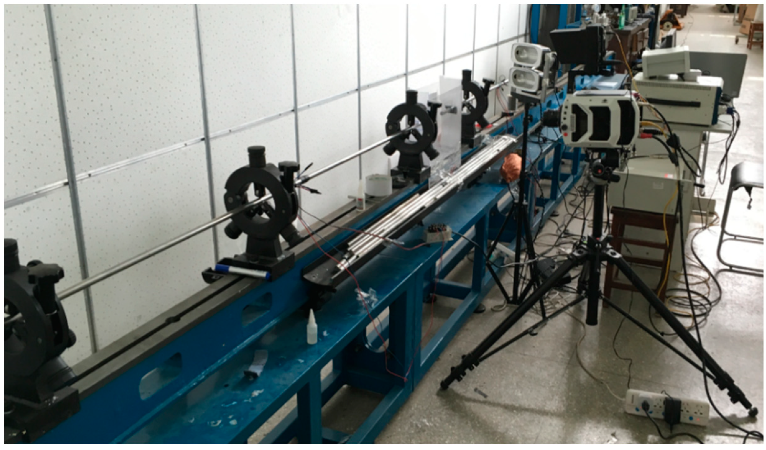
The Split Hopkinson pressure bar (SHPB) apparatus is widely applied to study the dynamic behavior in strain rates ranging from 100–10,000 s⁻¹ [39]. Due to the different hardness in the out-of-plane and in-plane directions, steel bars and aluminum bars were applied, respectively. The values of density and Young modulus for the steel and aluminum bars were 7.85 × 10³ kg/m³, 206 GPa and 2.8 × 10³ kg/m³, 72 GPa, respectively. The striker bar had a length of 0.4 m for aluminum and 0.5 m for steel. The input and output bars had lengths of 1.5 m and 1.5 m, respectively. Their diameters were all 14.5 mm. In addition, a Φ10 × 1 mm copper thin circular slice and a Φ10 × 1 mm thin circular hard paper slice were used as the pulse shapers for the out-of-plane and in-plane compression, respectively. For each experiment, a fresh pulse shaper was used [22,40]. The recording of stress waves was performed using a pair of two half bridges that compensated for the bending effect of the bars [41], as shown in Figure 2. To reduce the non-uniform stress distribution due to friction [42,43,44], Vaseline was applied to the two contact faces of each specimen. The SHPB apparatus (Luoyang Liwei Technology Co., Ltd., Luoyang city, Henan province of China) is shown in Figure 3; a high-speed camera (Phantom V2511, Vision Research, Inc., Wayne, New Jersey, USA) was applied to record the morphology under high-strain-rate loading [18].

Upon impact of a projectile at the free end of the input bar, a compressive longitudinal incident wave ${\epsilon }_i$ in the input bar is developed. This incident wave induces a reflected wave ${\epsilon }_r$ in the input bar and a transmitted wave ${\epsilon }_t$ in the output bar [17]. The stress–strain curve of the specimen can be calculated from the forces and the velocities at both specimen faces. The classical calculation is based on the hypothesis of homogeneity of stress and strain within the specimen [17]. The calculation equations are in the form of Equations (1)–(3) [17,22,28], where $l_s$ and $A_0$ are the thickness and area of the specimen, while $c$, $A$, and $E$ are the sound speed, area, and Young modulus of bar. The energy absorption can be calculated using Equation (4) [21].

$$\dot{\epsilon }\left(t\right)=\frac{c}{l_s}\left({\dot{\epsilon }}_i-{\dot{\epsilon }}_r-{\dot{\epsilon }}_t\right).$$

(1)

$$\epsilon \left(t\right)=\frac{c}{l_s}{{\displaystyle \int }}_0^t\left({\epsilon }_i-{\epsilon }_r-{\epsilon }_t\right)dt.$$

(2)

$$\sigma \left(t\right)=\frac{A}{2A_0}E\left({\epsilon }_i+{\epsilon }_r+{\epsilon }_t\right).$$

(3)

$$W=AEc{{\displaystyle \int }}_0^t\left[{\epsilon }_i{\left(t\right)}^2-{\epsilon }_r{\left(t\right)}^2-{\epsilon }_t{\left(t\right)}^2\right]dt.$$

(4)

Furthermore, when it comes to aligning the wave head, there are many methods. Shang [45] considered that, when changing the position of the three wave heads, if the stress–strain curves generated by the two-wave method and three-wave method could be aligned at the maximum strain point, the head of the three waves could be considered as aligned. Some researchers calculated the wave head differences by measuring the distances between the strain gages and the ends of the bars in contact with the specimen, as well as by measuring the wave speed of the bars and evaluating the wave speed of the specimen [46]. Under ideal conditions, this method could get more accurate results. However, if the wave speed of the specimen is not clear enough [47] or the measurements of the lengths are not accurate enough, applying the same value for each specimen could lead to the result of each specimen being inaccurate. The method applied here was as follows: when changing the position of the reflected and transmitted waves, if the standard deviation of ${\epsilon }_t-\left({\epsilon }_i+{\epsilon }_r\right)$ was the minimum, the head of the three waves could be considered as aligned.

3. Experimental Results and Discussion

3.1. Out-of-Plane Test

3.1.1. Quasi-Static Compression

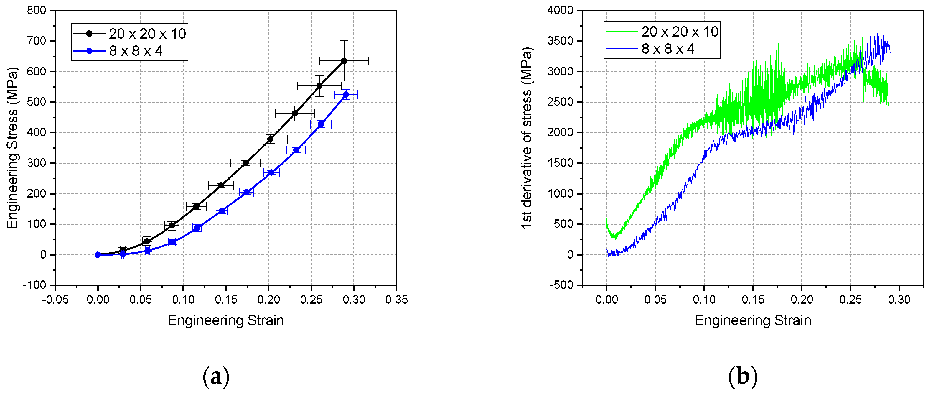
Two sizes of specimens were studied. The loading speed was 2 mm/min; thus, the strain rate for the 20 × 20 × 10 specimen was 3.37 × 10⁻³ ± 8.0408 × 10⁻⁶ s⁻¹, and the strain rate for the 8 × 8 × 4 specimen was 8.31 × 10⁻³ ± 5.4029 × 10⁻⁵ s⁻¹. Firstly, as shown in Figure 4a, the fracture stress of the bigger specimen was higher, while the fracture strain values of the two sizes of specimens were similar, i.e., 2.8861 × 10⁻¹ ± 2.895 × 10⁻² and 2.9064 × 10⁻¹ ± 1.366 × 10⁻², respectively. Secondly, as obviously shown in Figure 4b, there were two phases during the loading. The first phase possibly represents the compact procedure, where the pores among the specimen were compressed outward. The second phase possibly represents the bearing procedure, where the fibers began holding the load. The bigger specimen could hold the loading more stably, and it seems that the bigger specimen became stable more quickly during the first phase. As shown in Figure 4a, the compressive strength of the 20 × 20 × 10 specimen was 634.8947 ± 66.3778 MPa, which is similar to the compressive strength of ~650 MPa in Reference [4] using the same size of specimen.

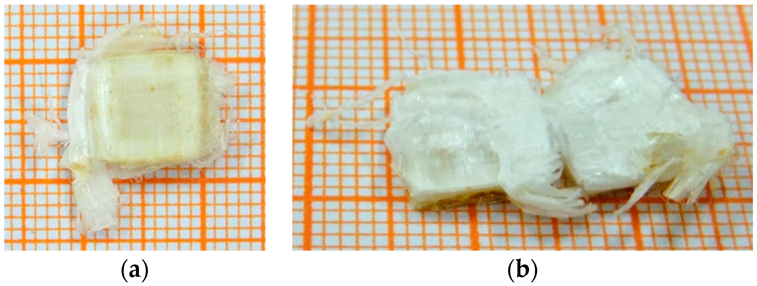
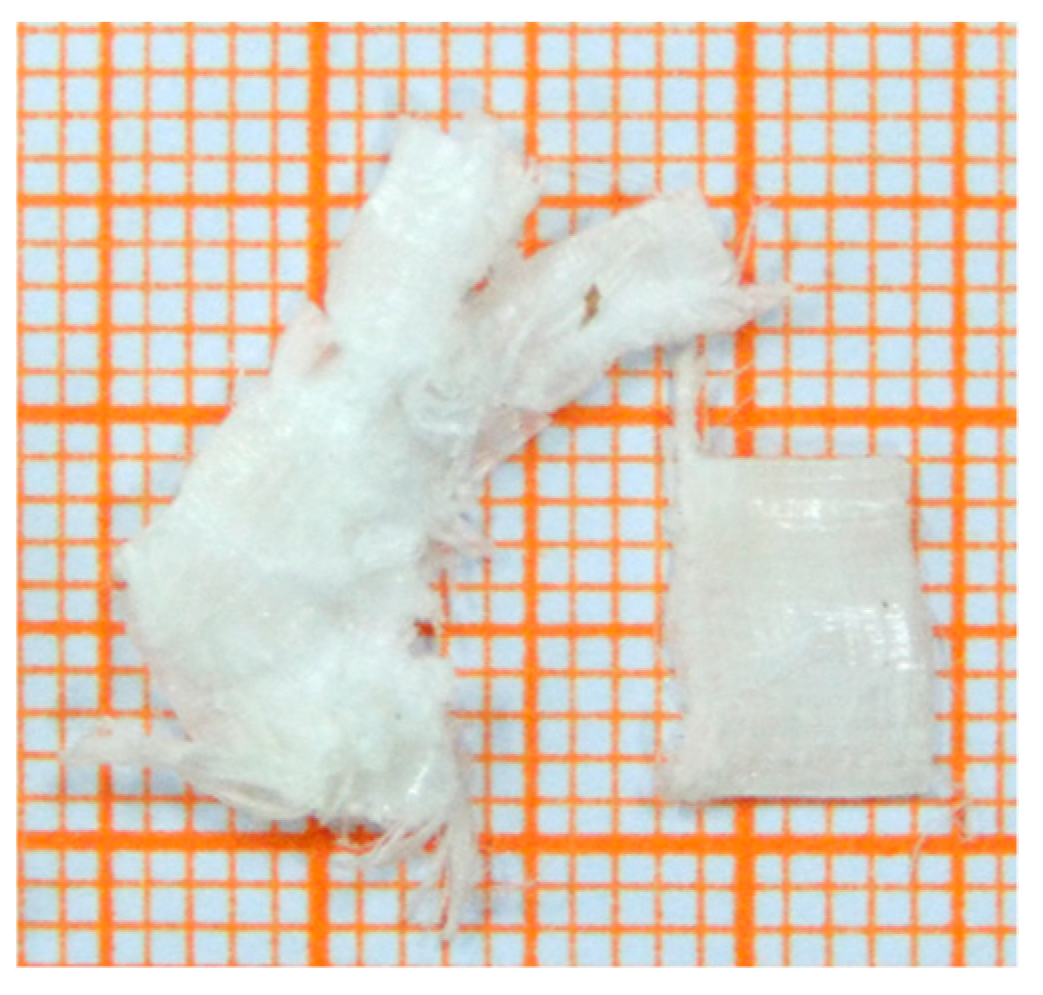
As shown in Figure 5, the specimens had a shear failure feature. As shown in Figure 5a and Figure 6a, many fibers were squeezed out along the four edges of the specimen and, thus, a little square was presented at the center of the surface. Therefore, an inner shear generated in some places, which resulted in the fibers being cut off as shown in Figure 5b and Figure 6b. Another feature is that, when failure occurred, there was always a loud popping sound like an explosion, and the pieces of fibers splashed all over the place.

3.1.2. Dynamic Compression

(a) Mechanical Behavior

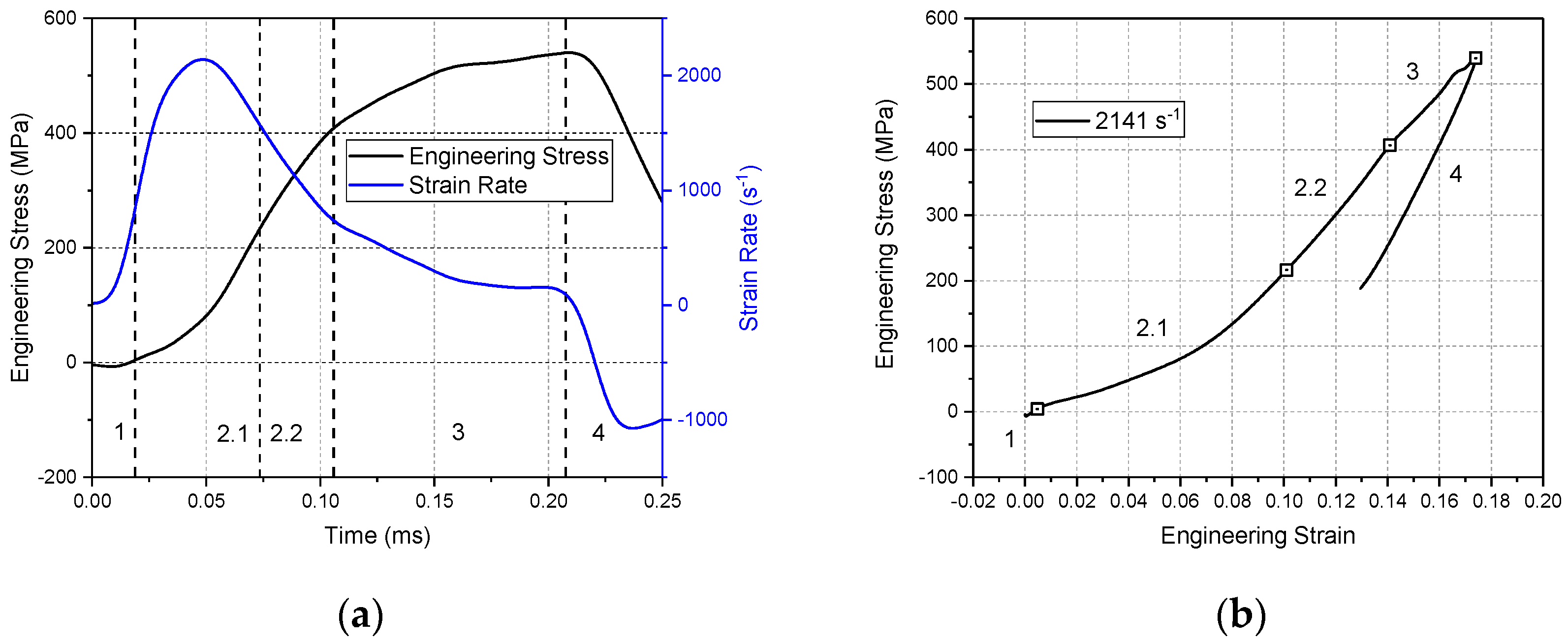
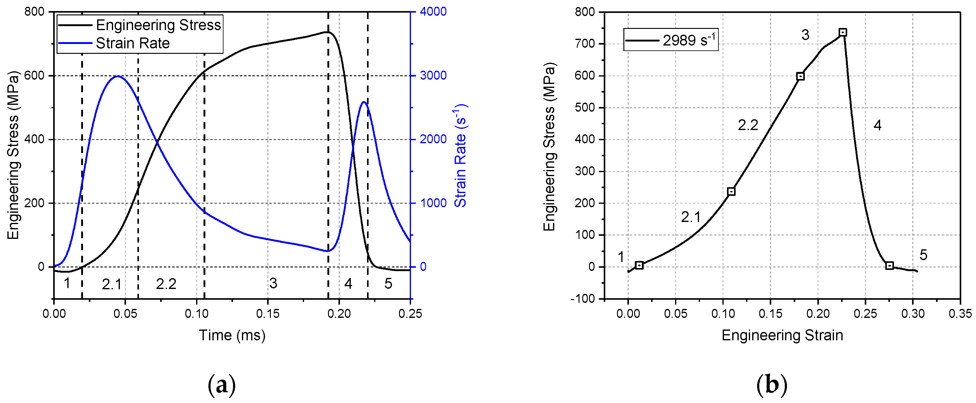
For the non-damaged tests of the Φ9 × 4 specimen under 0.4 MPa, shown in Figure 7, the stress–strain curve could be divided into four zones [17].

Zone 1: This period is called the self-installation zone. The strain rate increased rapidly, but the stress fluctuated around 0. This is because the parallelism of the specimen faces in contact with the bars was not 100% guaranteed.

Zone 2: This period is called the under-loading zone. Once the perfect contact was ensured, the strain rate began to drop. As the strain rate increased, the stress increased as well. However, the stress–strain relationship showed two different periods in this zone. During the 2.1 period, the stress–strain curve was not linear, possibly due to the pores among the specimen being compressed. During the 2.2 period, the stress–strain curve was linear and stable, due to the material being more uniform with the specimen yet to be damaged.

Zone 3: This period is called the soften zone. The strain rate tended to zero and the stress tended to an average value. The stress reached the maximum value when the strain rate reached zero. As shown in Figure 7b, the material behavior showed a softening phenomenon.

Zone 4: This period is called the spring-back zone. The strain rate changed sign, and the stress started to decrease. The specimen began to relax and then recovered. This shows that, even though several fibers were squeezed out, the main body of the specimen suffered no serious damage. Therefore, the specimen still had the ability to spring back.

For the damaged tests of the Φ9 × 4 specimen under 0.8 MPa, shown in Figure 8, the stress–strain curve could be divided into five zones [17].

Zone 1 and Zone 2 were the same as those for the non-damaged tests.

Zone 3: This period is called the soften zone. As shown in Figure 8b, there was serious fluctuation in the stress curve. This was possibly because the microscopic damage under higher strain rate was more serious than that under lower strain rate.

Zone 4: This period is called the fracture zone. The accumulation of microscopic damage resulted in the appearance of a macroscopic defect. The fracture of the material generated a rapid fall in the stress with a rapid increase in the strain rate. The presence of a second peak characterized the onset of macroscopic damage [48]

Zone 5: This period is called the compact zone. The damaged specimen became more compact; the rest of the specimen could hold the loading temporarily, which caused a sharp drop in the strain rate. It is obvious that the spring-back behavior disappeared.

(b) Damage Kinetics

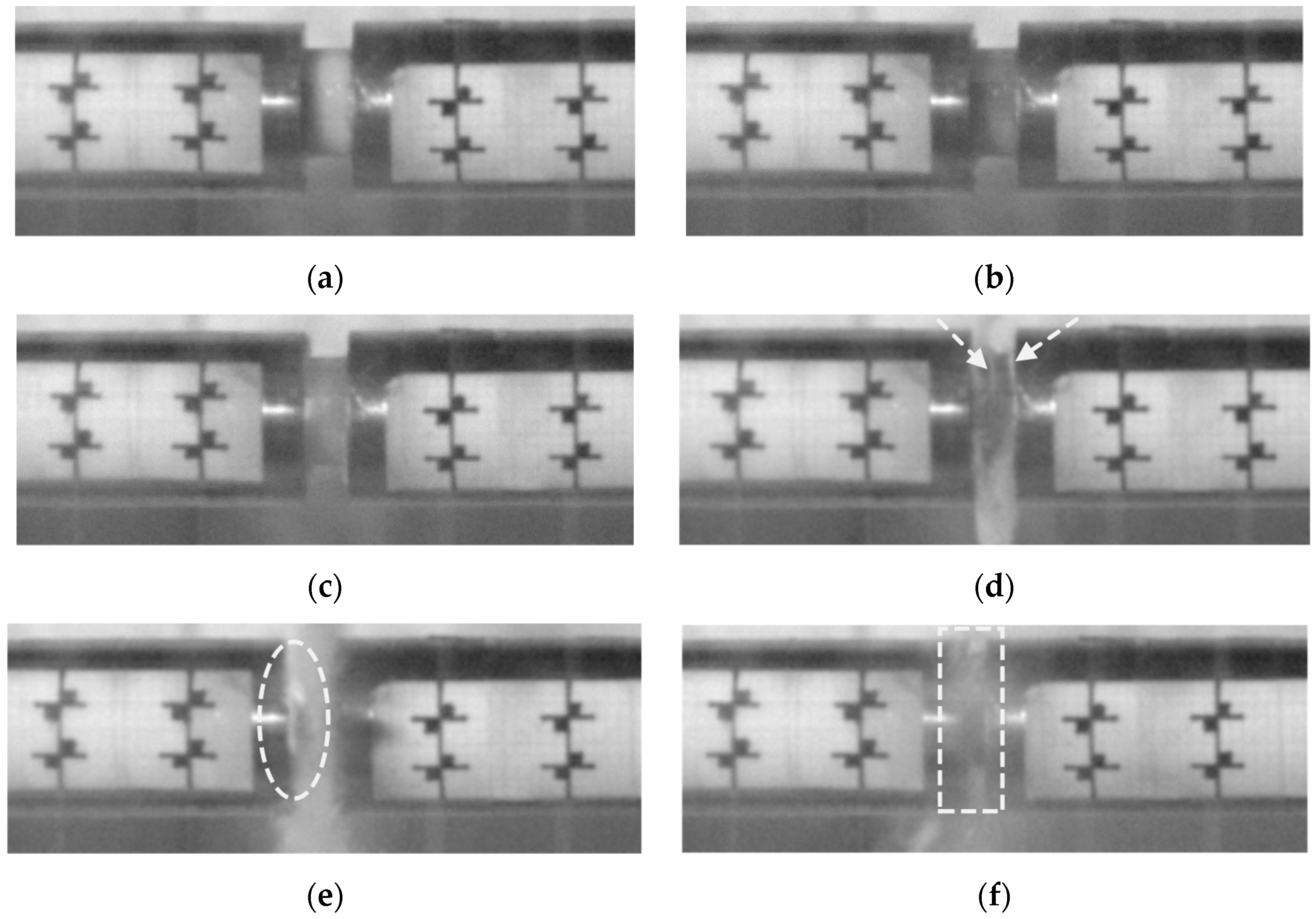
The high-speed camera records show that some fibers were squeezed out from the sides during the loading before the specimen was damaged completely, which can be seen in Figure 9. This is because the specimens were made of 0°/90° layers, and there were no woven fibers to limit the outward movement. In addition, the friction coefficient of UHMWPE is very low [10], while the strength of UHMWPE is higher than that of the resin matrix. Thus, the fibers near the side tended to be squeezed out.

As shown in Figure 9 for the damaged test of the Φ9 × 4 specimen under 1.2 MPa, some features were apparent. A comparison with Figure 9a–c shows that the specimen became brighter. This was potentially because the space in the specimen was squeezed out and, thus, the specimen became compact. During this period, the input bar moved quickly toward the output bar until around 56.16 μs. Then, the relative speed of the input bar and the output bar became lower; this state was maintained for a while until around 126.88 μs. During this period, small amounts of fibers were squeezed out of the specimen, as indicated by the arrow in Figure 9d. At 126.88 μs, a large amount of fiber was squeezed out, as indicated in the circle of Figure 9e. From this moment on, the input bar again moved quickly toward the output bar. This was potentially because, along with large amount of fiber being squeezed out, the specimen began to fail and could not maintain the loading between bars anymore. These large chunks of fibers being squeezed out could also be seen in other records of the damaged tests. During this period, large chunks of fibers were squeezed out constantly along with the moving input bar. Finally, when the input bar stopped moving, only a small portion of the specimen remained between the two bars, as shown in Figure 9f. Correspondingly, the specimen was damaged completely and there was certainly no spring-back.

As shown in previous SEM micrographs of a specimen near a transmission bar [22], severe damage was observed in the form of matrix fracture, resulting in delamination of a few layers near the edge and complete exposure of a large number of fiber bundles with negligible matrix bonding. The extent of damage was found to increase with the increase in specimen strain rates. At higher strain rate impact, the specimen exhibited breakage of the fiber–matrix interfacial bond via the occurrence of various failure mechanisms such as fiber breakage, fiber–matrix debonding, matrix cracking, delamination, and exposure of broken fibers due to separation from the reinforcing matrix material. The squeezed fiber bundles, breakage, and delamination can also be seen in Figure 9. These detailed fracture features could be helpful for establishing a relevant damage model.

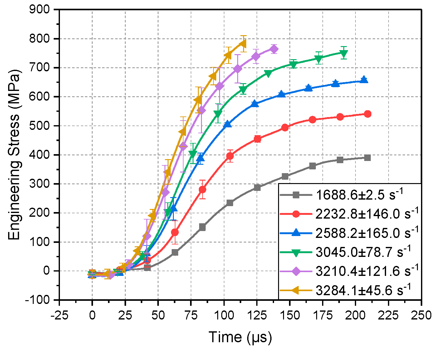
As shown in Figure 10, the maximum stress of the Φ9 × 4 specimens under different impact pressures increased with the increasing strain rate. If the specimen was not damaged completely, the maximum stress points usually happened around a certain time. If the specimen was damaged completely, the maximum stress points occurred earlier and earlier. Correspondingly, each zone in the damaged tests happened earlier and earlier under higher and higher strain rate.

(c) Effect of Strain Rate

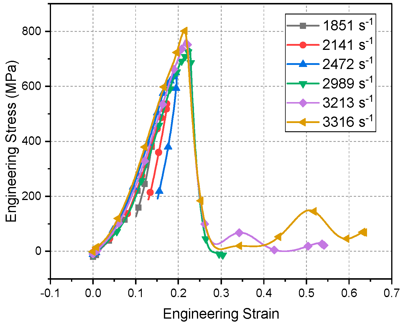
As Figure 11 shows, as the strain increased, it seems that the stress values under different strain rates increased along the same curve, where only the peak points were different.

If the specimen was not damaged completely, the peak stress refers to the maximum stress that the specimen could sustain under a certain strain rate. After the peak point, the specimen still had the ability to spring back, which could also be seen in the high-speed camera records. However, the spring-back curve was not the same as the loading curve. This was potentially because some fibers were squeezed out of the main body of the specimen and, thus, a certain degree of permanent damage was caused. Furthermore, the slopes of previous spring-back curves under different strain rates were similar [49], which means that the specimens retained similar properties.

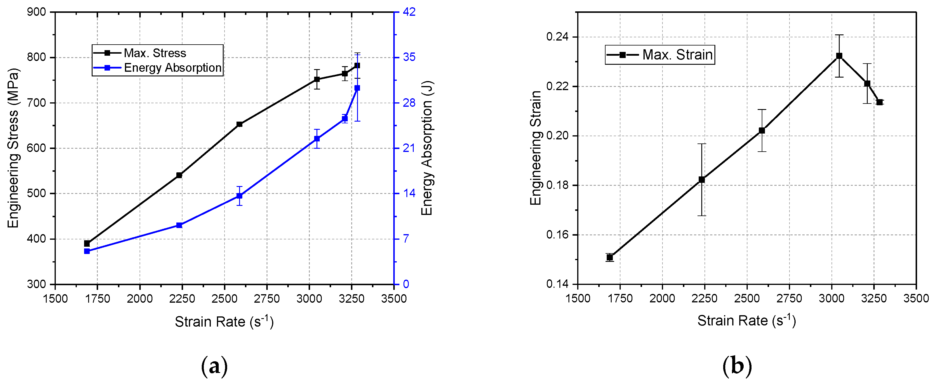
If the specimen was damaged completely, the peak stress refers to the fracture stress of the specimen. As shown in Figure 11 and Figure 12a after 2989 s⁻¹, the fracture stress also increased as the strain rate increased. Furthermore, as the strain rate increased, the soften zone of the stress–strain curve tended toward the linear period. Therefore, the slope of the stress–strain curve in the soften zone was higher and the fracture strain became smaller to some extent as the strain rate increased to 2989, 3213, and 3316 s⁻¹, as shown in Figure 11 and Figure 12b. This phenomenon also occurred in the non-damaged tests of specimens 8 x 8 x 4 when the strain rate became higher. To sum up, with the increasing strain rate, the maximum stress, fracture stress, and energy absorption also increased. In contrast, it seems that the maximum strain increased at first and then decreased when it became fracture strain.

As shown in Figure 13a–d for the Φ9 × 4 specimens under 0.2–1.2 MPa impact, as the strain rate increased, more fibers were squeezed out. Therefore, the little square at the center of the end face became more and more clear. As to the specimens under 3045.0018 ± 78.6690 s⁻¹ strain rate, some were non-damaged and some were completely damaged, which means that this strain rate represents the critical fracture value. As for the damaged specimens shown in Figure 13e,f, the main body was crushed into several relatively big blocks. The traces of the crushed parts indicate that they were damaged by inner shear stress.

As mentioned in Reference [21], compaction is the major failure mode in the out-of-plane direction, which represents the energy absorption mechanism. Similarly, as more compaction occurs, more fibers are squeezed out and more blocks are crushed; furthermore, with increasing strain rate, the energy absorption also increases. Shi also [21] found that the laminated angle has an effect on the dynamic energy absorption of composites at higher strain rates. Placing laminae in a well-proportioned manner on the projective plane effectively enhances the energy absorption load under transversal impact. The friction between fibers perhaps has a relationship with the placing angle and energy propagation, which needs deeper study in further work.

(d) Effect of Size

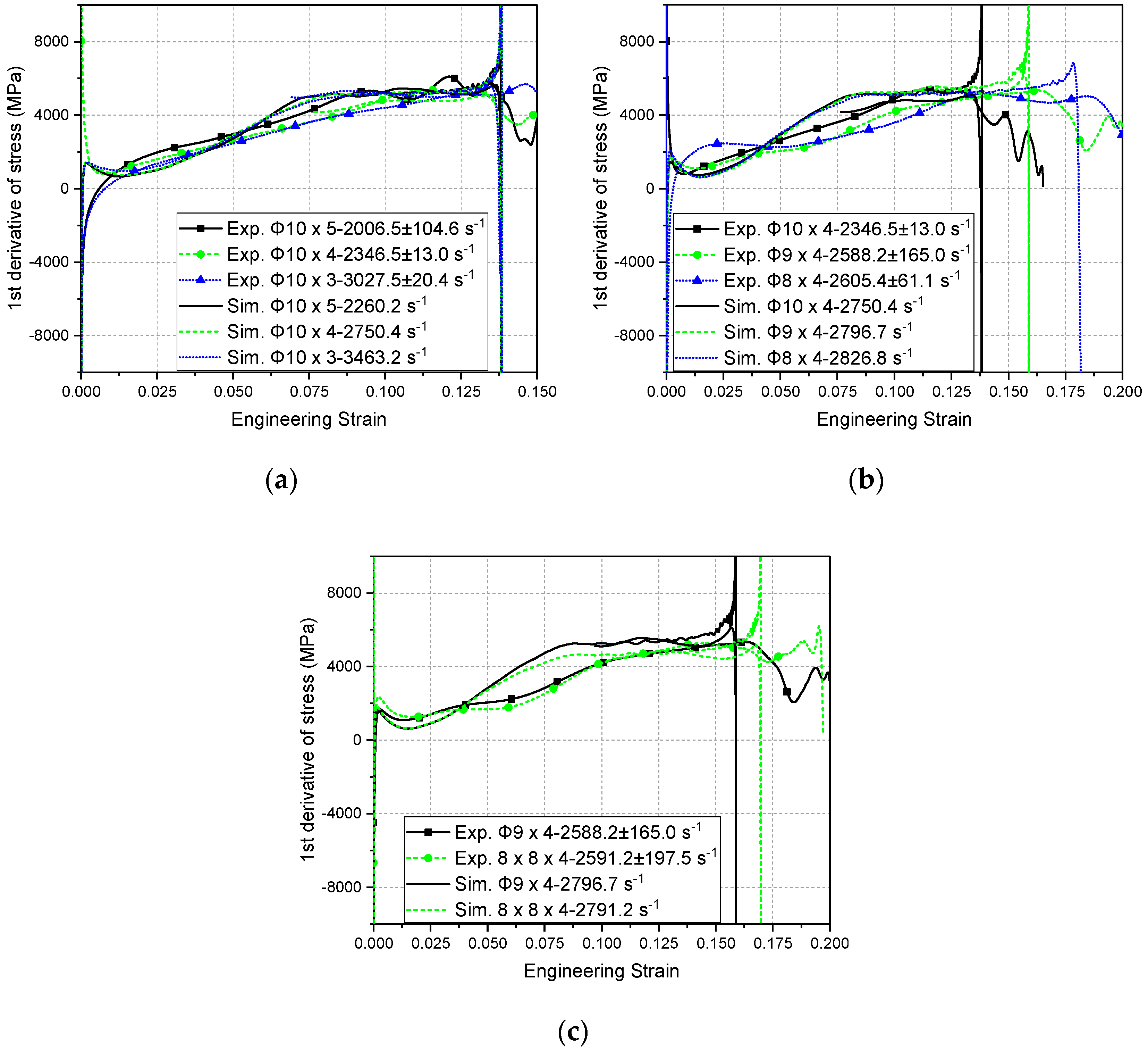
The non-linear and linear periods were mainly considered for size effects. For the influence of thickness, as shown in Figure 14a, if the thickness was different, the stress–strain relationships were obviously different. As shown in Figure 15a, with an increase in the thickness, the slope of the non-linear period became steeper and shorter. As shown in Figure 16b and

Table 2. The modulus of specimens of different sizes.

D-ls/L-W-ls	Area	Volume	Modulus	Mean	Absolute Difference	Relative Difference
	A	V	E	M	|E − M|	|E − M|/|M|
mm	(mm2)	(mm3)	(MPa)	(MPa)	(MPa)	(%)
Φ10 × 5	78.5398	392.6991	5237.9036	4986.0380 ± 283.5900	251.8655	5.0514
Φ10 × 4	78.5398	314.1593	5362.2738		376.2358	7.5458
Φ10 × 3	78.5398	235.6195	4641.9097		344.1284	6.9018
Φ9 × 4	63.6172	254.4690	4866.7752		119.2628	2.3919
Φ8 × 4	50.2655	201.0619	5063.2357		77.1977	1.5483
8 × 8 × 4	64.0000	256.0000	4744.1302		241.9078	4.8517

, the thickness seems to not significantly affect the modulus values of the linear period. Therefore, the thickness seems to affect the self-installation zone and the non-linear period, but it seems to not affect the linear period. Since the self-installation zone is inevitable for the SHPB apparatus, the thickness seems to mainly affect the non-linear period.

With regard to the influence of diameter/area, as shown in Figure 14b, the diameter or area seems to not significantly affect the stress–strain relationship. Considering Figure 15b and that the modulus of specimens with different diameter in Table 2 was similar, the diameter or area also seems to mainly influence the non-linear period. The influence of the area was not as obvious as the influence of the thickness. For the influence of shape, as shown in Figure 14c and Figure 15c, the stress–strain curves for different shapes were similar, and the slope of the cylindrical specimen was a little bit higher than that of the cuboid specimen in the non-linear period. In general, the thickness had the greatest influence on the non-linear period stress–strain curve, while the shape of the cross-section had the least influence.

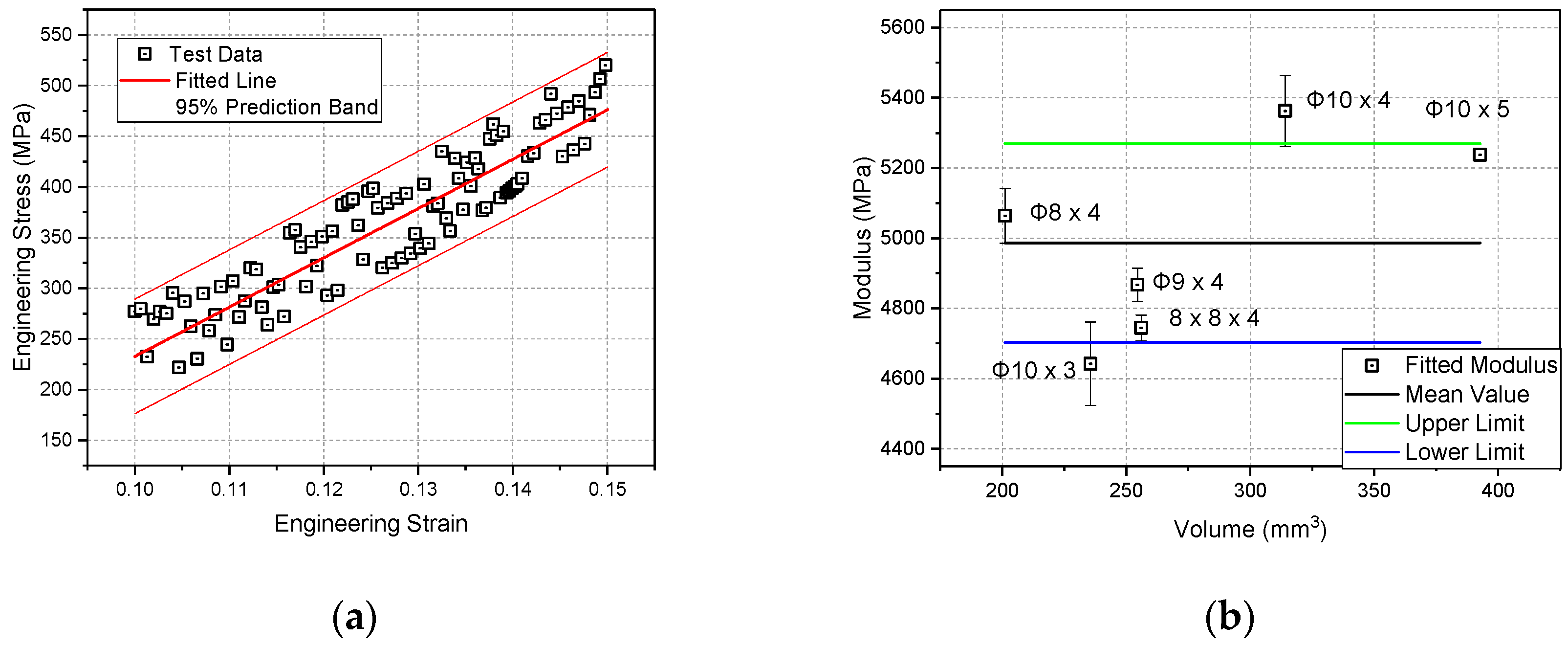
As shown in Figure 16a, the modulus of these specimens could be fitted using points in the linear period of the stress–strain curves. As shown in Table 2 and Figure 16b, the modulus values did not show a strong relationship with the thickness, area, volume, or shape of the specimen. The maximum relative error when comparing the mean values was 7.5458%.

3.1.3. Comparison of Quasi-Static and Dynamic Behavior

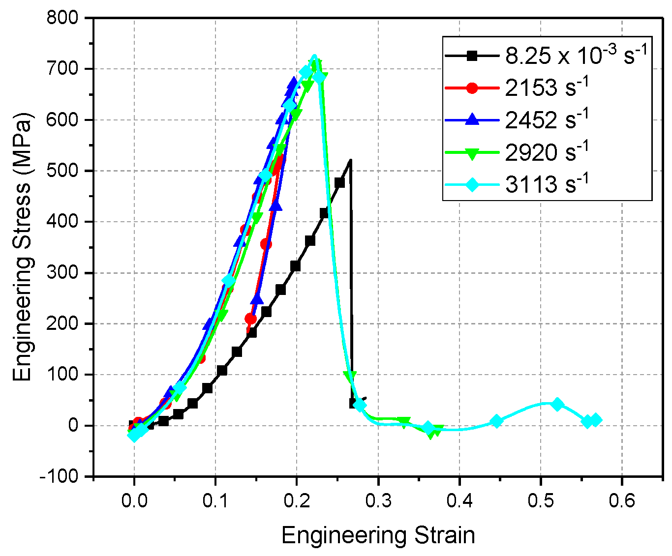
To avoid uncertainties related to size effects [17], the results of specimens of the same size under quasi-static and dynamic tests are compared in Figure 17. With regard to the evolution features, the dynamic stress–strain curves were different from the quasi-static stress–strain curve. During quasi-static loading, the stress increased as the strain increased, and finally the specimen failed at the fracture point. On the other hand, during dynamic loading, there were two different features after the peak point. One feature is that, when the strain rate was 2153 or 2452 s⁻¹, there was a spring-back and the slope of the spring-back curve was similar. Another feature is that higher strain rates led to the specimens being damaged completely with the spring-back phenomenon disappearing.

With regard to the damaged features, the dynamic features were different from the quasi-static features. It can be seen from Figure 17 that the stress–strain curve of the quasi-static test dropped like a cliff, while the stress–strain curve of the dynamic test dropped relatively slowly. For the quasi-static test, this was possibly because the loading speed was slow, and the duration from the fracture moment to the specimen becoming compact again was long. In this duration, the specimen could not hold any loading; thus, the stress was nearly 0. In contrast, the loading speed of the dynamic test was fast, and the duration from the fracture moment to the specimen becoming compact again was short. Thus, the specimen could hold loading to some extent during the fracture process. Therefore, the dynamic stress–strain curve dropped relatively slowly. Furthermore, as seen in a previous study [36], a second loading curve was also observed in the damaged test, which can be seen in Figure 11 for the Φ9 × 4 specimens.

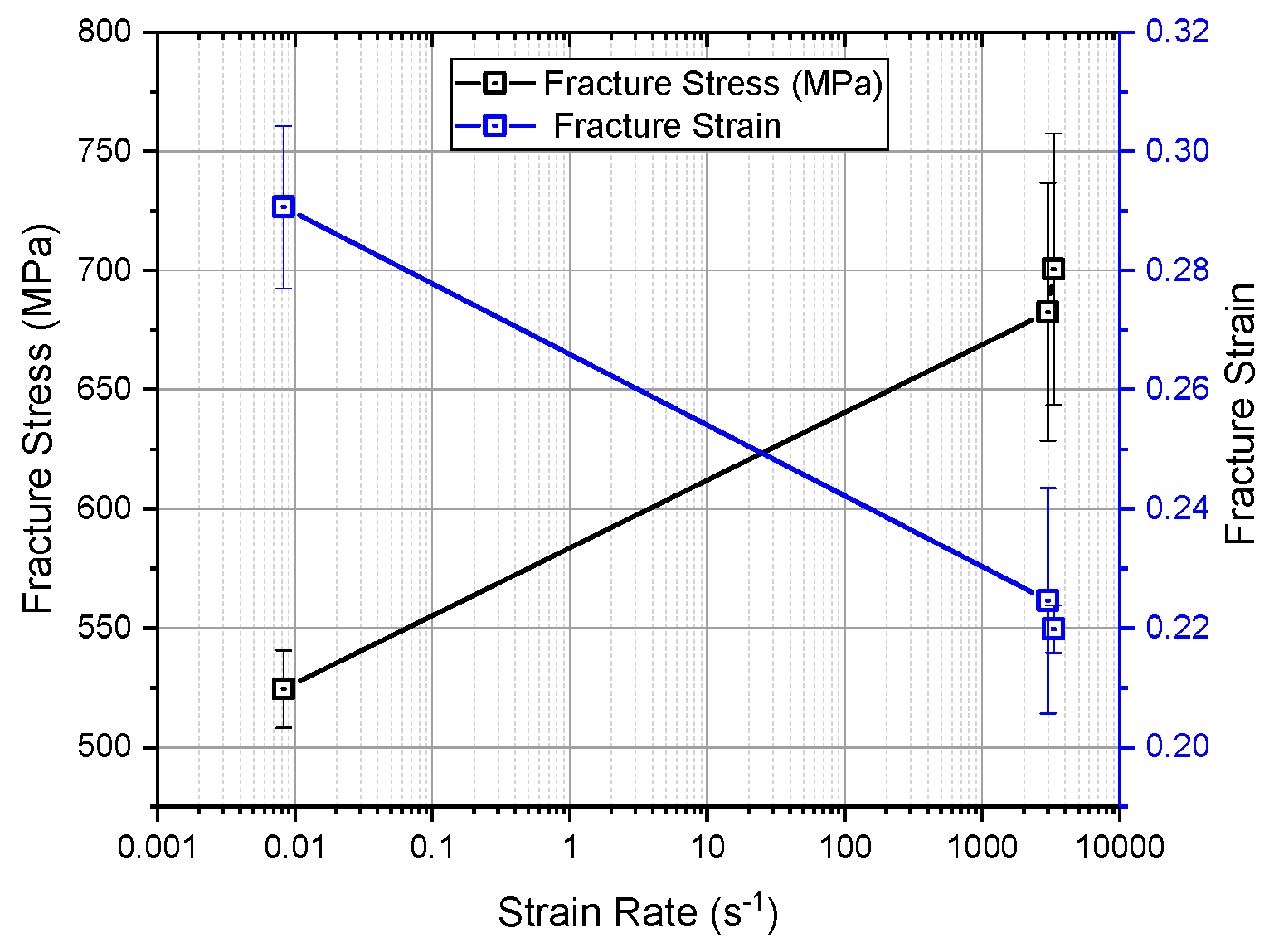
As shown in Figure 18, the fracture stress under high-strain-rate loading was higher than the fracture stress under quasi-static loading. Moreover, the fracture stress under high-strain-rate loading kept increasing as the strain rate increased, which can also be seen in Figure 11b. In contrast, the fracture strain under high-strain-rate loading was lower than the fracture strain under quasi-static loading. The quantitative results are provided in

Table 3. The fracture stress and strain in out-of-plane direction under increasing strain rates.

Strain Rate	Fracture Stress	Fracture Strain
s−1	MPa
8.307 × 103 ± 5.4029 × 10−5	524.3487 ± 16.2298	2.906 × 10−1 ± 1.366 × 10−2
3000.9948 ± 116.4061	682.6499 ± 54.0770	2.246 × 10−1 ± 1.892 × 10−2
3307.6690 ± 182.6697	700.5194 ± 56.9639	2.198 × 10−1 ± 3.990 × 10−3

.

3.2. In-Plane Test

3.2.1. Quasi-Static Compression

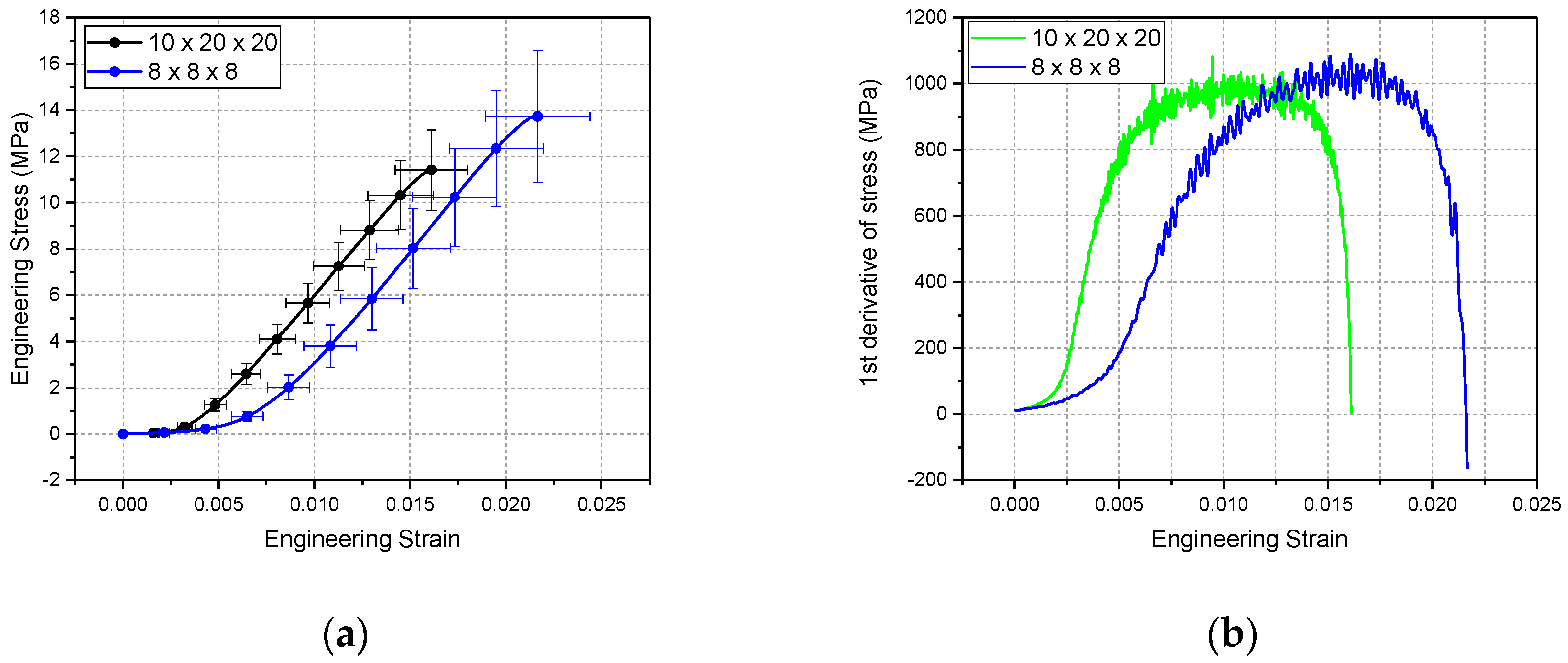
Two sizes of specimens were studied. The loading speed was 2 mm/min; thus, the strain rate for 10 × 20 × 20 specimens was 1.67 × 10⁻³ ± 3.7550 × 10⁻⁶, and the strain rate for the 8 × 8 × 8 specimen was 4.18 × 10⁻³ ± 3.0301 × 10⁻⁷. As shown in Figure 19a, the fracture stress and strain of the bigger specimens were lower than those of the smaller specimens. As shown in Figure 19b, it is obvious that there were three phases during the loading. In the first phase, maybe because the pores among the specimen were compressed, the stress–strain curve was non-linear and the slope increased rapidly. In the second phase, the stress–strain curve could be seen as linear. The modulus values of these two sizes of specimens were similar. In the third phase, the stress–strain curve seems to present material softening before failure.

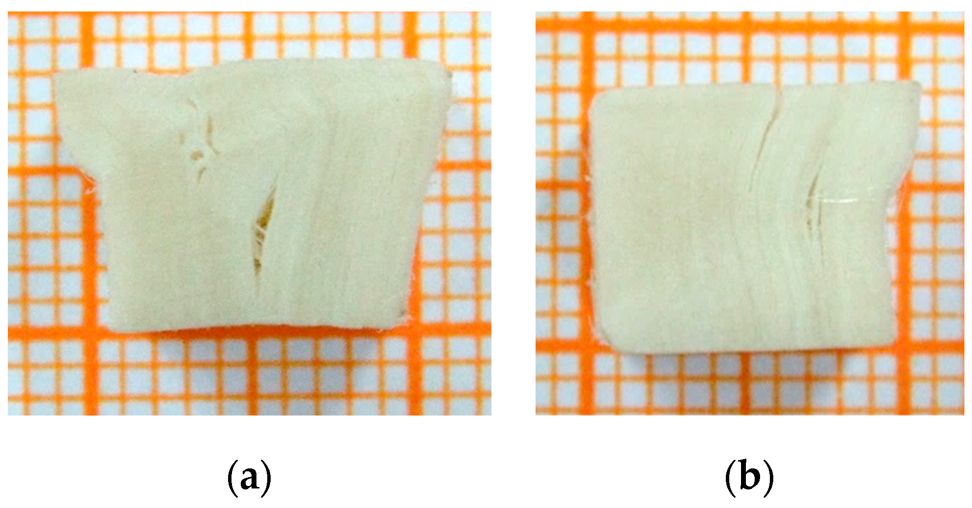
As shown in Figure 20 and Figure 21, there were kink bands [18] along with fibers in both small and big specimens. The kink bands showed two kinds of typical features. One feature is shown in Figure 20a and Figure 21a, where one major kink band ran through the specimen and delamination began to generate at the upper or lower side. The other feature is shown in Figure 20b and Figure 21b, where two kink bands in an X shape ran through the specimen and delamination began to generate in the middle part of the main body. In addition, by comparing Figure 20 and Figure 21, for the smaller specimen, the whole specimen was involved in the fracture, while, for the bigger specimen, only the local part was involved in the fracture.

3.2.2. Dynamic Compression

(a) Mechanical Behavior

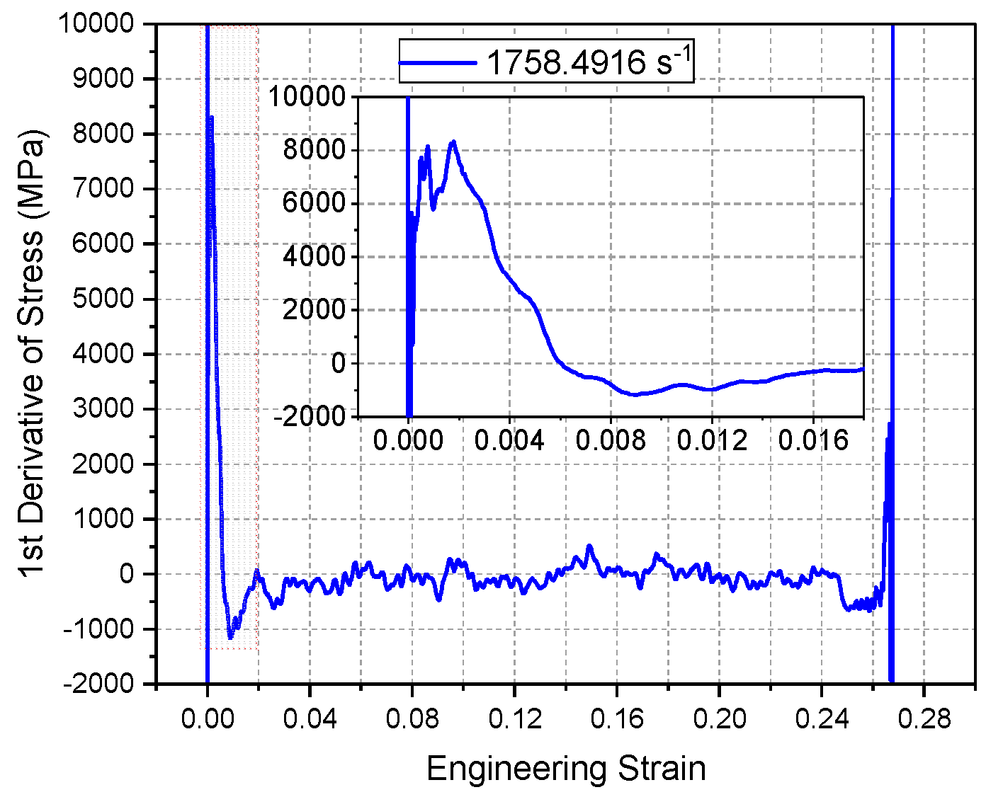
The whole first-derivative course of the specimen under 0.2 MPa loading is shown in Figure 22. After a fast increase, the first derivative fluctuated around a certain constant. This certain period of the stress–strain curve can be seen as linear. The first derivative then dropped slowly and finally fluctuated around zero.

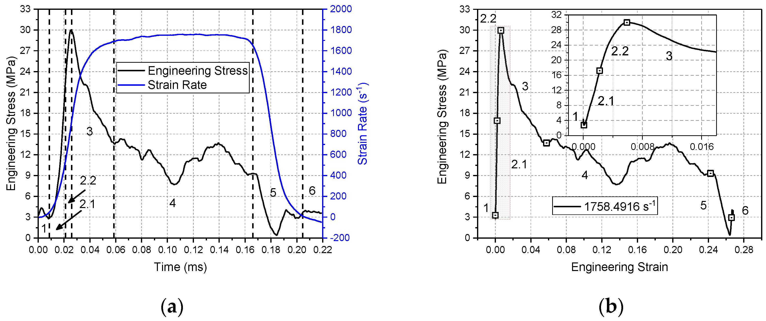
According to the analysis, for the loading evolution of the 8 × 8 × 8 specimen under 0.2 MPa loading, shown in Figure 23, the stress–strain curve could be separated into six zones.

Zone 1: This period is called the self-installation zone. The strain rate increased slowly, and the stress fluctuated near a very small value. This is because the parallelism of the specimen faces in contact with the bars was not 100% guaranteed. This period was very short.

Zone 2: This period is called the under-loading zone. The strain rate increased rapidly, and the stress also increased quickly to a maximum value. As shown in Figure 23b, this zone could be divided into a linear period and non-linear period. This zone represents the main dynamic behavior of the specimen under in-plane loading.

Zone 3: This period is called the fracture zone. The strain rate kept increasing, while the stress decreased after the fracture point. This shows that the specimen’s holding ability did not vanish suddenly but gradually.

Zone 4: This period is called the distorted zone. The strain rate was almost constant in this zone. The fluctuation of stress was big. After a drop, the stress increased to a second peak followed by another drop. This was possibly because the damaged specimen was squeezed, thereby becoming more compact, but it was simultaneously folded and distorted. As a result, the compact specimen could hold the loading to some extent. The distorted structure resulted in the stress fluctuating very unsteadily.

Zone 5: This period is called the unloading zone. The strain rate decreased in this zone. The stress also decreased relatively rapidly.

Zone 6: This period is called the ending zone. The strain rate became zero and the loading ended. Finally, the stress fluctuated around a small value.

(b) Damage Kinetics

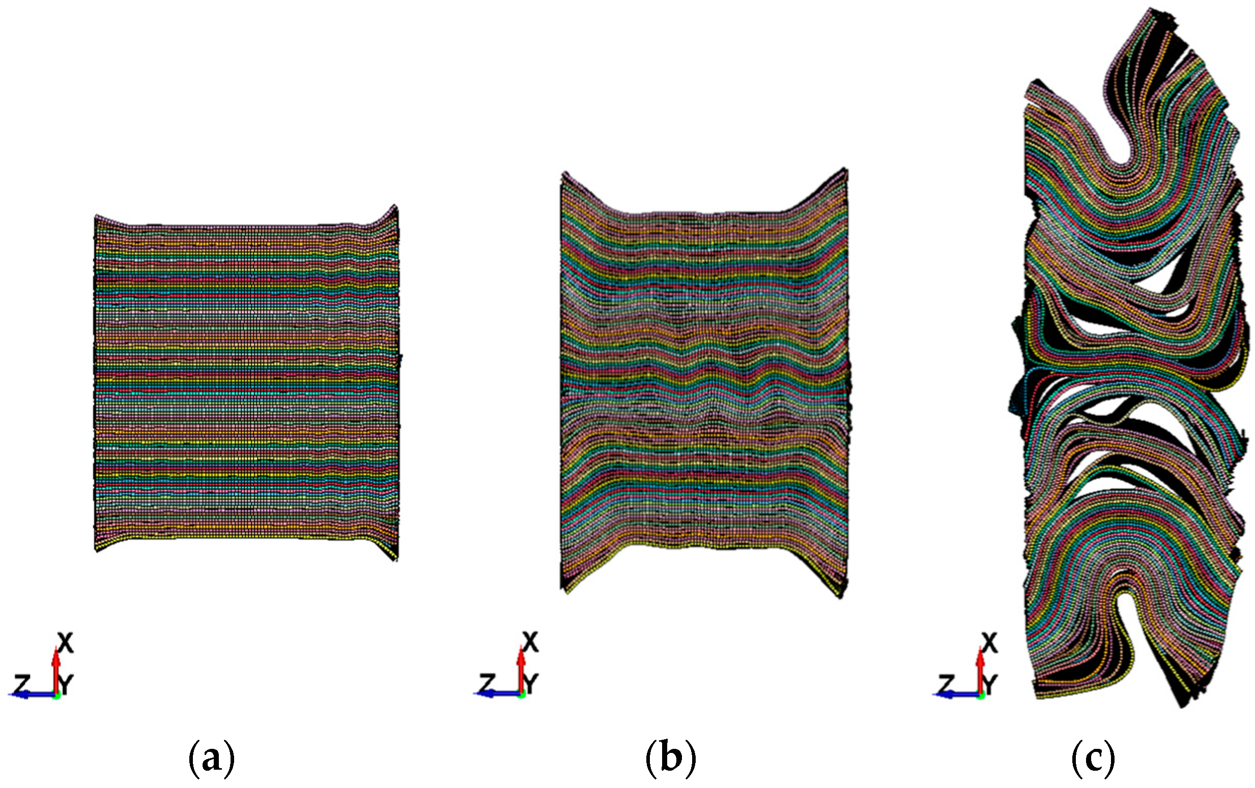
As showed in the circles of Figure 24b in comparison with Figure 24a,c for the 8 × 8 × 8 specimen under 0.2 MPa loading, when the corner of the specimen in contact with the input bar was squeezed vertically, the specimen failed at this moment. This moment corresponds to the fracture point on the stress–strain curve shown in Figure 23. At first, the fracture happened at the side of the specimen near the input bar. Then, as more layers were squeezed apart vertically, the stress fell gradually from 23.69 to 52.12 μs. In this period, as the input bar moved forward, the fracture persisted and the layers on the contact surface were gradually squeezed vertically. The remainder of the specimen could still hold loading to some extent, as shown in Figure 24c. Finally, the remainder of the specimen was shortened, preventing it from maintaining contact. After this, as the input bar kept moving forward, the whole body of the specimen was squeezed, distorting it as shown in Figure 24d. In addition, because the morphology of the layers squeezed vertically was similar, it could be concluded that the parallel degree of the two ends near the input and output bars was good. Moreover, the fracture pattern under high-strain-rate loading was a kind of delamination similar to that presented in References [18,50,51], as opposed to the kink bands seen in quasi-static loading [18].

(c) Effect of Strain Rate

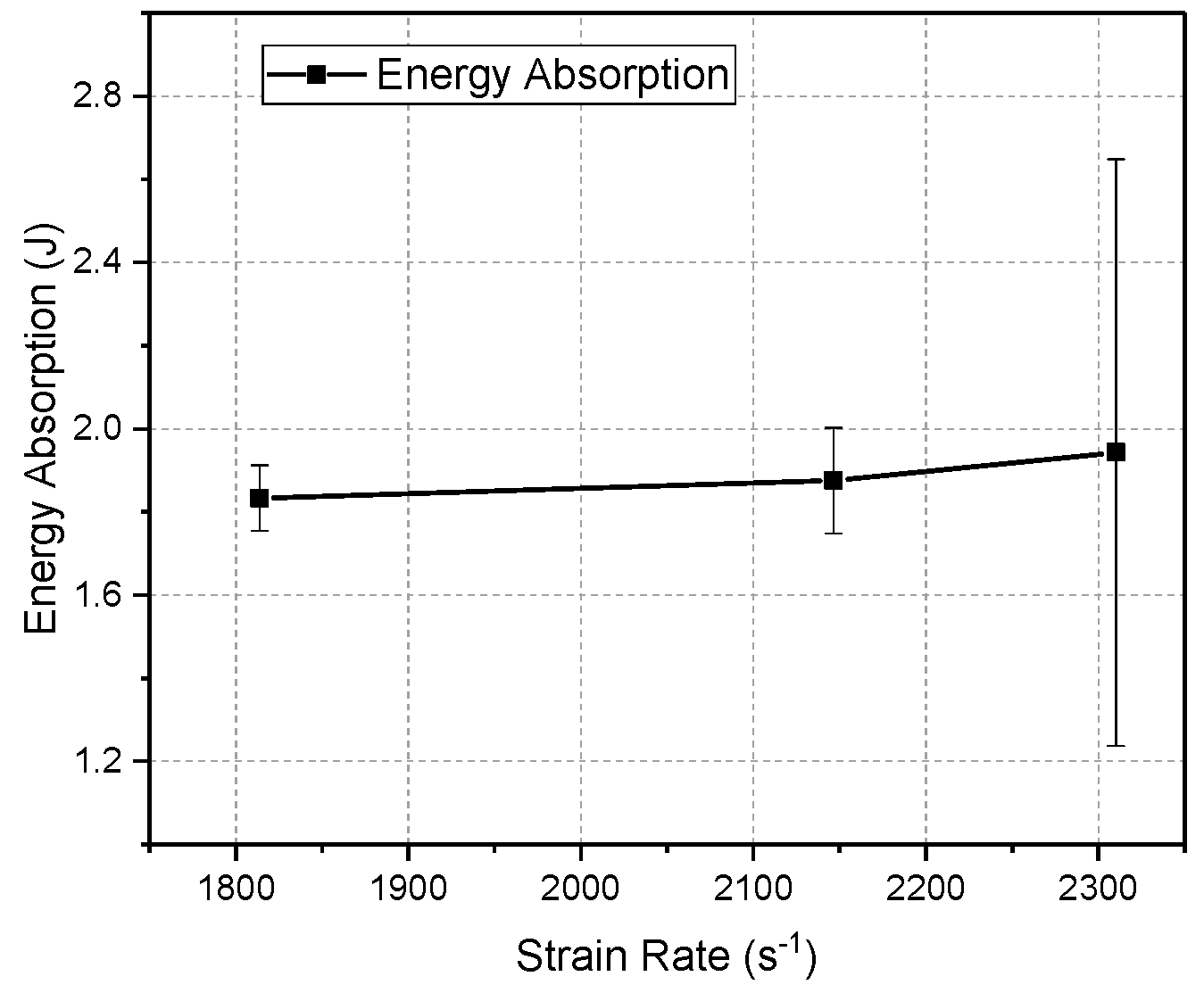
As shown in Figure 25, with the strain rate increasing, the energy absorption increased as well, albeit slowly. As shown in Figure 24 and Figure 26, some parts were squeezed out of the specimen’s main body, while some parts remained. The stress–strain curves of 8 × 8 × 8 specimens are shown in Figure 27b. The fracture stress and strain also increased with increasing strain rate. The modulus decreased slightly with increasing strain rate, as shown in Figure 28b.

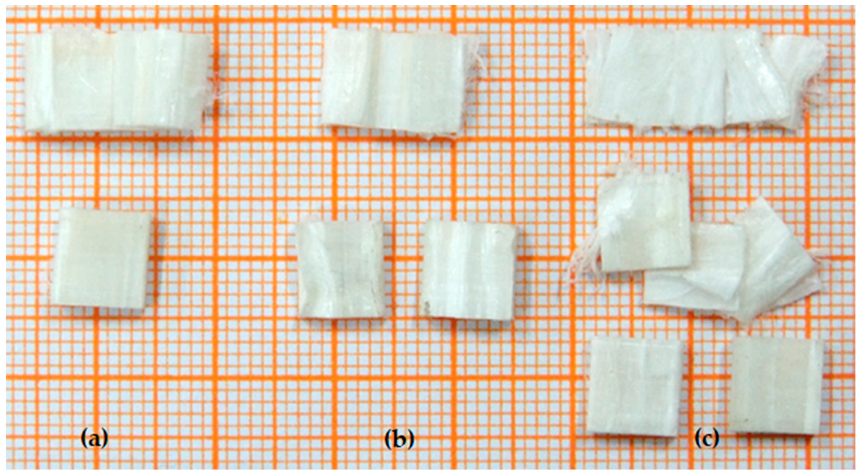
As shown in Figure 26, a higher strain rate resulted in the remaining parts being more compact due to squeezing. In addition, as the strain rate increased, more pieces were squeezed out of the specimens, and the pieces that were squeezed out were more folded.

(d) Effect of Size

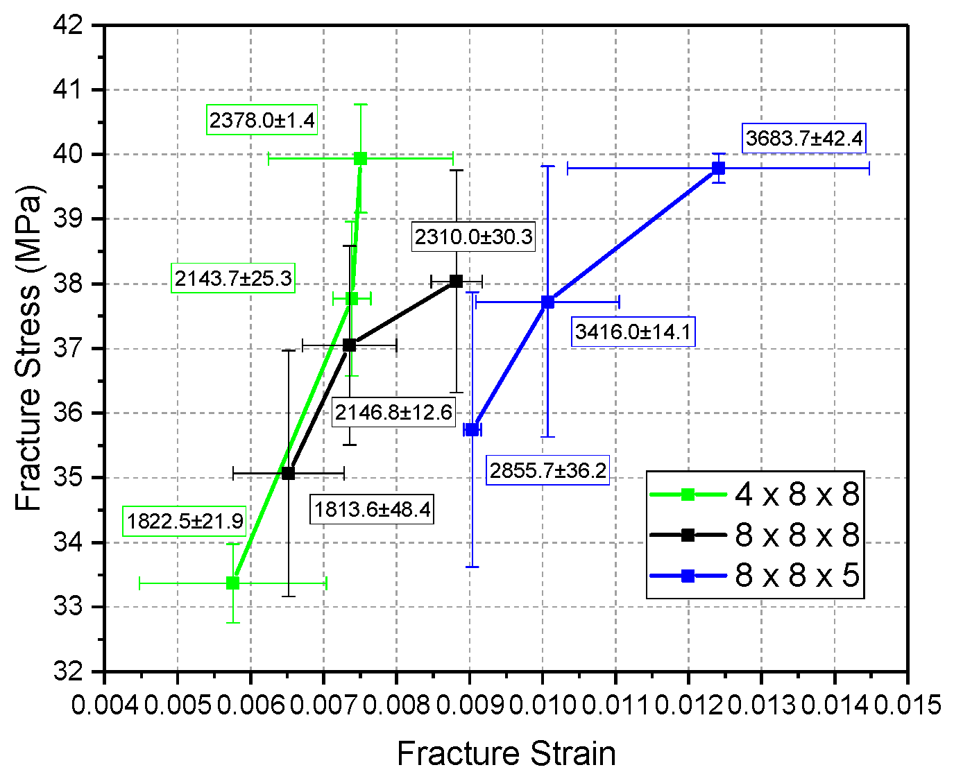
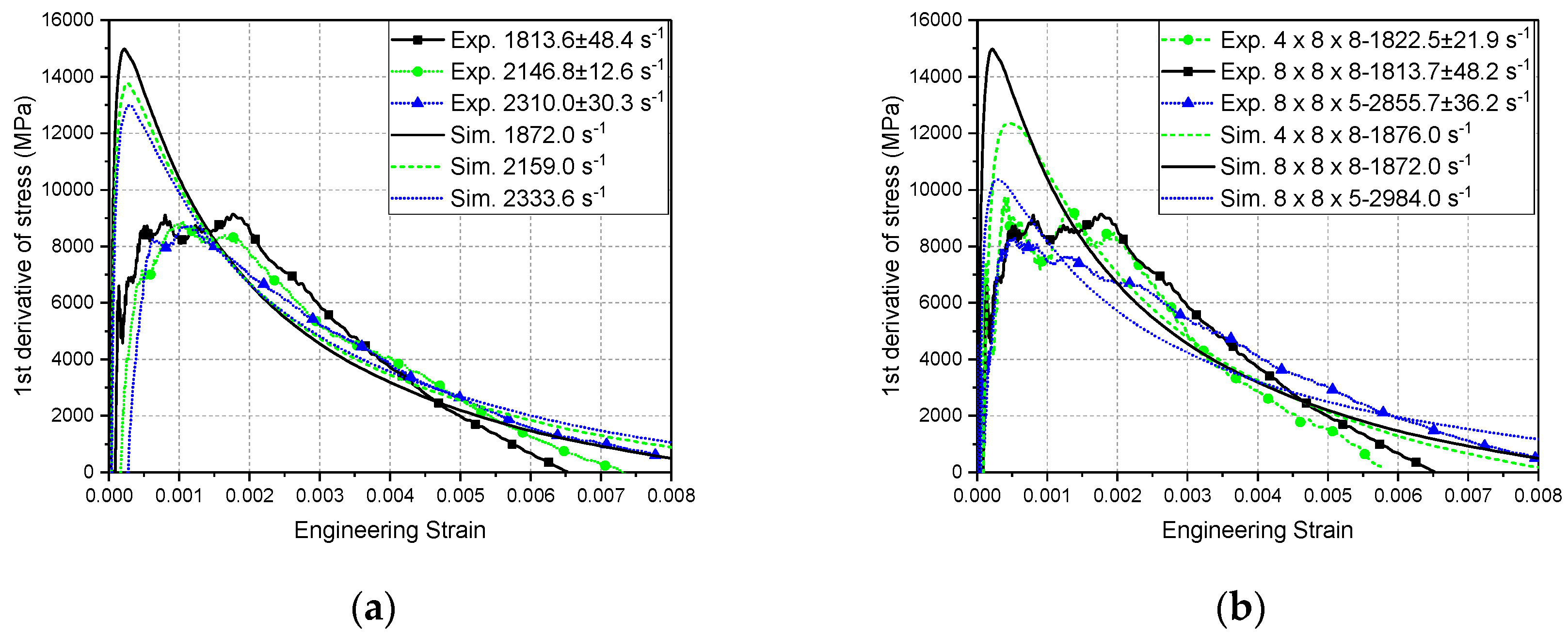
Specimens of different sizes showed similar strain rate effects. Firstly, as shown in Figure 27, with the increase in strain rate, the corresponding stress–strain curves of specimens of the same size were not significantly different. The only difference was that the position of the fracture point kept moving forward. As shown in Figure 30, the same trend can be found, whereby an increase in strain rate led to both fracture stress and strain increasing for all specimens with different sizes. Secondly, by taking the first derivative of the stress–strain curves shown in Figure 28, there was a specific period in which the first derivative oscillated steadily for specimens of all sizes. It could be inferred that this period of the stress–strain curve could be regarded as linear. The slope of this period could be seen as the modulus. Thirdly, the modulus of these three specimens all decreased to some extent with the increasing strain rate, in which the modulus of the 8 × 8 × 8 specimens decreased relatively slightly, while the modulus of the 8 × 8 × 5 specimens decreased relatively clearly. Since the reduction was not much, the modulus could be considered as a constant value, as shown in

Table 4. The modulus of specimens of different sizes.

L-W-ls	Area	Volume	Modulus	Standard Deviation
mm	mm2	mm3	MPa	MPa
4 × 8 × 8	32	256	8002.1508	83.5371
8 × 8 × 8	64	512	8395.8743	36.6529
8 × 8 × 5	64	320	6120.0996	106.9114

.

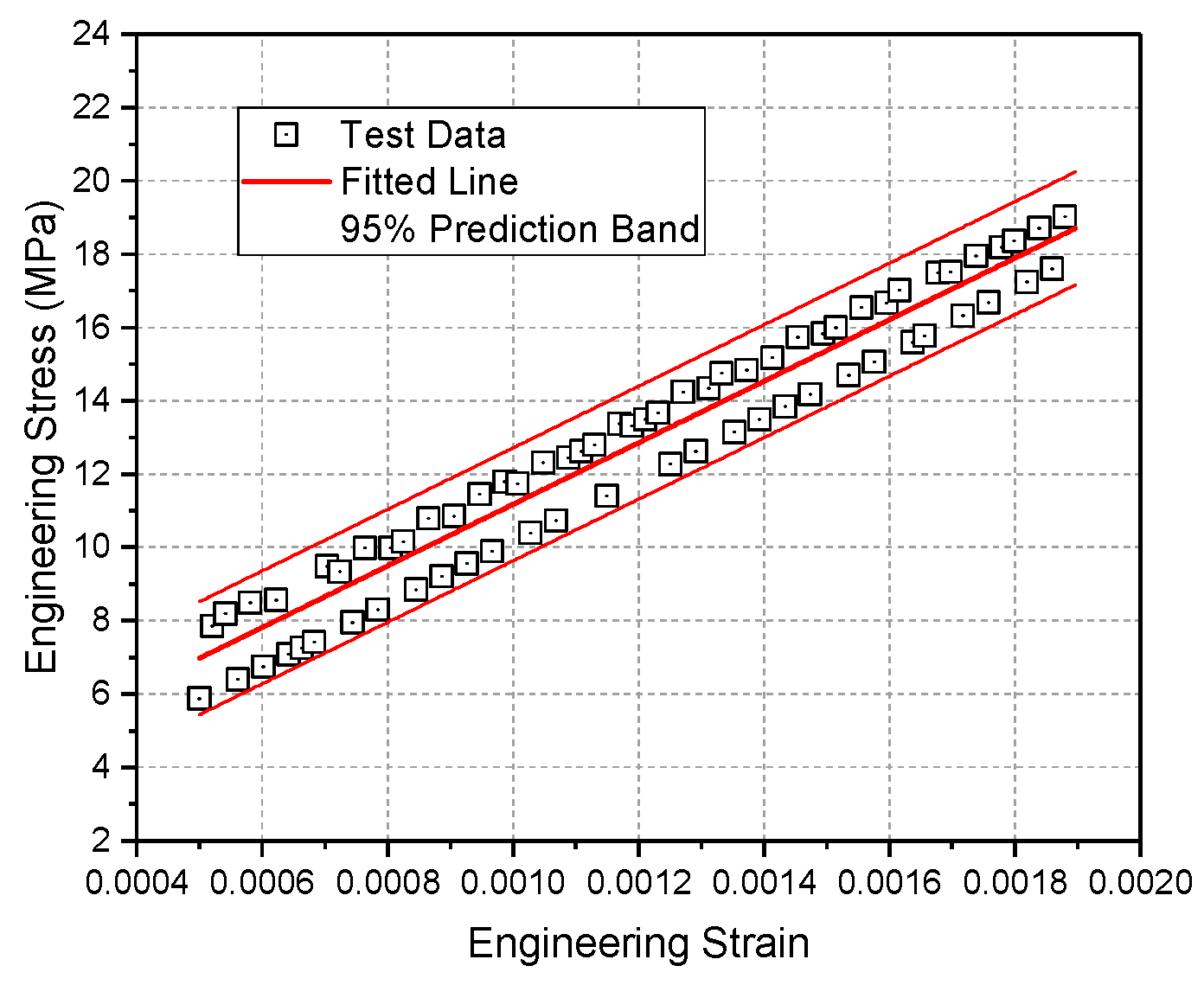
According to Figure 22 and Figure 28, the linear modulus of the 8 × 8 × 8 specimens could be fitted using the points in the stable oscillation linear period of the stress–strain curves, as shown in Figure 29. The modulus of the specimens of different sizes is presented in Table 4. It seems that the influence of thickness was greater than the influence of area on the modulus of specimens.

There were also some differences between specimens of different sizes. Firstly, as shown in Figure 27, the stress–strain curves of the 8 × 8 × 8 specimens were more stable, and the tendency of the stress–strain curves increasing with the strain rate was more regular than for the curves of 4 × 8 × 8 specimens and 8 × 8 × 5 specimens. As shown in Figure 28b, the values of the first derivative in this period for the 8 × 8 × 8 specimens under different strain rates were more similar and fluctuated less. This is maybe because the area and thickness of the 8 × 8 × 8 specimens were bigger and, thus, the properties inside the specimens were more uniform and consistent. Secondly, as shown in Figure 30, the fracture points of the 4 × 8 × 8 specimens were closer to the fracture points of the 8 × 8 × 8 specimens, while the fracture points of the 8 × 8 × 5 specimens were obviously further away. This is because the modulus values of the 8 × 8 × 8 and 4 × 8 × 8 specimens were more similar than that of the 8 × 8 × 5 specimens, as shown in Table 4. Thirdly, it seems that the size of the specimens mainly influenced the modulus but did not obviously influence the fracture stress.

3.2.3. Comparison of Quasi-Static and Dynamic Behavior

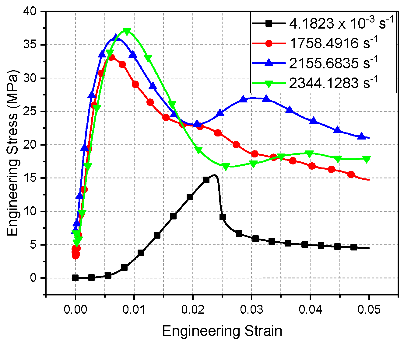
To avoid uncertainties related to size effects [17], the results of specimens of the same size under quasi-static and dynamic tests are compared in Figure 31. The dynamic behavior was different from the quasi-static behavior. One different feature is that the stress–strain relationship of the quasi-static loading was firstly non-linear and then linear, while the stress–strain relationship of the dynamic loading seems to be firstly linear and then non-linear. Another different feature is that, after fracture, the stress–strain curve showed a sudden drop in the quasi-static loading, while the stress–strain curve dropped gradually in the dynamic loading. There were also some similar features between dynamic and quasi-static behavior. During both quasi-static and dynamic loading, the stress increased as the strain increased, and finally the specimen failed at the fracture point. In addition, the specimen could still hold the loading to some extent after fracture in both quasi-static and dynamic loading [28].

With regard to the fracture stress shown in Figure 32a, the dynamic fracture stress was higher than the quasi-static fracture stress. The dynamic fracture stress kept increasing as the strain rate increased. With regard to the fracture strain shown in Figure 32a, the dynamic fracture strain was lower than the quasi-static fracture strain. The dynamic fracture strain rate increased with the increasing strain rate. With regard to the modulus shown in Figure 32b, the modulus under dynamic loading was higher than the modulus under quasi-static loading. The dynamic modulus decreased slightly with the increasing strain rate.

Table 5. The fracture stress, strain, and modulus in the in-plane direction under increasing strain rates.

Strain Rate	Modulus	Fracture Stress	Fracture Strain
s−1	MPa	MPa
4.180 × 10−3 ± 3.030 × 10−7	985.73404 ± 3.5528	13.7369 ± 2.8497	2.167 × 10−2 ± 2.740 × 10−3
1813.5829 ± 48.4181	8553.5254 ± 85.4232	35.0658 ± 1.9018	6.520 × 10−3 ± 7.650 × 10−4
2146.7858 ± 12.5833	8391.0523 ± 398.3287	37.0466 ± 1.5355	7.360 × 10−3 ± 6.435 × 10−4
2309.9629 ± 30.2695	8351.9092 ± 417.6605	38.0406 ± 1.7206	8.820 × 10−3 ± 3.495 × 10−4

shows the quantitative results of the 8 × 8 × 8 specimens.

4. Numerical Results and Discussion

Finite element simulations of the high-strain-rate compression tests were performed by LS-DYNA 971. As mentioned before, the length of the steel striker bar was 0.5 m, while the length of the aluminum striker bar was 0.4 m. The numbers of elements used in these striker bars were 60,000 and 48,000, respectively. The length of both the input and the output bars was 1.5 m. The number of elements used in these bars was 180,000. Their diameters were all 14.5 mm. The number of elements on the cross-section was 300 for all these bars. The *MAT_ELASTIC material model was used for all the bars. The values of density, Young modulus, and Poisson’s ratio for the steel and aluminum bars were 7.85 × 10³ kg/m³, 206 GPa, 0.27 and 2.8 × 10³ kg/m³, 72 GPa, 0.32, respectively. The eroding surface-to-surface contact was defined between the specimen and input/output bar. The eroding single-surface contact was defined between the composite sub-laminates [28,52]. The “soft” contact option type 2 was utilized for the eroding contact [52]. The automatic surface-to-surface contact was defined between the striker bar and input bar. An initial velocity was defined for the striker bar according to the impact velocity measured in the experiments under a certain impact pressure [17].

The cohesive element was applied to simulate the cohesive failure using the *MAT_COHESIVE_MIXED_MODE material model [24,26,52]. The traction–separation relationship is shown in Figure 33. EN and ET are the initial slopes of the stress–displacement relationship before separation in the normal and tangential directions, with units of stress/length. T and S are the peak stress in the normal and tangential directions. ΔN and ΔS are the total displacement at complete separation in the normal and tangential directions. In addition, GIC and GIIC are the energy release rates for the normal and tangential directions, with units of stress ∙ length. The value of EN/ET was chosen to be sufficiently large, so as to essentially prevent separation before the unloading [24].

4.1. Out-of-Plane Simulation

4.1.1. Numerical Model

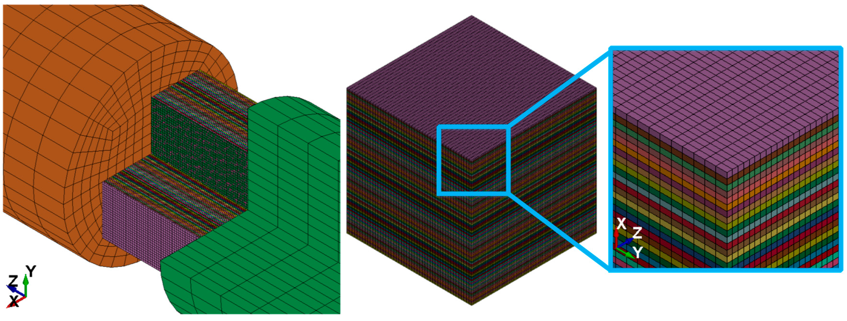
The FE model of the bars and specimen is shown in Figure 34. The size of the specimen was 8 × 8 × 4 mm. The loading direction and out-of-plane direction were both parallel to the z-axis direction. The out-of-plane direction was the x-axis direction. The specimen was discretized into 20 sub-laminates to form multiple layers through the thickness [4,23]. Each sub-laminate contained two layers of elements, as shown in detail in Figure 34, which represents one [0°/90°/0°/90°] stack. A layer of cohesive element between sub-laminates was applied [52].

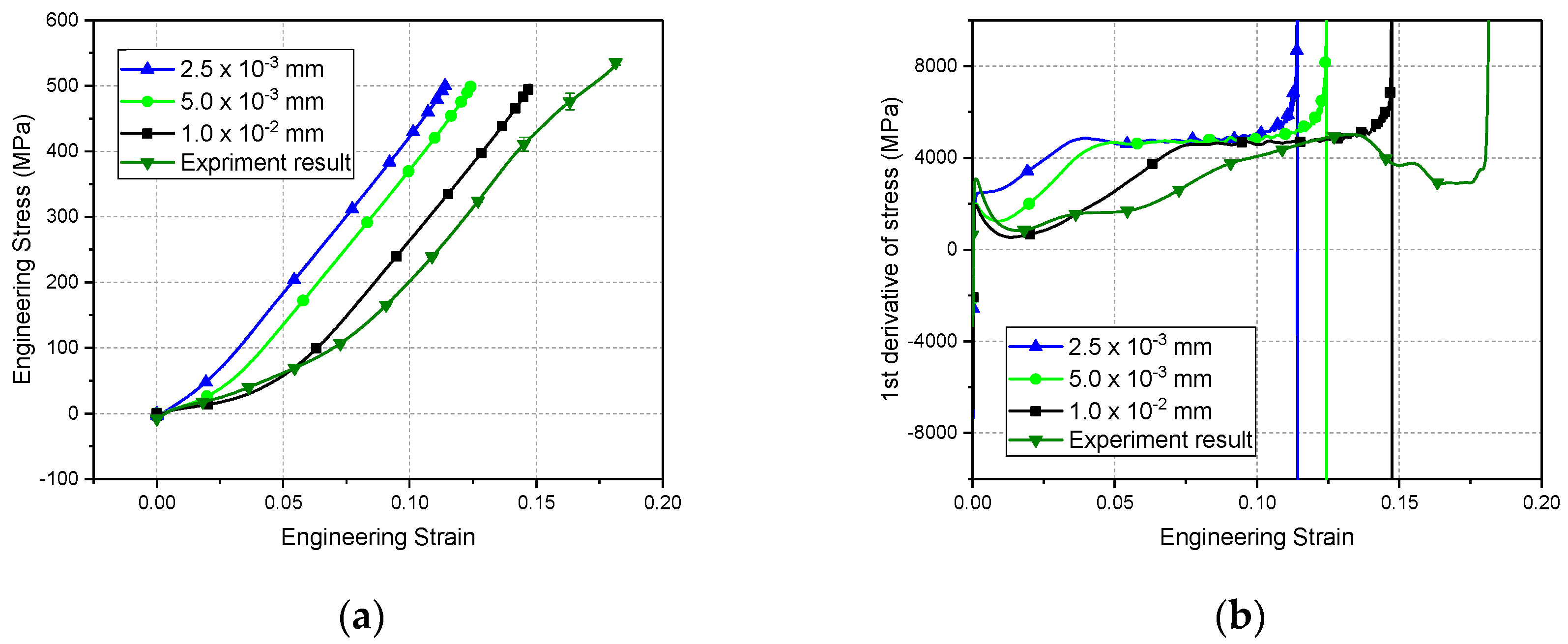
In addition, according to Reference [23], a small gap between two neighbor sub-laminates could solve the over-penetration of elements to some extent. Therefore, a small thickness was defined for the cohesive element. As shown in Figure 35, the influence of different gap thicknesses under 0.4 MPa loading was determined. A larger gap thickness resulted in the slope of the non-linear period of the simulation result being closer to the experimental result. The slope of the linear period and the maximum stress did not vary with the gap thickness. Therefore, a gap thickness of 1.0 × 10⁻² mm was applied. Thus, the sum of all gaps was 0.19 mm, which is small (<5%) compared to the total thickness of the specimen; it could then be considered to have a negligible effect on the ballistic performance [23]. This result also indicates that the non-linear period was mainly caused by the gap between sub-laminates. The element size of the sub-laminate was 0.2/0.2/0.1 mm. The total element amount of the specimen was 94,000, in which the element amount of sub-laminates was 64,000 and the element amount of cohesive element was 30,400.

The sub-laminate was studied using the *MAT_COMPOSITE_FAILURE_SOLID_MODEL. Since the composite plate used here and the plate used in Reference [4] were taken from the same factory, the material parameters shown in

Table 6. Material model properties of UHMWPE composite used in the out-of-plane direction [4].

Parameter: Value	Parameter: Value
Density, ρ (kg/m3) [4]: 0.97	AOPT, MACF [4]: 3.0, 1.0
Young’s modulus, Ea, Eb, Ec (GPa): 70, 70, 8	Tensile strengths, XT, YT, ZT (GPa) [4]: 3, 3, 3
Poisson’s ratio, νba, νca, νcb [4]: 0.006, 0.06, 0.06	Compressive strengths, XC, YC, ZC (GPa) [4]: 2, 2, 2
Shear modulus, Gab, Gbc, Gca (GPa) [4]: 4.6, 5, 5	Shear strengths, Sba, Sca, Scb (MPa): 600, 600, 600

were derived from Reference [4]. The AOPT is Material axes option and the MACF is Material axes change flag for brick elements. The cohesive material parameters mostly derived from Reference [24] are shown in

Table 7. Material model properties of cohesive element used in the out-of-plane direction [14,24].

Parameter: Value	Parameter: Value
Normal strength, T, (MPa) [14]: 1.0	Shear strength, S (MPa) [24]: 1.6
Normal stiffness, EN (MPa/mm): 400.0	Shear stiffness, ET (MPa/mm) [24]: 689.0
Energy release rate for mode I, GIC, (MPa·mm): 0.05	Energy release rate for mode II, GIIC, (MPa·mm) [24]: 0.1016

, in which T was cited from Reference [14]. G_IC and G_IIC are equal to T*E_N/2 and S*E_T/2, respectively, as shown in Figure 33. According to the current slope of the linear period of the dynamic stress–strain curve, E_a/E_b and Ec were estimated as ranging from 93 GPa and 11.5 GPa to 70 GPa and 8 GPa [25]. Because the shear failure happened during loading, S_ba, S_ca, and S_cb were estimated as ranging from 500 MPa in Reference [4] to 600 MPa, thereby better fitting the current maximum stress and its increasing trend. E_N and E_T were estimated according to the notion that, if they are higher, the slopes of the non-linear and linear periods would also be higher. The dynamic tests could allow obtaining more suitable material parameters for the current specimen applied in the numerical model. The material properties and failure criterion of the numerical model have a comprehensive relationship with both sub-laminates and cohesive elements. Therefore, in future work, it will be essential to separately study the dynamic properties of the fiber and dynamic cohesive properties of the matrix, and then study the integrated criterion.

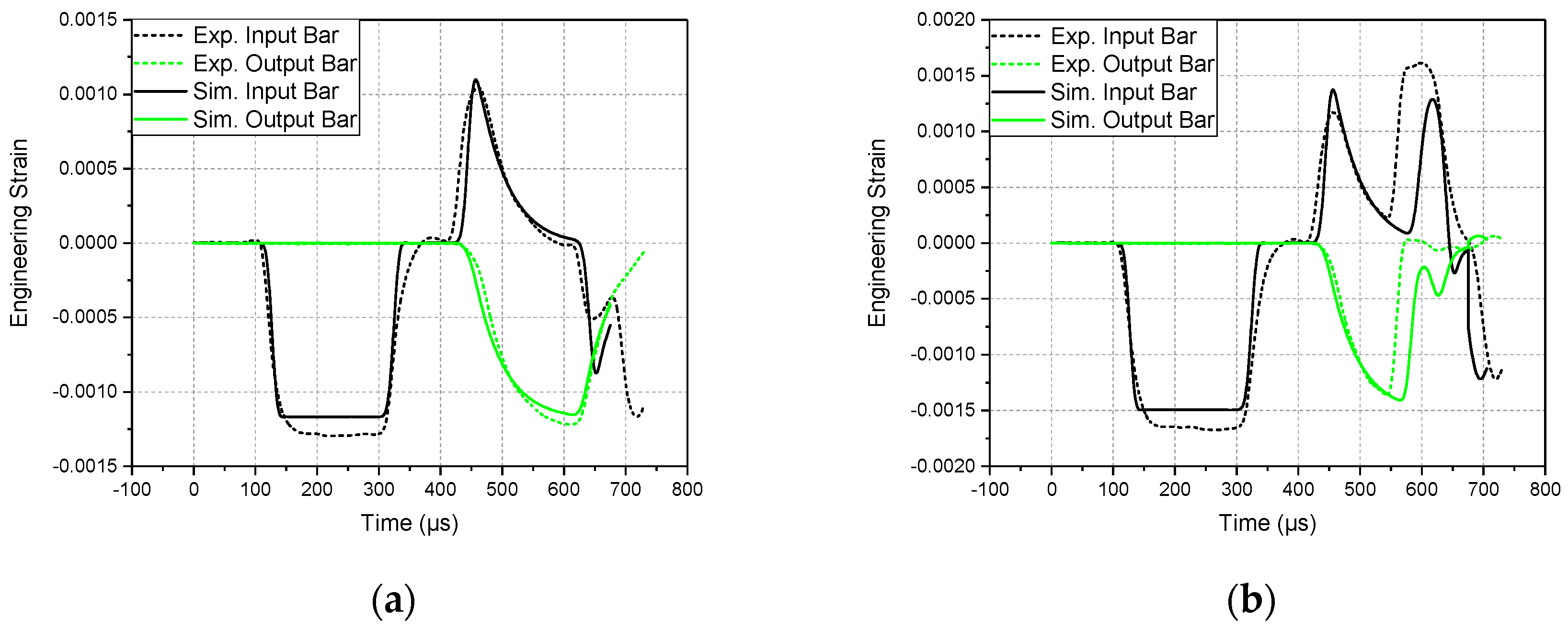
In order to compare the results with the initial wave obtained by the strain gauges in the experiments, two elements in the middle of the input and output bars were chosen to use their strain evolution as initial waves. As shown for the non-damaged and damaged situations in Figure 36a,b under 0.6 MPa and 1.0 MPa loading, respectively, the value, wave length, and trend of simulation strain were similar to the features of experiment strain.

4.1.2. Damage Kinetics

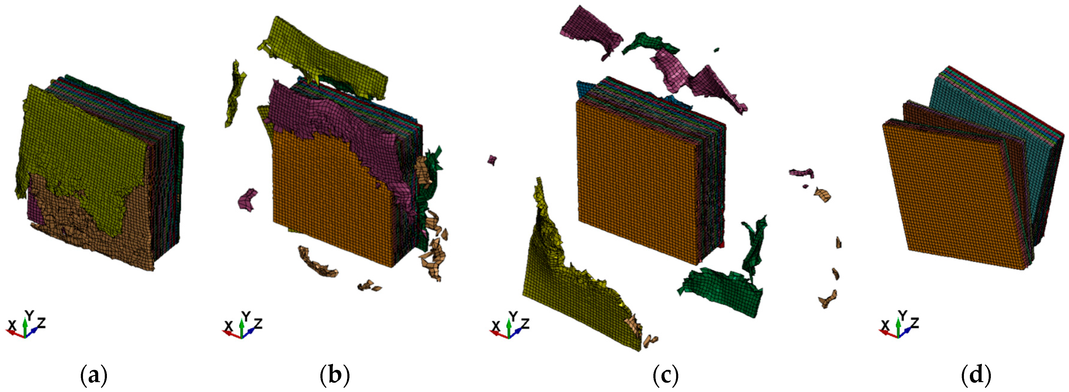
Figure 37 shows the failing process of the 8 × 8 × 8 specimen simulation under 1.0 MPa loading. Before 75 μs, the input bar moved rapidly toward the output bar. Then, they moved forward together at relatively the same velocity until 135 μs. After this moment, some sub-laminates were squeezed out and torn, becoming many fragments, as shown at 200 μs in Figure 37a–c. During this period, the output bar became still, and the input bar again moved rapidly toward the output bar. Moreover, with the input bar moving, more and more sub-laminates were squeezed out and torn, becoming fragments, as shown in Figure 37b,c. Finally, the fragments separated from the specimen, while the main body of the specimen was divided into several big blocks, as shown in Figure 37d. By comparing Figure 37 with Figure 38, it can be seen that the two features of the simulation result were similar to those of the experimental result; the layers were squeezed out and torn to fragments, while the main body of the specimen was divided into several relatively big blocks.

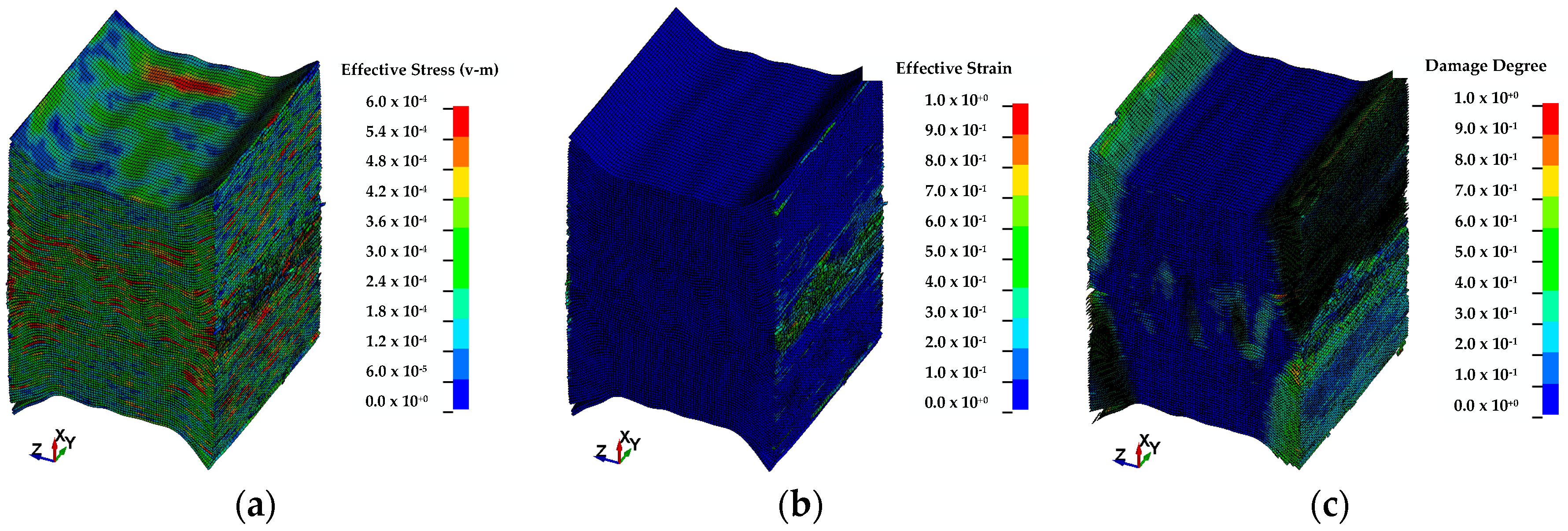
The contours of the simulation specimen at a certain moment are shown in Figure 39. As shown for the simulation specimen in Figure 39a, the effective stress distribution across the sub-laminates at the two end faces was relatively higher than the effective stress distribution at the center. As the sub-laminates at the end faces failed, some elements were deleted while some elements remained. At the edge of the remaining elements, the effective stress became lower. Correspondingly, the elements at the edge had a higher effective strain than the other elements, as shown in Figure 39b. As shown in Figure 39c, a greater misalignment between two adjacent sub-laminates resulted in a greater effective strain of the cohesive elements in the corresponding region. At this moment, the misalignment of the two adjacent sub-laminates at the end faces was greater than the misalignment at the center. Thus, the effective strain of cohesive elements near the end faces was higher. With regard to the end face at the front, the misalignment was higher at the lower left corner; thus, the effective strain of cohesive elements in this region was higher. The cohesive element was deleted when the damage degree reached 1.0.

As shown for the contours of the cylindrical specimen in Figure 40, the effective stress, effective strain, and damage degree were higher at the center than at the two end faces in contact with the bars. Therefore, the cylindrical specimen tended to fail at the center. By comparing Figure 29 and Figure 30, it can be seen that the effective strain of the cylindrical specimen was higher at the center, while the effective strain of the cubic specimen was higher at the two end faces in contact with the bars. This difference between cylindrical and cubic specimens is similar to the findings in Reference [37].

4.1.3. Effect of Strain Rate and Size

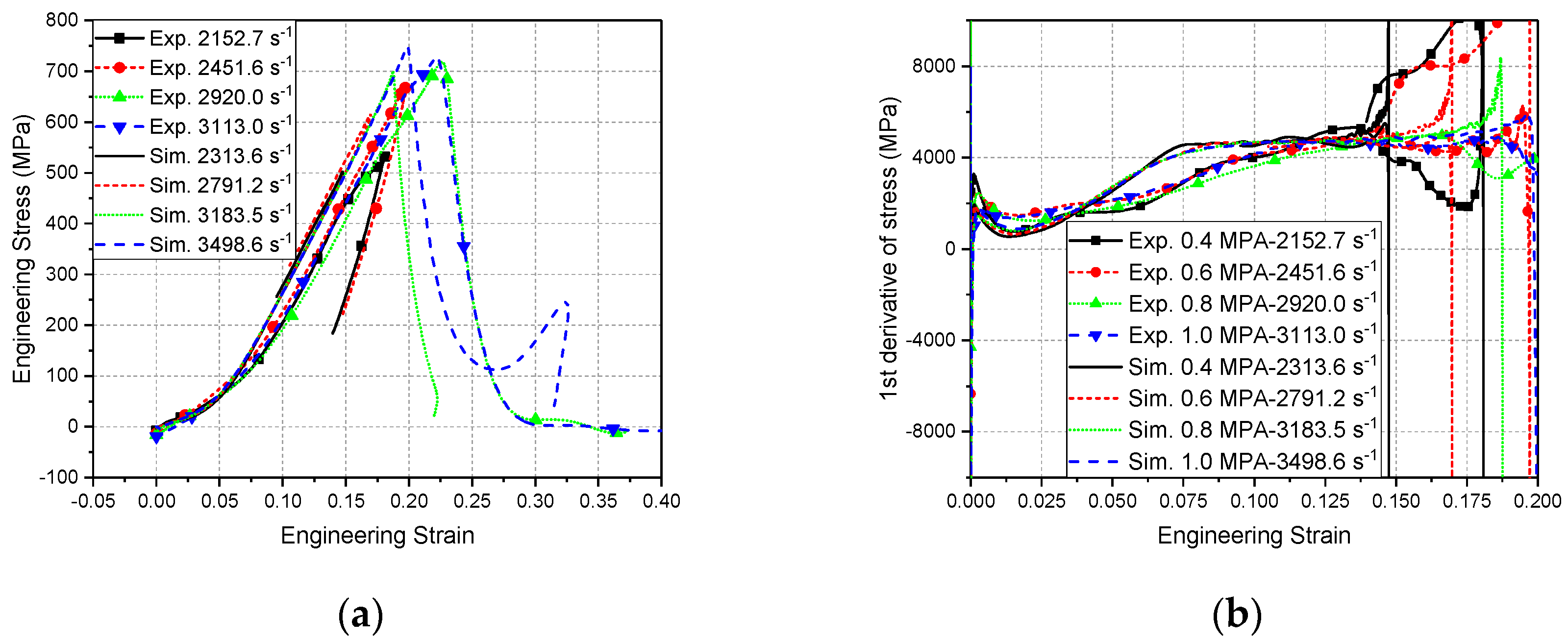
Figure 41 shows the stress–strain curves of the simulation under growing strain rates compared with the experimental result. The simulation maximum stress became higher as the strain rate became higher; this trend was the same as the experimental result. The specific simulation maximum stress values were similar to the experiment maximum stress, and the values are listed in

Table 8. The experimental (Exp)/simulation (Sim)/relative errors (RE) of strain rate and maximum stress.

Size of Specimen	Pressure	Impact Velocity	Strain Rate	Maximum Stress
mm	MPa	m/s	s−1	MPa
D-ls/L-W-ls			Exp/Sim/RE	Exp/Sim/RE
8 × 8 × 4	0.4	9.8	2160.4%/2313.6%/7.1%	535.8%/501.4%/6.4%
8 × 8 × 4	0.6	11.9667	2591.2%/2791.2%/7.7%	664.4%/615.9%/7.3%
8 × 8 × 4	0.8	13.8	3027.4%/3183.5%/5.2%	713.8%/700.0%/2.0%
8 × 8 × 4	1.0	15.3	3223.8%/3498.6%/8.5%	733.2%/747.7%/2.0%
Φ8 × 4	0.6	11.9667	2605.4%/2826.8%/8.5%	695.6%/720.6%/3.6%
Φ9 × 4	0.6	11.9667	2588.2%/2796.7%/9.3%	652.9%/621.8%/4.8%
Φ10 × 4	0.6	11.9667	2346.5%/2750.4%/17.2%	545.6%/513.7%/5.8%
Φ10 × 3	0.6	11.9667	3027.5%/3463.2%/14.4%	549.9%/510.5%/7.2%
Φ10 × 5	0.6	11.9667	2006.5%/2260.2%/12.6%	538.8%/501.0%/7.0%

. In addition, the simulation slopes of the non-linear and linear periods were similar to the experimental results. In the damaged situation shown in Figure 41a, the slope after failure was also similar to the experimental result. In the non-damaged situation shown in Figure 41a, the stress–strain curves returned after the maximum stress point along the loading path, unlike the experimental result. This was possibly because the FE model did not apply a cumulative failure model.

As the simulation results show in Figure 42a and Figure 43a, under the same impact velocity, the thickness had little influence on the maximum stress and the slope of the stress–strain curve. However, the experimental results showed that, if the specimen was thicker, the slope of the non-linear period would be higher (see Figure 14a and Figure 15a). According to Figure 35, if the specimen was more compact, the slope of the non-linear period would be higher. Therefore, this difference between the simulation and experimental results was possibly because the thicker specimen was more compact. Along the thickness of the composite plate, the middle part was more compact. The specimens could not be taken exactly from the middle part of the composite plate. As mentioned in Section 2.1, when making the specimens, one 5-mm specimen was taken from one small piece, whereas two 3-mm specimens two or 4-mm specimens were taken from one cut cube. Therefore, if the specimen was thicker, it was more likely to have a more compact part, while a thinner specimen was more likely to have a less compact part.

As the simulation results show in Figure 42b and Figure 43b, under the same impact velocity, the diameter had little influence on the slope of the stress–strain curve. If the diameter was smaller, the maximum stress would be higher. These two features were similar to the experimental result. As the simulation results show in Figure 42c and Figure 43c, under the same impact velocity, the shape of the cross-section had little influence on the maximum stress and the slope of the stress–strain curve, which is similar to the experimental result. Table 8 shows the specific values of maximum stress of different specimens. The maximum relative error was 7.3%, which indicates that the simulation results had good agreement with the experimental results.

4.2. In-Plane Simulation

4.2.1. Numerical Model

The FE model of bars and specimen is shown in Figure 44. The size of the specimen was 8 × 8 × 8 mm. The loading direction was parallel to the z-axis direction. The out-of-plane direction was parallel to the x-axis direction. The specimen was discretized into 96 sub-laminates to form the multiple layers through the thickness [4,23]. Each sub-laminate contained one layer of elements, as shown in detail in Figure 44, which represents one [0°/90°] stack. A layer of cohesive element between sub-laminates was applied [52]. As mentioned above, a small thickness was defined for the cohesive element to solve the over-penetration of elements to some extent [23]. A gap thickness of 0.001 mm was applied. Thus, the sum of all gaps was 0.095 mm, which is small (<5%) compared to the total thickness of specimen. The element size of the sub-laminate was 0.0833/0.0833/0.1667 mm. The total element amount of specimen was 880,128, in which the element amount of sub-laminates was 442,368 and the element amount of cohesive element was 437,760.

The sub-laminate was studied using the *MAT_COMPOSITE_FAILURE_SOLID_MODEL. The material parameters are shown in

Table 9. Material model properties of UHMWPE composite used in the in-plane direction [4].

Parameter: Value	Parameter: Value
Density, ρ (kg/m3) [4]: 0.97	AOPT, MACF [4]: 3.0, 3.0
Young’s modulus, Ea, Eb, Ec (GPa): 30, 30, 4.7	Tensile strengths, XT, YT, ZT (GPa) [4]: 3, 3, 3
Poisson’s ratio, νba, νca, νcb [4]: 0.06, 0.06, 0.006	Compressive strengths, XC, YC, ZC (GPa) [4]: 2, 2, 2
Shear modulus, Gab, Gbc, Gca (GPa) [4]: 4.6, 5, 5	Shear strengths, Sba, Sca, Scb (MPa): 600, 70, 70

, and they were derived from Reference [4]. According to the current slope of the experimental stress–strain curves, E_a/E_b and Ec were estimated as 30 GPa and 4.7 GPa to get better agreement with the modulus [25]. The failure of layers during this loading direction was bending, and the bending strength was smaller than the punch-shear strength. The punch-shear strength of UHMWPE laminate is ~160 MPa [4]; thus, the S_ca/S_cb applied here, which was 70 MPa and smaller than 160 MPa, could be considered acceptable. The cohesive material parameters, which were mostly derived from Reference [24], are shown in

Table 10. Material model properties of cohesive element used in out-of-plane direction [14,24].

Parameter: Value	Parameter: Value
Normal strength, T, (MPa) [14]: 1.0	Shear strength, S (MPa) [24]: 1.6
Normal stiffness, EN (MPa/mm): 40.0	Shear stiffness, ET (MPa/mm) [24]: 68.9
Energy release rate for mode I, GIC, (MPa·mm): 0.05	Energy release rate for mode II, GIIC, (MPa·mm) [24]: 0.1016

, in which T is cited from Reference [14]. G_IC and G_IIC were equal to T*E_N/2 and S*E_T/2, respectively, as shown in Figure 33.

In order to compare the results with the initial wave obtained by the strain gauges in the experiments, two elements on the middle of the input and output bars were chosen to use their strain as initial waves. As shown in Figure 45, under 0.2 MPa loading, the value, wave length, and trend of strain of the simulation results were similar to the features of experimental strain.

4.2.2. Damage Kinetics

The simulation failure process under 0.2 MPa loading is shown in Figure 46. The input bar was at the right side of the specimen. The corner of the specimen in contact with the input bar was squeezed vertically. This moment occurred at 25 μs, which was similar to the experimental 23.69 μs. After 55 μs, gaps between sub-laminates began to generate. By comparing Figure 46c at 201.38 μs with Figure 24d at 200 μs, it can be seen that both simulation and experimental results showed that some sub-laminates were separate while some were still stuck to each other. Therefore, the simulation result had good agreement with the experimental result on failure morphology. It was discussed in Reference [17] that the slight general difference in fracture form at the four corners may be related to the experimental conditions; the geometry of the samples is not perfectly cubic and, thus, the parallelism of the faces in contact with the bars is not as perfect as in the numerical model.

The contours of the simulation specimen under 0.2 MPa loading at a certain moment are shown in Figure 47. As shown in the simulation specimen in Figure 47a, the effective stress distribution at the center was relatively higher than the effective stress distribution near the vertical sub-layers. As shown in Figure 47b, the effective strain of the center at the end faces near the input and output bar had a higher value than the vertical corners and other regions of the specimen, which indicates that the elements in this region were squeezed the most. As shown in Figure 47c, a greater misalignment between two adjacent sub-layers resulted in a greater effective strain of cohesive elements in the corresponding region. At this moment, the misalignment of two adjacent sub-layers at the four vertical corners was greater than the misalignment at the center, and even greater than that in other regions. Thus, the effective strain of cohesive elements at the four corners was highest, followed by the center region. The cohesive element was deleted when the damage degree reached 1.0.

4.2.3. Effect of Strain Rate and Size

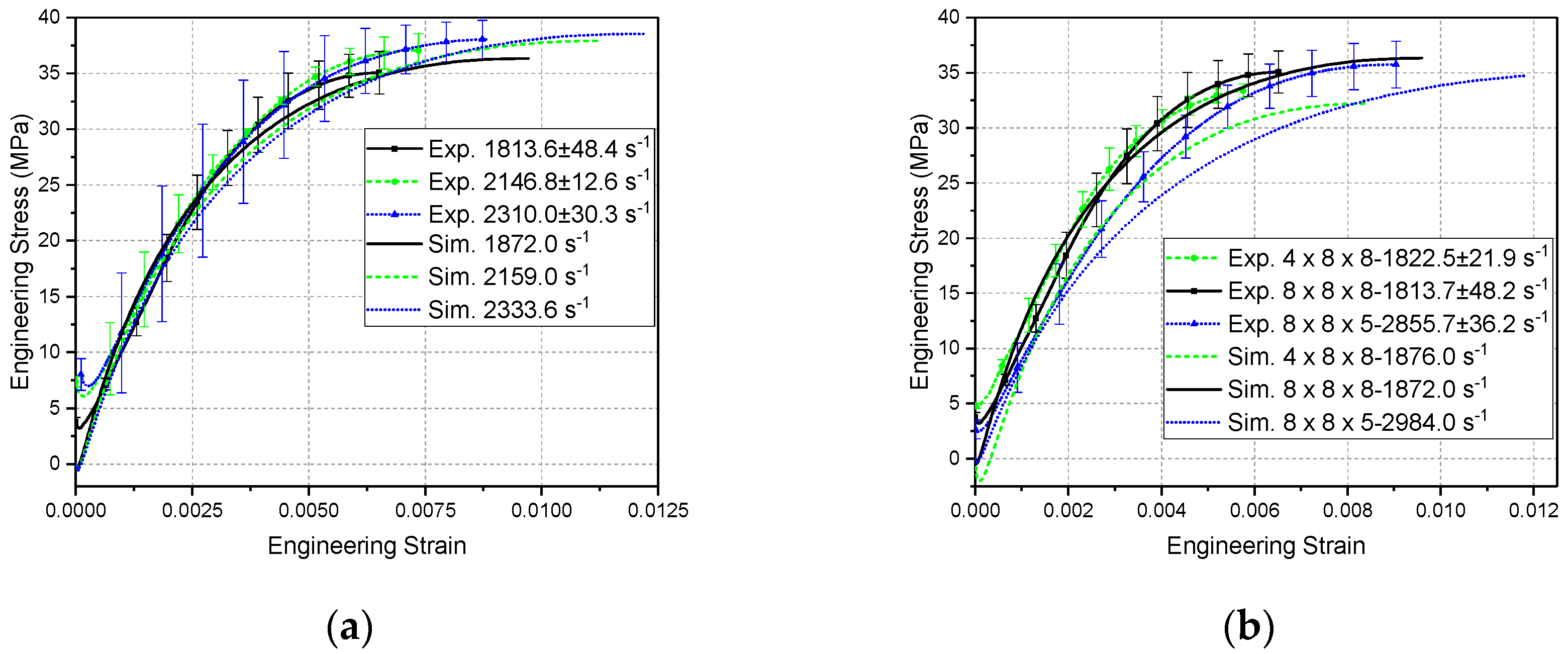
As the simulation results show in Figure 48a, with the strain rate increasing, the maximum stress increased as well. This trend was the same as the experimental trend. As shown in Figure 49a, in both simulation and experimental results, before a certain point, the slope of the stress–strain curve decreased with increasing strain rate. After this point, the slope of the stress–strain curve increased with increasing strain rate. However, the range is not great. As shown in Figure 48b and Figure 49b, both simulation and experiment results showed that, when the thickness and area became smaller, the slope values of stress–strain became lower. Moreover, the influence of thickness was greater than the influence of cross-section area. The specific maximum stress values are provided in

Table 11. The experiment/simulation/relative errors of strain rate and fracture stress.

Size of Specimen	Pressure	Impact Velocity	Strain Rate	Fracture Stress
mm	MPa	m/s	s−1	MPa
L-W-ls			Exp/Sim/RE	Exp/Sim/RE
8 × 8 × 8	0.2	15.03	1813.6%/1872.0%/3.2%	35.1%/36.3%/3.4%
8 × 8 × 8	0.3	17.35	2146.8%/2159.0%/0.6%	37.0%/37.9%/2.4%
8 × 8 × 8	0.4	18.73	2310.0%/2333.6%/1.0%	38.0%/38.6%/1.6%
4 × 8 × 8	0.2	15.03	1822.5%/1876.0%/2.9%	33.4%/32.2%/3.6%
8 × 8 × 5	0.2	15.03	2855.7%/2984.0%/4.5%	35.7%/34.7%/2.8%

. The biggest and smallest relative errors between simulation and experiment were 3.4% and 0.8%, respectively. Therefore, the simulation results had good agreement with the experimental results.

5. Conclusions

In this study, quasi-static and dynamic compressive experiments of UHMWPE laminate in the out-of-plane and in-plane directions were performed. The stress–strain relationship, the influence of different thickness, area, and shape, and the maximum stress and fracture stress were studied. The material showed a dependency on strain rate and loading direction. FE models with cohesive elements were developed. The biggest relative errors between numerical and experimental maximum stress for the out-of-plane and in-plane directions were 7.3% and 3.4%, respectively. The numerical failure form showed good agreement with the experimental form in both directions. The detailed features for different directions are concluded below.

• For both directions, the stress–strain curves had a self-installation zone and under-loading zone. In the out-of-plane dynamic tests, the loading zone of the stress–strain curve could be divided into a non-linear period and linear period. In the in-plane dynamic tests, the loading zone of the stress–strain curve could be divided into a linear period and non-linear period.
• In the out-of-plane dynamic tests, the maximum stress increased with the increasing strain rate until fracture occurred under a certain strain rate. In contrast, in the in-plane dynamic tests, the fracture happened at every tested strain rate. For both directions, the fracture stress increased with the increasing strain rate. The fracture stress of the out-of-plane dynamic tests was relatively higher than the fracture stress of the in-plane dynamic tests. In both the out-of-plane and the in-plane directions, the slope and fracture stress of the dynamic stress–strain curves were higher than the slope and fracture stress of the quasi-static stress–strain curves.
• In the out-of-plane dynamic tests and simulation, the thickness did not have a clear influence on the modulus. In the in-plane dynamic tests and simulation, the thinner specimen had a smaller modulus.
• In the out-of-plane dynamic simulation, a larger gap between sub-laminates caused the slope of the non-linear period of stress–strain curves to be shallower and longer; however, a larger gap did not clearly influence the slope of the linear period and the maximum stress. This indicates that the non-linear period was mainly caused by the compactness of the specimen.
• In the out-of-plane direction, both simulation and experiment results showed that many small fragments were squeezed out of the specimen in the damaged situation. In the in-plane direction both simulation and experiment showed that the specimens were squeezed to become big pieces.

References

1. Anderson, C.E. A review of computational ceramic armor modeling. Proceedings of the 30. In Advances in Ceramic Armor; Wiley: Hoboken, NJ, USA, 2007. [Google Scholar]
2. Zhu, Y.; Liu, G.R.; Wen, Y.; Xu, C.; Niu, W.; Wang, G. Back-Spalling process of an Al2O3 ceramic plate subjected to an impact of steel ball. Int. J. Impact Eng. 2018, 122, 451–471. [Google Scholar] [CrossRef]
3. Nguyen, L.H.; Ryan, S.; Cimpoeru, S.J.; Mouritz, A.P.; Orifici, A.C. The effect of target thickness on the ballistic performance of ultra high molecular weight polyethylene composite. Int. J. Impact Eng. 2015, 75, 174–183. [Google Scholar] [CrossRef]
4. Wen, Y.; Xu, C.; Wang, S.; Batra, R.C. Analysis of behind the armor ballistic trauma. J. Mech. Behav. Biomed. Mater. 2015, 45, 11–21. [Google Scholar] [CrossRef] [PubMed]
5. Bürger, D.; De Faria, A.R.; De Almeida, S.F.; De Melo, F.C.; Donadon, M.V. Ballistic impact simulation of an armour-piercing projectile on hybrid ceramic/fiber reinforced composite armours. Int. J. Impact Eng. 2012, 43, 63–77. [Google Scholar]
6. Sławski, S.; Szymiczek, M.; Kaczmarczyk, J.; Domin, J.; Duda, S. Experimental and Numerical Investigation of Striker Shape Influence on the Destruction Image in Multilayered Composite after Low Velocity Impact. Appl. Sci. 2020, 10, 288. [Google Scholar] [CrossRef] [Green Version]
7. Chen, L.; Zheng, K.; Fang, Q. Effect of strain rate on the dynamic tensile behaviour of UHMWPE fibre laminates. Polym. Test. 2017, 63, 54–64. [Google Scholar] [CrossRef]
8. O’Masta, M.R.; Compton, B.G.; Gamble, E.A.; Zok, F.W.; Deshpande, V.S.; Wadley, H.N.G. Ballistic impact response of an UHMWPE fiber reinforced laminate encasing of an aluminum-alumina hybrid panel. Int. J. Impact Eng. 2015, 86, 131–144. [Google Scholar] [CrossRef] [Green Version]
9. Zhang, B.; Nian, X.; Jin, F.; Xia, Z.; Fan, H. Failure analyses of flexible Ultra-High Molecular Weight Polyethylene (UHMWPE) fiber reinforced anti-blast wall under explosion. Compos. Struct. 2018, 184, 759–774. [Google Scholar] [CrossRef]
10. van der Werff, H.; Heisserer, U. High-performance ballistic fibers: Ultra-high molecular weight polyethylene (UHMWPE). In Advanced Fibrous Composite Materials for Ballistic Protection, 1st ed.; Chen, X., Ed.; Woodhead Publishing: Cambridge, UK, 2016; Chapter 3; pp. 71–107. [Google Scholar]
11. Vlasblom, M. The manufacture, properties, and applications of high-strength, high-modulus polyethylene fibers. In Handbook of Properties of Textile and Technical Fibres, 2nd ed.; Bunsel, A.R., Ed.; Woodhead Publishing: Cambridge, UK, 2018; Chapter 18; pp. 699–755. [Google Scholar]
12. Nguyen, L.H.; Lässig, T.R.; Ryan, S.; Riedel, W.; Mouritz, A.P.; Orifici, A.C. Numerical modelling of ultra-high molecular weight polyethylene composite under impact loading. Procedia Eng. 2015, 103, 436–443. [Google Scholar] [CrossRef]
13. Ong, C.W.; Boey, C.W.; Hixson, R.S.; Sinibaldi, J.O. Advanced layered personnel armor. Int. J. Impact Eng. 2011, 38, 369–383. [Google Scholar] [CrossRef]
14. Lässig, T.; Nguyen, L.; May, M.; Riedel, W.; Heisserer, U.; van der Werff, H.; Hiermaier, S. A non-linear orthotropic hydrocode model for ultra-high molecular weight polyethylene in impact simulations. Int. J. Impact Eng. 2015, 75, 110–122. [Google Scholar] [CrossRef]
15. Lu, Y.; Zhang, Q.; Xue, Y.; Liu, W.; Long, R. High-Velocity Impact Performance of Aluminum and B4C/UHMW-PE Composite Plate for Multi-Wall Shielding. Appl. Sci. 2020, 10, 721. [Google Scholar] [CrossRef] [Green Version]
16. Russell, B.P.; Karthikeyan, K.; Deshpande, V.S.; Fleck, N.A. The high strain rate response of ultra high molecular-weight polyethylene: From fibre to laminate. Int. J. Impact Eng. 2013, 60, 1–9. [Google Scholar] [CrossRef]
17. Arbaoui, J.; Tarfaoui, M.; Alaoui, A.E.M. Mechanical behavior and damage kinetics of woven E-glass/vinylester laminate composites under high strain rate dynamic compressive loading: Experimental and numerical investigation. Int. J. Impact Eng. 2016, 87, 44–54. [Google Scholar] [CrossRef]
18. Pankow, M.; Salvi, A.; Waas, A.M.; Yen, C.F.; Ghiorse, S. Split Hopkinson pressure bar testing of 3D woven composites. Compos. Sci. Technol. 2011, 71, 1196–1208. [Google Scholar] [CrossRef]
19. Sun, Y.; Zhang, D.T.; Chen, L.; Zhang, M. Experimental Investigation on Dynamic Compression Properties of UHMWPE/Vinyl Ester 2.5 Dimensional Angle Interlocked Woven Composites. J. Mater. Eng. 2011, 1, 38–42. [Google Scholar]
20. Zhou, K.; Xu, S.Y.; Xiong, J.; Mao, M.Z.; Yang, B.; Hu, H. The high strain rate compressive properties of UHMWPE interlaced biaxial weft knitted composites. J. Funct. Mater. 2009, 3, 490–493. [Google Scholar]
21. Shi, B.B.; Sun, Y.; Chen, L.; Li, J.L. Energy absorption of ultra-high molecular weight polyethylene fiber-reinforced laminates at high strain rates. Appl. Mech. Mater. 2010, 34, 1532–1535. [Google Scholar] [CrossRef]
22. Asija, N.; Chouhan, H.; Gebremeskel, S.A.; Singh, R.K.; Bhatnagar, N. High strain rate behavior of STF-treated UHMWPE composites. Int. J. Impact Eng. 2017, 110, 359–364. [Google Scholar] [CrossRef]
23. Nguyen, L.H.; Lässig, T.R.; Ryan, S.; Riedel, W.; Mouritz, A.P.; Orifici, A.C. A methodology for hydrocode analysis of ultra-high molecular weight polyethylene composite under ballistic impact. Compos. Part A Appl. Sci. Manuf. 2016, 84, 224–235. [Google Scholar] [CrossRef]
24. Bogetti, T.A.; Walter, M.; Staniszewski, J.; Cline, J. Interlaminar shear characterization of ultra-high molecular weight polyethylene (UHMWPE) composite laminates. Compos. Part A Appl. Sci. Manuf. 2017, 98, 105–115. [Google Scholar] [CrossRef] [Green Version]
25. Liu, G.; Thouless, M.D.; Deshpande, V.S.; Fleck, N.A. Collapse of a composite beam made from ultra high molecular-weight polyethylene fibres. J. Mech. Phys. Solids. 2014, 63, 320–335. [Google Scholar] [CrossRef]
26. Grujicic, M.; Arakere, G.; He, T.; Bell, W.C.; Cheeseman, B.A.; Yen, C.F.; Scott, B. A ballistic material model for cross-plied unidirectional ultra-high molecular-weight polyethylene fiber-reinforced armor-grade composites. Mater. Sci. Eng. A 2008, 498, 231–241. [Google Scholar] [CrossRef]
27. Chocron, S.; Nicholls, A.E.; Brill, A.; Malka, A.; Namir, T.; Havazelet, D.; van der Werff, H.; Heisserer, U.; Walker, J.D. Modeling unidirectional composites by bundling fibers into strips with experimental determination of shear and compression properties at high pressures. Compos. Sci. Technol. 2014, 101, 32–40. [Google Scholar] [CrossRef]
28. Kara, A.; Tasdemirci, A.; Guden, M. Modeling quasi-static and high strain rate deformation and failure behavior of a (±45) symmetric e-glass/polyester composite under compressive loading. Mater. Design. 2013, 49, 566–574. [Google Scholar] [CrossRef] [Green Version]
29. Gürgen, S.; Kuşhan, M.C. The ballistic performance of aramid based fabrics impregnated with multi-phase shear thickening fluids. Polym. Test. 2017, 64, 296–306. [Google Scholar] [CrossRef]
30. Laha, A.; Majumdar, A.; Biswas, I.; Verma, S.K.; Bhattacharjee, D. Role of fabric geometry in ballistic performance of flexible armour panels. Procedia Eng. 2017, 173, 747–754. [Google Scholar] [CrossRef]
31. Simić, D.M.; Stojanović, D.B.; Ristović, N.; Zrilić, M.; Burzić, Z.; Marjanović, M.; Uskoković, P.S.; Aleksić, R. Ballistic Composites Reinforced with Inorganic Nanotubes of Tungsten Disulfide. In Advanced Materials for Defense; Fangueiro, R., Rana, S., Eds.; Springer: Berlin, Germany, 2020; Chapter 4; pp. 35–43. [Google Scholar]
32. Li, Y.Q.; Li, X.G.; Gao, X.L. Modeling of advanced combat helmet under ballistic impact. J. Appl. Mech. 2015, 82. [Google Scholar] [CrossRef]
33. Hisley, D.M.; Gurganus, J.C.; Drysdale, A.W. Experimental methodology using digital image correlation to assess ballistic helmet blunt trauma. J. Appl. Mech. 2011, 78. [Google Scholar] [CrossRef]
34. Daryadel, S.S.; Mantena, P.R.; Kim, K.; Stoddard, D.; Rajendran, A.M. Dynamic response of glass under low-velocity impact and high strain-rate SHPB compression loading. J. Non-Cryst. Solids 2016, 432, 432–439. [Google Scholar] [CrossRef]
35. Chen, X.; Li, Y.; Zhi, Z.; Guo, Y.; Ouyang, N. The compressive and tensile behavior of a 0/90 C fiber woven composite at high strain rates. Carbon 2013, 61, 97–104. [Google Scholar] [CrossRef]
36. Chouhan, H.; Asija, N.; Gebremeskel, S.A.; Bhatnagar, N. Effect of specimen thickness on high strain rate properties of Kevlar/polypropylene composite. Procedia Eng. 2017, 173, 694–701. [Google Scholar] [CrossRef]
37. Zhong, W.Z.; Rusinek, A.; Jankowiak, T.; Abed, F.; Bernier, R.; Sutter, G. Influence of interfacial friction and specimen configuration in Split Hopkinson Pressure Bar system. Tribol. Int. 2015, 90, 1–14. [Google Scholar] [CrossRef]
38. Kapoor, R.; Pangeni, L.; Bandaru, A.K.; Ahmad, S.; Bhatnagar, N. High strain rate compression response of woven Kevlar reinforced polypropylene composites. Compos. Part B Eng. 2016, 89, 374–382. [Google Scholar] [CrossRef]
39. Kolsky, H. An investigation of the mechanical properties of materials at very high rates of loading. Proc. Phys. Soc. B 1949, 62, 676. [Google Scholar] [CrossRef]
40. Vecchio, K.S.; Jiang, F. Improved pulse shaping to achieve constant strain rate and stress equilibrium in split-Hopkinson pressure bar testing. Metall. Mater. Trans. A 2007, 38, 2655–2665. [Google Scholar] [CrossRef]
41. Larbi, G.; Mostapha, T.; Hocine, O.; Alaoui, A.E.M. A practical note for SHPB test with new algorithms for delimiting pulses. Compos. Struct. 2015, 126, 145–158. [Google Scholar] [CrossRef]
42. Hao, Y.; Hao, H.; Li, Z.X. Influence of end friction confinement on impact tests of concrete material at high strain rate. Int. J. Impact Eng. 2013, 60, 82–106. [Google Scholar] [CrossRef]
43. Li, Q.M.; Lu, Y.B.; Meng, H. Further investigation on the dynamic compressive strength enhancement of concrete-like materials based on split Hopkinson pressure bar tests. Part II: Numerical simulations. Int. J. Impact Eng. 2009, 36, 1335–1345. [Google Scholar] [CrossRef] [Green Version]
44. Jankowiak, T.; Rusinek, A.; Lodygowski, T. Validation of the Klepaczko–Malinowski model for friction correction and recommendations on Split Hopkinson Pressure Bar. Finite Elem. Anal. Des. 2011, 47, 1191–1208. [Google Scholar] [CrossRef]
45. Shang, B.; Wu, L.P.; Zhuang, Z. The effect of stress heterogeneous on test data of concrete using SHPB. Eng. Mech. 2011, 12, 33–38. [Google Scholar]
46. Mohr, D.; Gary, G.; Lundberg, B. Evaluation of stress–strain curve estimates in dynamic experiments. Int. J. Impact Eng. 2010, 37, 161–169. [Google Scholar] [CrossRef] [Green Version]
47. Zhu, J.; Hu, S.; Wang, L. An analysis of stress uniformity for concrete-like specimens during SHPB tests. Int. J. Impact Eng. 2009, 36, 61–72. [Google Scholar] [CrossRef]
48. Mostapha, T. Experimental investigation of dynamic compression and damage kinetics of glass/epoxy laminated composites under high strain rate compression. Adv. Compos. Mater.-Ecodes. Anal. 2011, 16, 359–380. [Google Scholar]
49. Haque, A.; Ali, M. High strain rate responses and failure analysis in polymer matrix composites–an experimental and finite element study. J. Compos. Mater. 2005, 39, 423–450. [Google Scholar] [CrossRef]
50. Song, Z.; Wang, Z.; Ma, H.; Xuan, H. Mechanical behavior and failure mode of woven carbon/epoxy laminate composites under dynamic compressive loading. Compos. Part B Eng. 2014, 60, 531–536. [Google Scholar] [CrossRef]
51. Song, B.; Chen, W.; Weerasooriya, T. Quasi-static and dynamic compressive behaviors of a S-2 glass/SC15 composite. J. Compos. Mater. 2003, 37, 1723–1743. [Google Scholar] [CrossRef]
52. Fleming, D.C. Modelling composite crushing initiation using a cohesive element formulation. Int. J. Crashworthiness 2011, 16, 475–485. [Google Scholar] [CrossRef]
Figure 1. The schematic structure of ultra-high-molecular-weight polyethylene (UHMWPE) laminate.
Applsci 10 01505 g001
Figure 2. Schematic diagram of Split Hopkinson pressure bar (SHPB) experimental apparatus.
Applsci 10 01505 g002
Figure 3. SHPB experimental apparatus.
Applsci 10 01505 g003
Figure 4. The quasi-static compressive behavior under out-of-plane loading: (a) stress–strain curve; (b) first derivative of stress vs. strain curve.
Applsci 10 01505 g004
Figure 5. The failure pattern of the bigger specimen: (a) top view of the two pieces; (b) shear failure feature.
Applsci 10 01505 g005
Figure 6. The failure pattern of the smaller specimen: (a) top view of the specimen; (b) inner feature of the specimen.
Applsci 10 01505 g006
Figure 7. Evolution of the stress and strain rate curves of non-damaging test under out-of-plane loading: (a) stress and strain rate vs. time curves; (b) stress vs. strain curve.
Applsci 10 01505 g007
Figure 8. Evolution of the stress and strain rate curves of damaging test under out-of-plane loading: (a) stress and strain rate vs. time curves; (b) stress vs. strain curve.
Applsci 10 01505 g008
Figure 9. The failing process of the specimen under out-of-plane loading: (a) 0 μs; (b) 20.8 μs; (c) 31.2 μs; (d) 56.16 μs; (e) 126.88 μs; (f) 520 μs.
Applsci 10 01505 g009
Figure 10. The evolution of stress with increasing strain rate.
Applsci 10 01505 g010
Figure 11. Dynamic behavior of Φ9 × 4 specimens.
Applsci 10 01505 g011
Figure 12. The changes in material properties of the Φ9 × 4 specimens with increasing strain rate: (a) max stress and energy absorption vs. strain rate curve; (b) max strain vs. strain rate curve.
Applsci 10 01505 g012
Figure 13. The morphological differences of Φ9 × 4 specimens under increasing strain rate (s−1): (a) 1666.6250 ± 2.5290; (b) 2232.7599 ± 146.0478; (c) 2588.1668 ± 164.9590; (d) 3045.0018 ± 78.6690; (e) 3210.3948 ± 121.6243; (f) 3284.0803 ± 45.5605.
Applsci 10 01505 g013
Figure 14. The stress–strain curves of different specimens: (a) effect of thickness; (b) effect of diameter/area; (c) effect of cross-section shape.
Applsci 10 01505 g014
Figure 15. The first derivative of stress–strain curves of different specimens: (a) effect of thickness; (b) effect of diameter/area; (c) effect of cross-section shape.
Applsci 10 01505 g015
Figure 16. (a) The fitted modulus of the Φ9 × 4 specimens; (b) the modulus of each size of specimen.
Applsci 10 01505 g016
Figure 17. The quasi-static and high-strain-rate test results of 8 × 8 × 4 specimens.
Applsci 10 01505 g017
Figure 18. The fracture stress and strain of the quasi-static and high-strain-rate test of 8 × 8 × 4 specimens.
Applsci 10 01505 g018
Figure 19. The quasi-static compressive behavior under in-plane loading: (a) stress–strain curve; (b) first derivative of stress vs. strain curve.
Applsci 10 01505 g019
Figure 20. The fracture pattern of the smaller specimen: (a) side view of one kind of kink band; (b) side view of another kind of kink band.
Applsci 10 01505 g020
Figure 21. The fracture pattern of the bigger specimen: (a) side view of one kind of kink band; (b) side view of another kind of kink band.
Applsci 10 01505 g021
Figure 22. The first derivative of stress vs. strain curves of 8 × 8 × 8 specimen.
Applsci 10 01505 g022
Figure 23. Evolution of the stress and strain rate curves under in-plane loading: (a) stress and strain rate vs. time curves; (b) stress vs. strain curve.
Applsci 10 01505 g023
Figure 24. The failing process of specimen under in-plane loading: (a) t = 0 μs; (b) t = 23.69 μs; (c) t = 52.12 μs; (d) t = 201.38 μs.
Applsci 10 01505 g024
Figure 25. The energy absorption of 8 × 8 × 8 specimens.
Applsci 10 01505 g025
Figure 26. The morphological differences of 8 × 8 × 8 specimens under increasing strain rate (s−1): (a) 1813.5829 ± 48.4181; (b) 2146.7858 ± 12.5833; (c) 2309.9629 ± 30.2695.
Applsci 10 01505 g026
Figure 27. The stress–strain curves of different specimens: (a) behavior of 4 × 8 × 8 specimens; (b) behavior of 8 × 8 × 8 specimens; (c) behavior of 8 × 8 × 5 specimens.
Applsci 10 01505 g027
Figure 28. The first derivative of stress–strain curves of different specimens: (a) derivative of 4 × 8 × 8 specimens; (b) derivative of 8 × 8 × 8 specimens; (c) derivative of 8 × 8 × 5 specimens.
Applsci 10 01505 g028
Figure 29. The fitted modulus of the 8 × 8 × 8 specimens.
Applsci 10 01505 g029
Figure 30. The fracture stress and strain of different specimens.
Applsci 10 01505 g030
Figure 31. The quasi-static and high-strain-rate test results of 8 × 8 × 8 specimens.
Applsci 10 01505 g031
Figure 32. The fracture stress, strain, and modulus of the quasi-static and high-strain-rate tests of 8 × 8 × 8 specimens: (a) fracture stress and strain; (b) modulus.
Applsci 10 01505 g032
Figure 33. Traction–separation law of a cohesive element.
Applsci 10 01505 g033
Figure 34. The simulated model of specimen under out-of-plane loading.
Applsci 10 01505 g034
Figure 35. The simulation results of different gap values between sub-laminates: (a) stress–strain curves; (b) first derivative of stress–strain curves.
Applsci 10 01505 g035
Figure 36. The experimental and simulated initial waves under out-of-plane loading: (a) non-damaged situation under 0.6 MPa loading; (b) damaged situation under 1.0 MPa loading.
Applsci 10 01505 g036
Figure 37. The simulated failure process of the specimen under out-of-plane loading: (a) 155 μs; (b) 170 μs; (c) 200 μs; (d) 410 μs.
Applsci 10 01505 g037
Figure 38. The fracture pattern of 8 × 8 × 4 specimens under 1.0 MPa loading.
Applsci 10 01505 g038
Figure 39. The contours of 8 × 8 × 8 specimen at 155 μs (unit: cm-μs-g): (a) effective stress of sub-laminates; (b) effective strain of sub-laminates; (c) damage degree of cohesive elements.
Applsci 10 01505 g039
Figure 40. The contours of Φ9 × 4 specimen at 125 μs (unit: cm-μs-g): (a) effective stress of sub-laminates; (b) effective strain of sub-laminates; (c) damage degree of cohesive elements.
Applsci 10 01505 g040
Figure 41. The experimental and simulation results under different strain rates: (a) stress–strain curves; (b) first derivative of stress–strain curves.
Applsci 10 01505 g041
Figure 42. The experimental and simulated stress–strain curves of different specimens under the same impact velocity: (a) effect of thickness; (b) effect of diameter/area; (c) effect of cross-section shape.
Applsci 10 01505 g042aApplsci 10 01505 g042b
Figure 43. The experimental and simulated first-derivative curves of different specimens under the same impact velocity: (a) effect of thickness; (b) effect of diameter/area; (c) effect of cross-section shape.
Applsci 10 01505 g043
Figure 44. The simulated model of specimen under in-plane loading.
Applsci 10 01505 g044
Figure 45. The experimental and simulated initial waves under in-plane loading.
Applsci 10 01505 g045
Figure 46. The simulated failing process of the specimen under in-plane loading: (a) 25 μs; (b) 55 μs; (c) 200 μs.
Applsci 10 01505 g046
Figure 47. The contours of the specimen at 55 μs (unit: cm-μs-g): (a) effective stress of sub-laminates; (b) effective strain of sub-laminates; (c) damage degree of cohesive elements.
Applsci 10 01505 g047
Figure 48. The experimental and simulated stress–strain curves of different specimens under same impact velocity: (a) effect of strain rate (8 × 8 × 8); (b) effect of different size.
Applsci 10 01505 g048
Figure 49. The experimental and simulated first-derivative curves of different specimens under same impact velocity: (a) effect of strain rate (8 × 8 × 8); (b) effect of different size.
Applsci 10 01505 g049