An Improvement on Estimated Drifter Tracking through Machine Learning and Evolutionary Search

Abstract

In this study, we estimated drifter tracking over seawater using machine learning and evolutionary search techniques. The parameters used for the prediction are the hourly position of the drifter, the wind velocity, and the flow velocity of each drifter position. Our prediction model was constructed through cross-validation. Trajectories were affected by wind velocity and flow velocity from the starting points of drifters. Mean absolute error (MAE) and normalized cumulative Lagrangian separation (NCLS) were used to evaluate various prediction models. Radial basis function network showed the lowest MAE of 0.0556, an improvement of 35.20% over the numerical model MOHID. Long short-term memory showed the highest NCLS of 0.8762, an improvement of 6.24% over MOHID.

1. Introduction

The worldwide increase of large ships and maritime transportation volume causes a number of accidents that are beyond the capacity of individual nations. Pollutants released from accidents may extensively contaminate the marine environment due to ocean currents, weather, and weathering. Therefore, pollutants released during an accident should be removed as soon and as much as possible. An accurate prediction of the pollutant movement can help track and address them, as a variety of studies have proven [1,2,3,4,5]. The prediction model for oil spills generally calculates the movement and spread of the oil spill using the Lagrangian particle approach [5,6,7]. This forecasting method uses physics for critical parameters such as flow velocity, wind velocity, water level, and temperature in the current state. Parameter optimization using evolutionary computation [8] showed better results than MOHID [6], a numerical water modelling system. Machine learning and ensemble methods [9,10] were also used to estimate the movement of drifters.

Predicting the movement of a drifter on the ocean is an essential step in tracking the spread of an oil spill [11]. While spilled oil may sink or evaporate, most of it floats on the surface. Conventional numerical models can predict oil spills more accurately if the trajectories of drifting particles can be predicted accurately. Therefore, we aimed to predict more accurate trajectories by using various machine learning methods including deep learning, which has attracted much recent attention, rather than by using evolutionary computation as in our previous study [8]. We integrated artificial intelligence (AI) technology to predict the future ocean state, utilizing the continuity of parameter data over time. We expanded the area covered by our previous study [8], which predicted the trajectory of drifting objects in the ocean and systematically compared a wide range of regression functions and artificial neural networks for predicting the movement of drifters. In order to avoid the look-ahead bias, we used wind and flow forecasts made by the Korea Meteorological Administration and private technical agencies instead of actual future parameters.

In sum, the contributions of this study are summarized as follows. We applied evolutionary computation and machine learning to the prediction of drifter trajectories. We extended and improved our previous study [8] that used evolutionary computation, and we also first predicted the trajectories using various machine learning techniques. This study was the first time that machine learning techniques have been applied to the prediction of drifter trajectories—before this study, only numerical models such as MOHID have been applied to drifter trajectories. Our methods could significantly improve on the results of the representative numerical model, MOHID.

2. Literature Review

ADIOS [12], developed by the United States in the early 1990s, is one of the widely used decision-making support systems for spilled oil. These support systems share the characteristics of simplicity, high performance, open-source programming, and an extensive oil database. The performance of ADIOS has continued to improve [13] and provides a basis for newly developed oil weathering models. Unfortunately, it cannot use data on the current state [14] and simulate the trajectory of the oil spill. The ADIOS model requires information on spilled oil situations, environmental conditions and prevention strategies, and calculates optimal prediction results by inputting minimum information obtained or expected in the field.

The prediction models for oil spill movements were developed for accurate and detailed analysis. Oil companies, consulting sectors, national agencies, and research centers use certain models worldwide, which enable them to input various marine weather and environmental data to consider oil weathering, and are thus suitable for planning stages and research scenarios for different types of oil and marine weather conditions. Related models are GNOME [7], OILMAP [15] OSCAR [16], OSIS, GULFSPILL [17], MOHID [6], etc. Among them, MOHID [6], which is used as a benchmark measure of performance in this study, was first developed in 1985 at the Marine and Environmental Technology Research Center (IST) of the Instituto Superior Técnico (IST), affiliated with the University of Lisbon, Portugal. MOHID is a multifunctional three-dimensional numerical analysis model that can be applied to coastal and estuary areas, which basically calculates physical actions in coastal and estuary areas such as tide and tsunami. It consists of more than 60 modules that can calculate fluid properties (water temperature, salinity, etc.), Lagrangian movement, turbulence, sediment movement, erosion and sedimentation, meteorological and wave conditions, water quality and ecology, and oil diffusion.

Recent advancements in operational maritime, weather forecasting, and computing technologies have allowed for automated prediction in desktop and web environments. Such prediction models include MOTHY [18], POSEIDON OSM [19], MEDSLICK [20], MEDSLICK II [5], OD3D [21], LEEWAY [22], OILTRANS [14], BSHmod.L [23], and SEATRACK Web [24]. Some models cannot process 3D ocean data or consider stokes drift and the vertical movement of droplets. Research is underway to provide user requirements, convenient and comprehensive user-friendly environments, and geographic information system (GIS) results to improve the model landscape.

Typical models that predict Lagrangian drifter trajectory are known to be less accurate for large structures [25]. Therefore, Aksamit et al. [25] used long short-term memory (LSTM) to accurately predict the velocity of drifters. They used the drifter data obtained from the Gulf of Mexico. Their model was much more accurate than the model using the Maxey–Riley equation [26] in terms of root mean square error (RMSE).

3. Data

Our previous study [8] used data obtained from Seosan, located on the west coast of South Korea. For this work, we added new data obtained from Jeju Island to the previous data. Hourly data from 2015 to 2016 at these locations were used for our study. We used this to predict the hourly locations of drifters in this study. Figure 1 shows the observed trajectories from the two locations in 2015, and Table 1 shows the features related to the start and end points of trajectories of the sample data. The height of the wind velocity above the ocean was 10 m, and its spatial resolution was 900 m.

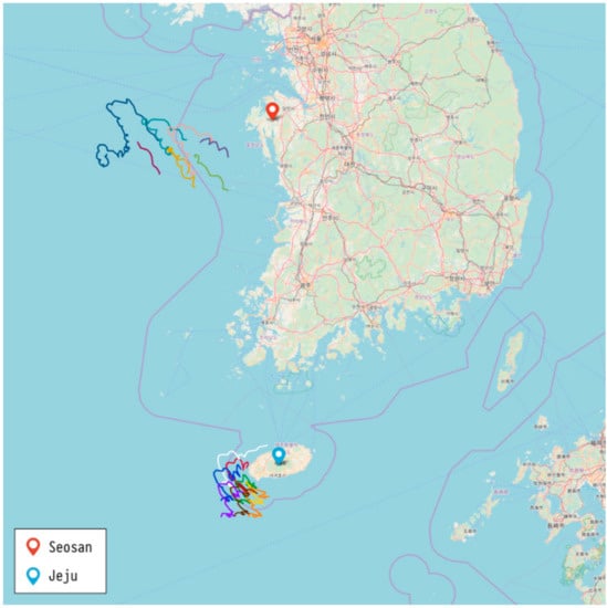
Figure 1. Observed trajectory data from Seosan and Jeju in 2015.

Table 1. Attributes of the data (examples).

Location	Case No.	#Data	Start						End
			Y	M	D	H	Lon.	Lat.	Y	M	D	H	Lon.	Lat.
Seosan	1	239	2015	11	6	8	125.0795	36.5788	2015	11	16	6	124.4480	36.4438
	2	26	2015	11	6	9	125.0858	36.2526	2015	11	7	13	124.8229	36.5638
	5	109	2015	11	6	15	125.4192	36.2578	2015	11	11	3	125.5130	36.1293
	6	112	2015	11	6	16	125.4081	36.5825	2015	11	11	7	125.1982	36.4487
	7	113	2015	11	6	17	125.7388	36.5810	2015	11	11	9	125.4705	36.2202
	8	39	2015	11	6	18	125.9147	36.4168	2015	11	8	8	125.5818	36.5624
	9	45	2015	11	6	13	125.9123	36.0874	2015	11	8	9	125.5238	36.4135
Jeju	1	82	2016	4	18	23	126.0006	33.1695	2016	4	22	8	126.1397	33.3354
	2	106	2016	4	18	23	125.8375	33.1774	2016	4	23	8	126.3886	33.5580
	3	106	2016	4	18	22	125.8338	33.0041	2016	4	23	7	126.0698	33.3213
	4	87	2016	4	19	0	126.0045	33.0026	2016	4	22	14	126.2295	33.1773
	5	60	2016	4	19	0	126.1655	33.9999	2016	4	21	11	126.1255	33.1871
	6	93	2016	4	18	20	126.1671	32.8383	2016	4	22	16	126.4106	33.0411
	7	94	2016	4	18	21	125.9990	32.8439	2016	4	22	18	12.2667	33.0728
	8	93	2016	4	18	21	125.8346	32.8395	2016	4	22	17	126.0957	33.0810

4.1. Numerical Model and Evolutionary Methods

We used MOHID [6] as a numerical model using the Navier-Stokes equations [27], and we also examined various evolutionary methods from our previous study [8]. The evolutionary methods include differential evolution (DE) [28], particle swarm optimization (PSO) [29], and the covariance matrix adaptation evolutionary strategy (CMA-ES) [30].

4.2. Machine Learning

We used supervised learning to find the mapping between input data (wind velocity and flow velocity) and output data (drifter location). The performance of the following two regression functions were examined.

Support vector regression (SVR): While conventional classifiers minimize error rates during the training process, support vector machines (SVMs) construct a set of hyperplanes so that the distance from it to the nearest training data point is maximized. They were considered as alternatives to artificial neural networks in the 1990s since nonlinear classification became possible through the kernel trick [31]. Support vector regression uses SVM for regression with continuous values as the output [32].

Gaussian process (GP): GP [33] is an ML model that predicts data as the average and variance of probability distributions. It predicts functions that can represent given data in the defined function distribution and estimates functions for experimental data based on the arbitrary training data.

4.3. Artificial Neural Networks

Artificial neural networks represent a learning algorithm inspired by the neural networks of biology. With the recent advancement of deep learning, the use of artificial neural networks has yielded excellent performance in classification and can be used for regression when a mean-square error (MSE) is the loss function. Below are the neural network methods we used in this study.

Multi-layer perceptron (MLP) is a basic neural network structure that adds hidden layers into the perception structure. We built a hierarchical model with four inputs, two outputs, and one hidden layer.

Radial basis function network (RBFN) is a type of neural network that represents the proximity to the correct answer using Gaussian probability and Euclidian distance [34]. One hidden layer based on Gaussian probability distribution is used, and the training process is extremely fast.

Deep neural network (DNN) increases training parameters by adding hidden layers in MLP. Figure 2 shows the settings of the input and output values in the basic DNN structure. It is often essential to use a rectified linear unit (ReLU) [35] and Dropout [36] to prevent the vanishing gradient problem [37].

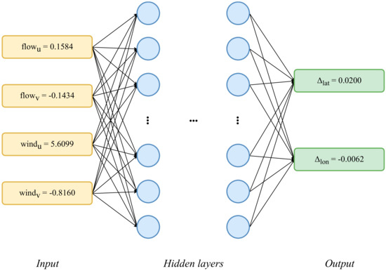
Figure 2. Data input/output in our deep neural network (DNN) model.

Recurrent neural network (RNN): the connection between units is characterized by a circular structure [38] and can be used when continuous data is given. RNNs can be used to predict trajectories since the movement of a drifter is sequential data. The input data for MLP or DNN has a fixed size of 4, as depicted in Figure 2. However, RNNs should incorporate all the drifter moves in sequence; thus, the data length can be different. The maximum length that the model can receive as an input sequence is set, and the remaining data space is padded with zero. For example, if the maximum length is set to 200 and given data set has 120 h of movement information, the remaining data is filled with 80 zeros. Figure 3 shows the input and output data structure of the RNN model.

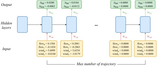
Figure 3. Data input/output in our recurrent neural network (RNN) model.

Long short-term memory (LSTM): the RNN model creates the next unit based on product operation and suffer from the vanishing gradient problem when dealing with long data sequences. LSTM [39], which has the function of forgetting past information and of remembering current information by adding a cell-state to the hidden state of RNN, has emerged as one of the most widely used RNN methods and can effectively solve not only the vanishing gradient problem but the long-term dependency. This model is expected to remember the movement of a drifter according to the specific short sequence of wind and flow.

5. Experiments

5.1. Setting and Environments

We implemented the evolutionary computation methods using DEAP software (https://deap.readthedocs.io/en/master/) except for PSO. For PSO, we used PySwarms (https://pyswarms.readthedocs.io/en/latest/), which performed better than DEAP. We used WEKA 3 [40] for MLP, GP, SVR, and RBFN, and PyTorch [41] for DNN, RNN, and LSTM. Table 2 summarizes software libraries we used.

Table 2. Methods and library resources.

Method	Library
Covariance Matrix Adaptation Evolutionary Strategy (CMA-ES)	DEAP
Differential Evolution (DE)	DEAP
Particle Swarm Optimization (PSO)	PySwarms
Multi-Layer Perceptron MLP	WEKA 3
Gaussian Process (GP)	WEKA 3
Support Vector Regression (SVR)	WEKA 3
Radial Basis Function Network (RBFN)	WEKA 3
Deep Neural Network (DNN)	PyTorch
Recurrent Neural Network (RNN)	PyTorch
Long Short-Term Memory (LSTM)	PyTorch

The previous methods of evolutionary computation evaluated test data by creating a single model per method. When a single method yields several models, the performance may vary depending on the random seed. We confirmed that there are considerable performance differences between models using the same method for deep learning methods. We used the bagging [42] method to analyze each method by creating 10 models for each method and then measuring the average value, variance, and standard deviation of the resulting measured values. There might be sharp loss value changes in the process of solving local minimum problems for deep learning methods. We calculated mean absolute error (MAE) according to epoch and ended training when the MAE value was low in our experiments.

5.2. Evaluation Measures

We used mean absolute error (MAE) and normalized cumulative Lagrangian separation (NCLS). In prior work [8], we also used the Euclidean distance as an evaluation measure. Since it is calculated by a mechanism similar to MAE, the average of the error distance was calculated only using MAE. NCLS, also called the skill score, was calculated by subtracting the error from 1. Lower values, therefore, represent better results for MAE, whereas higher values close to 1 represent better results for NCLS. The calculation for MAE can be expressed as the following Equation.

$$\frac{1}{m}{\displaystyle \sum }_{i=1}^m\left(| pred\_La{t}_i - observed\_La{t}_i|+|pred\_Lo{n}_i - observed\_Lo{n}_i|\right)$$

(1)

where pred_Lon and pred_Lat represent the longitude and latitude of the predicted data. Observed_Lon and observed_Lat denote the longitude and the latitude of the observed data. Therefore, the difference between these values can be considered as an error. The denominator m is the number of test datasets. Therefore, the MAE is the average of the errors.

NCLS is a measurement method that is quite frequently used in trajectory modeling and it is proposed to solve weaknesses in the Lagrangian separation distance in relation to the continental shelf and its adjacent deep ocean. The error of each location is calculated in MAE, whereas NCLS calculates errors by cumulative calculation. Figure 4 shows the calculation process of NCLS. In this process, if s becomes too large, the skill score may continue to remain zero. If the tolerance threshold n is set high, this can be solved to some extent. In this study, we set n to 1 since errors sufficient to make s relatively large did not frequently occur.

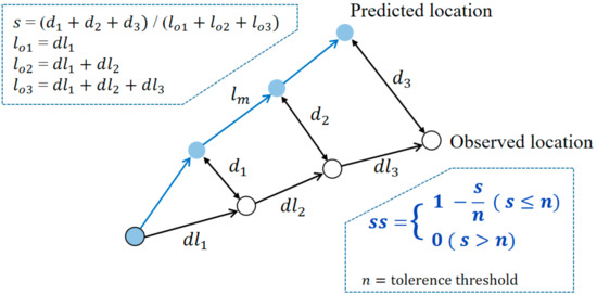
Figure 4. Formula to calculate skill score (ss) of NCLS.

5.3. Results

Previous measurements are available for evolutionary computational methods. In Section 5.3.1, we verified the performance of the Python-based system by comparing the results with only the Seosan data. The degree of training is also an essential factor. Prior to experimenting with all the data, in Section 5.3.2, we measured epoch numbers deemed good enough to end training by measuring MAE for each epoch in each deep learning method. Lastly, in Section 5.3.3, we trained them using all the data and described the experimental results that predicted the trajectories of the newly added Jeju data.

5.3.1. Evolutionary Search on Seosan Data

Table 3 compares the results of the previous study (C language) [8] and this study (Python). CMA-ES showed particularly good performance compared to the previous study. Overall, we could improve the performance of evolutionary search by using new software libraries.

Table 3. Parameters of evolutionary computation methods.

Method	Evaluation	Case
		1	5	6	7
DE (Previous)	MAE	0.0920	0.0828	0.0392	0.0653
	NCLS	0.9026	0.7965	0.9220	0.8826
DE	MAE	0.0587	0.0973	0.0380	0.0568
	NCLS	0.9451	0.7686	0.9225	0.8974
PSO (Previous)	MAE	0.0907	0.0820	0.0385	0.0622
	NCLS	0.9044	0.7984	0.9232	0.8878
PSO	MAE	0.0603	0.0973	0.0380	0.0567
	NCLS	0.9441	0.7686	0.9226	0.8976
CMA-ES (Previous)	MAE	0.1303	0.1393	0.0761	0.1304
	NCLS	0.8631	0.6513	0.8437	0.7297
CMA-ES	MAE	0.0582	0.0973	0.0380	0.0567
	NCLS	0.9457	0.7686	0.9226	0.8976
MOHID model [10]	MAE	0.1352	0.1238	0.0656	0.0434
	NCLS	0.8633	0.7134	0.8480	0.9229

The lower the mean absolute error (MAE) values, the better. The higher the NCLS values, the better.

Table 4 shows the CPU time to build the prediction models for Seosan data. Since inference time is usually much shorter than training time, actual performance can be more important than training speed.

Table 4. Computing time of evolutionary computation methods.

Data		Case 1	Case 5	Case 6	Case 7
Computing time (CPU second)	DE	2120.8	2705.8	2663.2	3066.2
	PSO	302.5	345.7	344.9	371.5
	CMA-ES	117.5	152.8	152.9	173.9

5.3.2. Deep Learning

The neural network methods use the loss value to calculate how well a model is trained. The loss value decreases as the model accurately predicts the training data. It is better to use cross-entropy and softmax in the final layer of neural network-based classifiers [43]. However, we used MSE as the loss function since we predicted continuous values, not discrete ones.

The loss function measures the difference between the correct answer of the training data and the value predicted by the model, which may not relate to MSE and NCLS. In order to identify whether or not loss and MAE are related to each other, we examined several neural network models. Neural networks learn the values of the weights to reduce loss, and a reduction of MSE can prove worthwhile. We investigated the loss according to epoch, MAE, and MAE of the test data in the three deep learning methods, CNN, RNN, and LSTM. From Jeju data, Case 1 was used as the test data, and the rest were used as training data. Figure 5 shows the results of DNN.

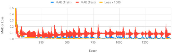
Figure 5. MAE and Loss of DNN.

DNN calculates the error between individual data independently. As the training progresses, the loss value generally decreases. However, the MAE of the training data and test data decreases sharply only at the beginning, and the performance does not significantly improve thereafter. We looked for an additional way to solve this problem, since the MAE deviation between each epoch is large even when the training is complete. We attempted to solve the problem by bagging among the ensemble techniques. The final epoch of DNN is set to 1500. The MAE of the test data was low in the 100–200 epoch section when training was incomplete, and the MAE deviation between epochs was large even post-training in the case of DNN. After 1500 epochs, the loss value did not decrease further, so we set the final epoch of DNN to 1500.

Figure 6 shows the MAE and loss values of RNN. The data are continuous time-series data of the movement of a drifter over time. Although the loss value is reduced above 100 epochs, the MAE of the training and test data did not decrease. We set the final epoch of RNN to 1000. LSTM was similar to RNN, but there were ups and downs on the MAE graph as learning progressed. The final epoch of the LSTM was set to 500. Figure 7 shows the MAE and loss values of LSTM.

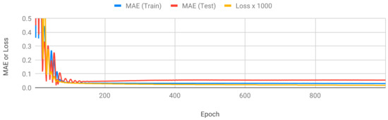
Figure 6. MAE and loss values of RNN.

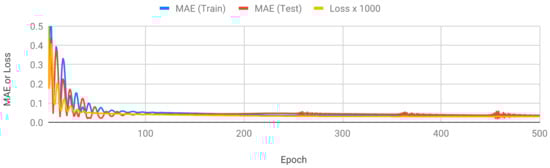
Figure 7. MAE and loss values of LSTM.

5.3.3. Results for Each Case

We describe the performance measurement results of methods beyond the evolutionary computation mentioned in Section 3. Table 5 shows the main parameter values for each method. Our prior work [8] measured the error per iteration. The deep leaning method using PyTorch (e.g., DNN, RNN, and LSTM) is conceptually similar; MAE and loss were measured per epoch. The result based on the WEKA library could not measure the error according to the iteration since it could not set the iteration number internally.

Table 5. Parameter values for machine learning (ML) methods.

Method	Parameter	Value
GP (WEKA 3)	Filter type	Standardized training data
	Level of Gaussian noise	1.0
	Decimal places	2
MLP (WEKA 3)	Activation function	Approximate sigmoid
	Loss function	Square error
	Decimal places	2
	Number of hidden units	1
	Ridge	0.01
	Tolerance	1.0 × 10−6
RBFN (WEKA 3)	Decimal places	2
	Number of basis functions	2
	Ridge	2
	Scale optimization	Use scale per unit
	Tolerance	1.0 × 10−6
SVR (WEKA 3)	Complexity constant	3.0
	Filter type	Standardized training data
	Kernel	Polynomial kernel
	Decimal places	2
DNN (PyTorch)	Loss function	Mean square error
	Activation function	ReLU
	Number of epochs	1500
	Number of hidden layers	8
	Number of units per a layer	256
RNN (PyTorch)	Loss function	Mean square error
	Number of hidden units	256
	Number of epochs	1000
LSTM (PyTorch)	Loss function	Mean square error
	Number of hidden units	256
	Number of epochs	500

Table 6 shows the evaluation of measured values by building models from ML and evolutionary computation methods. Only the Seosan data was used for training. GP, MLP, RBFN, and SVR based on WEKA showed outstanding performance. However, the deep learning methods did not perform very well as the variation in data volume by case was large for the Seosan data. The difference between the numbers of Cases 1 and 2 was nine times, as shown in Table 1. The data length also has a significant impact on training because the previous event influences the next event in RNN. Table 7 shows the CPU time spent building models for each method. Evolutionary computation methods took more time than GP, MLP, and RFBN using WEKA software.

Table 6. Results for Seosan data.

Method	Evaluation	Case
		1	5	6	7
DE	MAE	0.0743	0.0286	0.0906	0.0417
	NCLS	0.9308	0.7377	0.7769	0.9172
PSO	MAE	0.1238	0.0318	0.1050	0.0758
	NCLS	0.8724	0.7183	0.7557	0.8375
CMA-ES	MAE	0.0743	0.0286	0.0909	0.0418
	NCLS	0.9308	0.7378	0.7763	0.9170
GP	MAE	0.0945	0.0290	0.0974	0.0360
	NCLS	0.9113	0.7431	0.7583	0.9282
MLP	MAE	0.0957	0.0285	0.1012	0.0320
	NCLS	0.9030	0.7541	0.7474	0.9353
RBFN	MAE	0.1064	0.0278	0.0986	0.0297
	NCLS	0.8992	0.7626	0.7508	0.9399
SVR	MAE	0.0700	0.0301	0.0939	0.0394
	NCLS	0.9355	0.7402	0.7711	0.9204
DNN	MAE	0.1557	0.0192	0.1305	0.0571
	NCLS	0.8493	0.8383	0.6879	0.8848
RNN	MAE	0.1369	0.0270	0.1335	0.0494
	NCLS	0.8555	0.7699	0.6809	0.8910
LSTM	MAE	0.0744	0.0295	0.1153	0.0301
	NCLS	0.9201	0.7413	0.7075	0.9408
MOHID	MAE	0.1352	0.1238	0.0656	0.0434
	NCLS	0.8633	0.7134	0.8480	0.9229

The lower the MAE values, the better. The higher the NCLS values, the better.

Table 7. Computing time for Seosan data.

Data		Case 1	Case 5	Case 6	Case 7
Computing time (CPU second)	DE	2120.78	2705.83	2663.18	3066.16
	PSO	302.53	345.69	344.87	371.54
	CMA-ES	117.53	152.80	152.93	173.92
	GP	9.12	13.62	14.78	13.82
	MLP	4.45	4.33	4.50	4.60
	RBFN	3.69	3.72	3.77	3.86
	SVR	9.57	15.00	13.89	14.37
	DNN	153.36	182.26	174.52	178.29
	RNN	45.93	47.58	44.56	48.27
	LSTM	34.47	45.59	44.32	46.46

Table 8 shows the experiment results with the Jeju data. Unlike the result of the Seosan data, the deep learning methods showed excellent performance. LSTM performed better than the basic RNN models, and sometimes DNN performed better. In Cases 1, 2, and 3, MLP and RBFN using WEKA software indicated good performance, whereas the evolutionary computation methods are neither good nor bad performance. The results of the RNN methods could be improved since the variation of the number of data by case is small for the Jeju data. Table 9 shows the CPU time for calculation. The computation time for the Jeju data was not much different from that of the Seosan data.

Table 8. Results for Jeju data.

Method	Evaluation	Case
		1	2	3	4	5	6	7	8
DE	MAE	0.0497	0.0703	0.0500	0.0576	0.0337	0.0460	0.0495	0.0638
	NCLS	0.8685	0.8698	0.8930	0.8675	0.8770	0.8763	0.8805	0.8594
PSO	MAE	0.0491	0.0699	0.0501	0.0578	0.0331	0.0461	0.0480	0.0646
	NCLS	0.8702	0.8700	0.8927	0.8671	0.8785	0.8760	0.8855	0.8576
CMA-ES	MAE	0.0491	0.0702	0.0502	0.0575	0.0338	0.0461	0.0494	0.0640
	NCLS	0.8700	0.8699	0.8927	0.8677	0.8767	0.8761	0.8807	0.8589
GP	MAE	0.0447	0.0468	0.0450	0.0701	0.0273	0.0583	0.0676	0.0836
	NCLS	0.8912	0.9096	0.9115	0.8420	0.8981	0.8466	0.8439	0.8202
MLP	MAE	0.0345	0.0571	0.0398	0.0586	0.0271	0.0599	0.0669	0.0816
	NCLS	0.9145	0.8883	0.9191	0.8663	0.8988	0.8488	0.8482	0.8224
RBFN	MAE	0.0468	0.0418	0.0382	0.0632	0.0268	0.0493	0.0564	0.0723
	NCLS	0.8871	0.9192	0.9249	0.8583	0.8996	0.8727	0.8737	0.8438
SVR	MAE	0.0378	0.0542	0.0442	0.0581	0.0335	0.0507	0.0495	0.0721
	NCLS	0.9073	0.8970	0.9099	0.8683	0.8769	0.8607	0.8801	0.8432
DNN	MAE	0.0453	0.0931	0.0384	0.0487	0.0364	0.0459	0.0352	0.0436
	NCLS	0.8850	0.8193	0.9218	0.8823	0.8629	0.8849	0.9164	0.9007
RNN	MAE	0.0483	0.0635	0.0554	0.0595	0.0506	0.0661	0.0414	0.0647
	NCLS	0.8787	0.8710	0.8840	0.8510	0.8226	0.8346	0.8935	0.8504
LSTM	MAE	0.0478	0.0608	0.0526	0.0445	0.0338	0.0362	0.0411	0.0451
	NCLS	0.8841	0.8812	0.8907	0.8953	0.8793	0.9071	0.9076	0.9012
MOHID	MAE	0.0622	0.0630	0.0883	0.1043	0.0236	0.0724	0.0864	0.1116
	NCLS	0.8361	0.8792	0.8271	0.7559	0.9140	0.8324	0.8007	0.7585

Table 9. Computing time for Jeju data.

Data		Case 1	Case 2	Case 3	Case 4	Case 5	Case 6	Case 7	Case 8
Computing time (CPU second)	DE	3004.0	2879.6	2900.4	2956.5	3098.1	2966.9	2978.2	2958.7
	PSO	366.6	361.0	360.8	365.5	374.6	363.9	362.9	365.6
	CMA-ES	165.9	158.9	160.8	165.2	171.5	162.0	161.2	162.9
	GP	7.04	6.47	6.49	6.93	7.64	6.75	6.79	6.86
	MLP	1.61	1.63	1.59	1.59	1.63	1.62	1.53	1.58
	RFBN	1.56	1.58	1.51	1.50	1.52	1.61	1.53	1.53
	SVR	3.36	3.45	3.22	3.28	3.66	3.35	3.56	3.25
	DNN	172.12	174.94	170.06	169.84	174.01	168.76	169.10	164.17
	RNN	45.75	50.57	46.14	49.22	52.09	49.34	49.45	47.43
	LSTM	55.30	49.49	53.18	46.52	51.44	48.17	47.93	45.26

5.3.4. Weighted Average Results

We compared evolutionary algorithms and ML using the Seosan and Jeju data. However, it was not easy to find out which method was better overall. We used the weight-averaged results and trajectory plots of predicted and actual points. The weighted average provides an advantage when the number of data for each case is different. Experiments with more data are considered more important; thus weights are based on the number of data. The weighted average is calculated as follows:

$${{\displaystyle \sum }}_{i=1}^n{d}_i{r}_i/ {{\displaystyle \sum }}_{i=1}^n{d}_i,$$

(2)

where d_i refers to the number of data of the ith case and r_i refers to the evaluation result of the ith case. One of the indicators covered in this section is the standard deviation. As described in Section 4.1, this experiment uses the method of building ten models, evaluating each of them, and then obtaining the average. The performance of each model may vary for each run. For practical use, we need to determine whether or not the performance deviation of each model is large.

Table 10 shows the overall performance of each method. In this context, CMA-ES showed the highest performance on the Seosan data and LSTM on the Jeju data. The performance of DNN and RNN on the Jeju data was good. The amount of data has to be equalized in each case of using neural networks. Rankings were calculated separately for each method in terms of MAE and NCLS. RBFN was the best for MAE, and LSTM was the best for NCLS. Since NCLS is more popular measure for predictions of drifter trajectory than MAE, LSTM was the best method for this study. As expected, LSTM was superior to RNN. There is past information to be forgotten and current information to be remembered according to the direction of the drifters. The performance of DNN and RNN was good for Jeju, so if we get more data in the future, it will be possible improve their performance. Evolutionary methods showed good performance on both Seosan and Jeju data. Especially for Seosan, where the number of data in each case was large, these methods showed better performance than the other methods.

Table 10. Results of weighted average and standard deviation values.

Method	Evaluation	Seosan		Jeju		Integration
		Weighted Average	Standard Deviation	Weighted Average	Standard Deviation	Weighted Average	Standard Deviation	Rank
DE	MAE	0.0660	0.0001	0.0528	0.0000	0.0567	0.0001	3
	NCLS	0.8634	0.0001	0.8712	0.0001	0.8717	0.0002	5
PSO	MAE	0.0979	0.0293	0.0642	0.0068	0.0569	0.0010	4
	NCLS	0.8069	0.0386	0.8418	0.0234	0.8717	0.0024	6
CMA-ES	MAE	0.0660	0.0002	0.0529	0.0001	0.0567	0.0000	2
	NCLS	0.8635	0.0004	0.8709	0.0004	0.8718	0.0000	4
GP	MAE	0.0743	0.0000	0.0554	0.0000	0.0589	0.0000	8
	NCLS	0.8541	0.0000	0.8682	0.0000	0.8675	0.0000	8
MLP	MAE	0.0747	0.0033	0.0530	0.0013	0.0584	0.0007	7
	NCLS	0.8515	0.0042	0.8741	0.0036	0.8686	0.0010	7
RBFN	MAE	0.0793	0.0062	0.0435	0.0012	0.0556	0.0018	1
	NCLS	0.8493	0.0062	0.8989	0.0027	0.8753	0.0037	2
SVR	MAE	0.0662	0.0000	0.0527	0.0000	0.0576	0.0000	5
	NCLS	0.8613	0.0000	0.8724	0.0000	0.8731	0.0000	3
DNN	MAE	0.1100	0.0175	0.0465	0.0057	0.0733	0.0121	9
	NCLS	0.7986	0.0250	0.8915	0.0141	0.8487	0.0192	9
RNN	MAE	0.0993	0.0223	0.0416	0.0052	0.0958	0.0326	10
	NCLS	0.8083	0.0259	0.9008	0.0143	0.8065	0.0516	10
LSTM	MAE	0.0702	0.0007	0.0411	0.0004	0.0579	0.0035	6
	NCLS	0.8506	0.0017	0.9040	0.0010	0.8762	0.0059	1
MOHID	MAE	0.0932	−	0.0789	−	0.0861	−	−
	NCLS	0.8201	−	0.8228	−	0.8215	−	−

Figure 8 shows the trajectory of a drifter predicted by CMA-ES, which showed the best performance for Seosan. Figure 9 exhibits the trajectory of a drifter predicted by LSTM, which had the best performance for Jeju. Finally, Figure 10 presents the trajectory of a drifter predicted by RBFN with the best performance for MAE. Both ML and evolutionary search optimize the parameters. There is a slight difference in accuracy, but all of them predict similar paths.

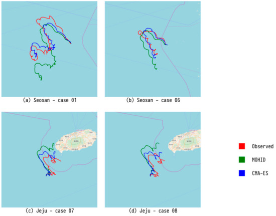
Figure 8. Comparison of trajectory predicted by our CMA-ES model, trajectory predicted by an existing numerical model (MOHID), and observed trajectory for four major drifters.

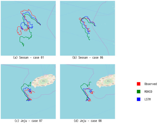
Figure 9. Comparison of trajectory predicted by our LSTM model, trajectory predicted by an existing numerical model (MOHID), and observed trajectory for four major drifters.

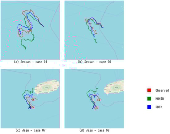
Figure 10. Comparison of trajectory predicted by our RBFN model, trajectory predicted by an existing numerical model (MOHID), and observed trajectory for four major drifters.

Except for the RNN series (RNN and LSTM), only the data at that point were used to predict the trajectory of a drifter at a point in hourly time. However, there is a difference in that RNN uses hidden layer neurons, which were used for prediction in previous instances, and LSTM showed the best performance as a measure of NCLS. It is believed that this is because the RNN series take into account the inertia of the drifter.

6. Conclusions

We extended and improved our previous study [8] which predicted the trajectories of drifters using evolutionary computation, and we also predicted the trajectories of drifters using various machine learning techniques [44,45,46,47,48,49]. To the best of the authors’ knowledge, this was the first trial in which machine learning has been applied to the prediction of drifter trajectories, and it significantly improved upon the representative numerical model, MOHID.

In terms of MAE, RBFN using the WEKA library showed the best performance, an improvement of 35.20% over the numerical model MOHID. LSTM using PyTorch showed the best performance regarding NCLS, an improvement of 6.24% over MOHID. These neural network-based methods did not take a long time to construct a model. In the future, we plan to experiment with other representative variants of RNNs such as gated recurrent units [50], and we will design more models that increase the performance of DNNs or basic RNNs by adding more training data.

References

- Nasello, C.; Armenio, V. A New Small Drifter for Shallow Water Basins: Application to the Study of Surface Currents in the Muggia Bay (Italy). J. Sens. 2016, 2016, 1–5. [Google Scholar] [CrossRef]
- Sayol, J.M.; Orfila, A.; Simarro, G.; Conti, D.; Renault, L.; Molcard, A. A Lagrangian model for tracking surface spills and SaR operations in the ocean. Environ. Model. Softw. 2014, 52, 74–82. [Google Scholar] [CrossRef]
- Sorgente, R.; Tedesco, C.; Pessini, F.; De Dominicis, M.; Gerin, R.; Olita, A.; Fazioli, L.; Di Maio, A.; Ribotti, A. Forecast of drifter trajectories using a Rapid Environmental Assessment based on CTD observations. Deep Sea Res. II Top. Stud. Oceanogr. 2016, 133, 39–53. [Google Scholar] [CrossRef]
- Zhang, W.-N.; Huang, H.-M.; Wang, Y.-G.; Chen, D.-K.; Zhang, L. Mechanistic drifting forecast model for a small semi-submersible drifter under tide–wind–wave conditions. China Ocean Eng. 2018, 32, 99–109. [Google Scholar] [CrossRef]
- De Dominicis, M.; Pinardi, N.; Zodiatis, G.; Archetti, R. MEDSLIK-II, a Lagrangian marine surface oil spill model for short-term forecasting—Part 2: Numerical simulations and validation. Geosci. Model Dev. 2013, 6, 1999–2043. [Google Scholar] [CrossRef]
- Miranda, R.; Braunschweig, F.; Leitao, P.; Neves, R.; Martins, F.; Santos, A. MOHID 2000—A coastal integrated object oriented model. WIT Trans. Ecol. Environ. 2000, 40, 1–9. [Google Scholar]
- Beegle-Krause, J. General NOAA oil modeling environment (GNOME): A new spill trajectory model. Int. Oil Spill Conf. 2001, 2001, 865–871. [Google Scholar] [CrossRef]
- Nam, Y.-W.; Kim, Y.-H. Prediction of drifter trajectory using evolutionary computation. Discrete Dyn. Nat. Soc. 2018, 2018, 1–15. [Google Scholar] [CrossRef]
- Lee, C.-J.; Kim, G.-D.; Kim, Y.-H. Performance comparison of machine learning based on neural networks and statistical methods for prediction of drifter movement. J. Korea Converg. Soc. 2017, 8, 45–52. (In Korean) [Google Scholar]
- Lee, C.-J.; Kim, Y.-H. Ensemble design of machine learning techniques: Experimental verification by prediction of drifter trajectory. Asia-Pac. J. Multimed. Serv. Converg. Art Humanit. Sociol. 2018, 8, 57–67. (In Korean) [Google Scholar]
- Özgökmen, T.M.; Piterbarg, L.I.; Mariano, A.J.; Ryan, E.H. Predictability of drifter trajectories in the tropical Pacific Ocean. J. Phys. Oceanogr. 2001, 31, 2691–2720. [Google Scholar] [CrossRef]
- Belore, R.; Buist, I. Sensitivity of oil fate model predictions to oil property inputs. In Proceedings of the Arctic and Marine Oilspill Program Technical Seminar, Vancouver, BC, Canada, 8–10 June 1994. [Google Scholar]
- Lehr, W.; Jones, R.; Evans, M.; Simecek-Beatty, D.; Overstreet, R. Revisions of the adios oil spill model. Environ. Model. Softw. 2002, 17, 189–197. [Google Scholar] [CrossRef]
- Berry, A.; Dabrowski, T.; Lyons, K. The oil spill model OILTRANS and its application to the Celtic Sea. Mar. Pollut. Bull. 2012, 64, 2489–2501. [Google Scholar] [CrossRef] [PubMed]
- Applied Science Associates. OILMAP for Windows (Technical Manual); ASA Inc.: Narrangansett, RI, USA, 1997. [Google Scholar]
- Reed, M.; Singsaas, I.; Daling, P.S.; Faksnes, L.-G.; Brakstad, O.G.; Hetland, B.A.; Hofatad, J.N. Modeling the water-accommodated fraction in OSCAR2000. Int. Oil Spill Conf. 2001, 2001, 1083–1091. [Google Scholar] [CrossRef]
- Al-Rabeh, A.; Lardner, R.; Gunay, N. Gulfspill Version 2.0: A software package for oil spills in the Arabian Gulf. Environ. Model. Softw. 2000, 15, 425–442. [Google Scholar] [CrossRef]
- Pierre, D. Operational forecasting of oil spill drift at Meétéo-France. Spill Sci. Technol. Bull. 1996, 3, 53–64. [Google Scholar] [CrossRef]
- Annika, P.; George, T.; George, P.; Konstantinos, N.; Costas, D.; Koutitas, C. The Poseidon operational tool for the prediction of floating pollutant transport. Mar. Pollut. Bull. 2001, 43, 270–278. [Google Scholar] [CrossRef]
- Zodiatis, G.; Lardner, R.; Solovyov, D.; Panayidou, X.; De Dominicis, M. Predictions for oil slicks detected from satellite images using MyOcean forecasting data. Ocean Sci. 2012, 8, 1105–1115. [Google Scholar] [CrossRef]
- Hackett, B.; Breivik, Ø.; Wettre, C. Forecasting the drift of objects sand substances in the ocean. In Ocean Weather Forecasting: An Integrated View of Oceanography; Springer: Dordrecht, The Netherlands, 2006. [Google Scholar]
- Breivik, Ø.; Allen, A.A. An operational search and rescue model for the Norwegian Sea and the North Sea. J. Mar. Syst. 2008, 69, 99–113. [Google Scholar] [CrossRef]
- Broström, G.; Carrasco, A.; Hole, L.; Dick, S.; Janssen, F.; Mattsson, J.; Berger, S. Usefulness of high resolution coastal models for operational oil spill forecast: The Full City accident. Ocean Sci. Discuss. 2011, 8, 1467–1504. [Google Scholar] [CrossRef]
- Ambjörn, C.; Liungman, O.; Mattsson, J.; Håkansson, B. Seatrack Web: The HELCOM tool for oil spill prediction and identification of illegal polluters. In Oil Pollution in the Baltic Sea; The Handbook of Environmental Chemistry; Springer: Berlin/Heidelberg, Germany, 2011; Volume 27, pp. 155–183. [Google Scholar]
- Aksamit, N.O.; Sapsis, T.; Haller, G. Machine-Learning Mesoscale and Submesoscale Surface Dynamics from Lagrangian Ocean Drifter Trajectories. J. Phys. Oceanogr. 2020, 50, 1179–1196. [Google Scholar] [CrossRef]
- Haller, G.; Sapsis, T. Where do inertial particles go in fluid flows? Phys. D Nonlinear Phenom. 2008, 237, 573–583. [Google Scholar] [CrossRef]
- Chorin, A.J. Numerical Solution of the Navier-Stokes Equations. Math. Comput. 1968, 22, 745–762. [Google Scholar] [CrossRef]
- Price, K.; Storn, R.M.; Lampinen, J.A. Differential Evolution: A Practical Approach to Global Optimization; Springer: Berlin/Heidelberg, Germany, 2006. [Google Scholar]
- Kennedy, J.; Eberhart, R. Particle swarm optimization. In Proceedings of the ICNN’95—International Conference on Neural Networks, Perth, Australia, 27 November–1 December 1995. [Google Scholar]
- Hansen, N.; Müller, S.D.; Koumoutsakos, P. Reducing the time complexity of the derandomized evolution strategy with covariance matrix adaptation (CMA-ES). Evol. Comput. 2003, 11, 1–18. [Google Scholar] [CrossRef]
- Boser, B.E.; Guyon, I.M.; Vapnik, V.N. A Training Algorithm for Optimal Margin Classifiers. In Proceedings of the 5th Annual ACM Workshop on Computational Learning Theory, New York, NY, USA, 27–29 July 1992; pp. 144–152. [Google Scholar]
- Drucker, H.; Burges, C.J.; Kaufman, L.; Smola, A.J.; Vapnik, V. Support vector regression machines. In Proceedings of the Advances in Neural Information Processing Systems, Denver, CO, USA, 1–6 December 1997. [Google Scholar]
- Koza, J.R. Genetic Programming: On the Programming of Computers by Means of Natural Selection; MIT Press: Cambridge, MA, USA, 1992. [Google Scholar]
- Moody, J.; Darken, C.J. Fast Learning in networks of locally-tuned processing units. Neural Comput. 1989, 1, 281–294. [Google Scholar] [CrossRef]
- Nair, V.; Hinton, G.E. Rectified linear units improve restricted Boltzmann machines. In Proceedings of the 27th International Conference on Machine Learning (ICML), Haifa, Israel, 21–24 June 2010; pp. 807–814. [Google Scholar]
- Srivastava, N.; Hinton, G.; Krizhevsky, A.; Sutskever, I.; Salakhutdinov, R. Dropout: A simple way to prevent neural networks from overfitting. J. Mach. Learn. Res. 2014, 15, 1929–1958. [Google Scholar]
- Hochreiter, S. The Vanishing Gradient Problem During Learning Recurrent Neural Nets and Problem Solutions. Int. J. Uncertain. Fuzziness Knowl. Based Syst. 1998, 6, 107–116. [Google Scholar] [CrossRef]
- Rumelhart, D.E.; Hinton, G.E.; Williams, R.J. Learning representations by back-propagating errors. Nature 1986, 323, 533–536. [Google Scholar] [CrossRef]
- Hochreiter, S.; Schmidhuber, J. Long short-term memory. Neural Comput. 1997, 9, 1735–1780. [Google Scholar] [CrossRef]
- Frank, E.; Hall, M.; Trigg, L. Weka 3: Data Mining Software in Java; The University of Waikato: Hamilton, New Zealand, 2006. [Google Scholar]
- Ketkar, N. Introduction to PyTorch. In Deep Learning with Python; Apress: Berkeley, CA, USA, 2017; pp. 195–208. [Google Scholar]
- Breiman, L. Bagging predictors. Mach. Learn. 1996, 24, 123–140. [Google Scholar] [CrossRef]
- Golik, P.; Doetsch, P.; Ney, H. Cross-entropy vs. squared error training: A theoretical and experimental comparison. In Proceedings of the 14th Annual Conference of the International Speech Communication Association (Interspeech 2013), Lyon, France, 25–29 August 2013; pp. 1756–1760. [Google Scholar]
- Seo, J.-H.; Lee, Y.H.; Kim, Y.-H. Feature Selection for Very Short-Term Heavy Rainfall Prediction Using Evolutionary Computation. Adv. Meteorol. 2014, 2014, 1–15. [Google Scholar] [CrossRef]
- Kim, Y.-H.; Moon, S.-H.; Yoon, Y. Detection of Precipitation and Fog Using Machine Learning on Backscatter Data from Lidar Ceilometer. Appl. Sci. 2020, 10, 6452. [Google Scholar] [CrossRef]
- Moon, S.-H.; Kim, Y.-H. Forecasting lightning around the Korean Peninsula by postprocessing ECMWF data using SVMs and undersampling. Atmos. Res. 2020, 243, 105026. [Google Scholar] [CrossRef]
- Moon, S.-H.; Kim, Y.-H. An improved forecast of precipitation type using correlation-based feature selection and multinomial logistic regression. Atmos. Res. 2020, 240, 104928. [Google Scholar] [CrossRef]
- Moon, S.-H.; Kim, Y.-H.; Lee, Y.H.; Moon, B.-R. Application of machine learning to an early warning system for very short-term heavy rainfall. J. Hydrol. 2019, 568, 1042–1054. [Google Scholar] [CrossRef]
- Kim, H.-J.; Park, S.M.; Choi, B.J.; Moon, S.-H.; Kim, Y.-H. Spatiotemporal Approaches for Quality Control and Error Correction of Atmospheric Data through Machine Learning. Comput. Intell. Neurosci. 2020, 2020, 1–12. [Google Scholar] [CrossRef]
- Chung, J.; Gulcehre, C.; Cho, K.; Bengio, Y. Empirical evaluation of gated recurrent neural networks on sequence modeling. arXiv 2014, arXiv:1412.3555. [Google Scholar]
Publisher’s Note: MDPI stays neutral with regard to jurisdictional claims in published maps and institutional affiliations. |
© 2020 by the authors. Licensee MDPI, Basel, Switzerland. This article is an open access article distributed under the terms and conditions of the Creative Commons Attribution (CC BY) license (http://creativecommons.org/licenses/by/4.0/).