Dynamic All-Red Signal Control Based on Deep Neural Network Considering Red Light Runner Characteristics

Abstract

Despite recent advances in technologies for intelligent transportation systems, the safety of intersection traffic is still threatened by traffic signal violation, called the Red Light Runner (RLR). The conventional approach to ensure the intersection safety under the threat of an RLR is to extend the length of the all-red signal when an RLR is detected. Therefore, the selection of all-red signal length is an important factor for intersection safety as well as traffic efficiency. In this paper, for better safety and efficiency of intersection traffic, we propose a framework for dynamic all-red signal control that adjusts the length of all-red signal time according to the driving characteristics of the detected RLR. In this work, we define RLRs into four different classes based on the clustering results using the Dynamic Time Wrapping (DTW) and the Hierarchical Clustering Analysis (HCA). The proposed system uses a Multi-Channel Deep Convolutional Neural Network (MC-DCNN) for online detection of RLR and also classification of RLR class. For dynamic all-red signal control, the proposed system uses a multi-level regression model to estimate the necessary all-red signal extension time more accurately and hence improves the overall intersection traffic safety as well as efficiency.

1. Introduction

As the traffic volume in urban areas has increased significantly over the last decades, there has been many demands and efforts to develop and deploy technologies for intelligent transportation systems in order to address issues of traffic congestion, safety, efficiency, and also environmental improvements [1]. Undoubtedly, one of the most complex, dangerous, and important traffic environments on the road is the intersection, where traffic flows from different directions overlap in a common space, and it also has substantial impacts on the overall urban traffic efficiency and safety [2]. At intersections, traffic flows from different directions are typically coordinated through traffic light systems to prevent conflicting traffic flows passing the intersection simultaneously. Therefore, if a traffic participant violates the traffic rules imposed by the traffic light, the other participants in the intersection inevitably face the risk of an accident. The most representative example of such a traffic participant that violates the traffic signal is the Red Light Runner (RLR) [3].

An RLR is a vehicle passing through an intersection, ignoring the traffic signal when the traffic light is red. According to the AAA Foundation for Traffic Safety, the number of deaths from RLRs increased by 31% from 2009 to 2017. In addition, the Insurance Institute for Highway Safety (IIHS) reported in 2017 that approximately 132,000 casualties were caused by the RLR. Also, the Manual on Uniform Traffic Control Devices (MUTCD), a standard for maintaining and installing traffic control devices, provides the control of intersection signals to reduce RLR accidents [4]. In general, intersection traffic lights consist of green, yellow, red and all-red signals. All-red signals exist when the intersection traffic light changes from yellow to red and red to green, and is used to prevent accidents caused by vehicles entering the intersection with the yellow signal [5]. MUTCD proposes the construction of a system that extends the all-red signal of intersection traffic lights when an RLR is detected. The length of the all-red signal needs to be determined so that collision by RLR does not occur in the intersection. One of the methods of determining the signal extension time is to use a statistical method to extend a constant time regardless of the current state of the vehicle. Another method extends the all-red signal by dividing the distance to the collision prediction point by the speed of the current vehicle.

The current all-red signal extension system depends only on the vehicle speed at the moment when an RLR is detected. However, if the RLR does not move at a fixed speed as expected, the safety in the intersection cannot be ensured. Therefore, in this paper, we propose a framework for a dynamic all-red signal control system that determines the signal extension time according to the driving pattern of the detected RLR. In this proposed system, driving patterns of RLR vehicles are distinguished through the Multi-Channel Deep Convolutional Neural Network (MC-DCNN) [6]. Also, a multi-level regression strategy, consisting of the Hougen–Watson nonlinear regression model [7] and a quadratic polynomial regression model, is used to estimate the necessary all-red signal extension time with improved accuracy.

The structure of the paper is organized as follows. Section 2 introduces conventional RLR prediction and signal extension methodologies. An overview of the proposed system is presented in Section 3. Clustering and classification based on the characteristics of RLRs are covered in Section 4. The proposed dynamic signal control model is described in Section 5. We validate the performance of the proposed system in Section 6 and Section 7. Finally, conclusions are discussed in Section 8.

2. Related Works

RLR is an action that threatens the traffic system passing through by ignoring the signaling system at a signaled intersection. RLR is a serious problem that can lead to fatal traffic accidents as well as minor traffic violations. A collision between a violating vehicle and another vehicle legally passing through an intersection and a green traffic light is called an RLR collision. To avoid RLR-related collisions, it is important to identify factors that have a significant impact on the behavior of RLR drivers and to predict RLR likelihood in real-time [8].

Li et al. [9] proposed a connected vehicle based dynamic all-red extension (DARE) framework to prevent potential collisions due to RLR. The proposed method performs binary classification of RLR and Non-RLR based on non-weighted and weighted least square support vector machines (LS-SVM) using continuous trajectories measured by radar sensors. As a result, RLR and Non-RLR were classified with higher accuracy compared to other techniques based on conventional inductive loop detection. In [10], RLR prediction consists of two parts: arrival time and vehicle behaviors when the vehicle reaches the stop line. The proposed technique is a Bayesian network (BN) probability model based on continuous trajectories collected by radar sensors for RLR prediction. Based on the vehicle’s speed, acceleration, and car-following behavior, and the causality of BN, RLR prediction performance was improved. In addition, the driving decision maker was provided with the predicted RLR probability and contributed to the improvement of traffic safety. de Goma et al. [11] proposed a camera-based RLR detection technique using a Single Shot Detector (SSD). In this study, researchers use cameras to collect data at intersections. The proposed system achieved RLR detection performance of 92.1% by applying a deep learning based approach. However, despite the high detection performance, the proposed technique focused on detection rather than the prediction of RLR as a camera-based technique. In [12], a random forest-based learning model was proposed to predict RLR violation. In addition, observation data and driver simulator data were used to analyze factors affecting RLR. According to the results of the proposed prediction model, the important factors for predicting RLR violations are the distance between the vehicle and the intersection, time to intersection (TTI) and the speed of the vehicle at the yellow onset.

In order to reduce accidents at intersections, techniques to control the traffic signal when RLR is detected has been proposed. In [13], a traffic signal countdown (CT) auxiliary device is used in order to reduce the RLR. The CT-based traffic light system aims to reduce RLR by providing the driver with the remaining time of green light. However, at the end of the green light’s duration, the RLR may increase as the driver accelerates through the intersection before the signal changes. Likewise, if there is little red light remaining when reaching the intersection, the driver will not decelerate and may enter the intersection early and an RLR may occur. Control of the yellow signal interval had a positive effect on the reduction of RLR [14]. Control of the yellow signal interval helped the driver to make a driving decision at the intersection. According to the study, the time duration of the yellow signal that most effectively reduces RLR is 5 s, and when the duration of the yellow signal exceeds 5 s, RLR is increased again. Since this method is a fixed yellow signal setting, the effect is reduced if the driver gets used to the yellow signal in the long term. Retting et al. [15] proposed an extension of the yellow signal and an enforcement system using a Red Light Camera (RLC). The incidence of RLR was reduced by 36% by increasing the duration of the yellow stop light by 1 s. In addition, by applying an enforcement system using RLC, the RLR incidence rate was reduced by more than 96%. Collotta et al. [16] proposed a method to reduce RLR violations by dynamically allocating signal periods through a Wireless Sensor Network (WSN). The main goal is to dynamically change the green time based on the queue length, allocating a larger green time to the road with the longest queue. Experiments conducted in Philadelphia reduced RLR violations through dynamic assignment of traffic signal periods. However, changing signal settings under the influence of RLR can lead to an asymmetric traffic assignment problem. In [17], authors argued that two distinct problems can be formulated to address the asymmetric traffic assignment problem: First, the global optimization of signal setting and traffic assignment (GOSSTA) combined problem and second, the local optimization of signal setting and traffic assignment (LOSSTA) combined problem. Related to these problems, Adacher et al. [18] transformed the GOSSTA problem into a surrogate continuous optimization problem via a generalized surrogate problem methodology based on an online control scheme and solved the latter using a standard gradient-based approach. On the other hand, D’Acierno et al. [19] proposed an Ant Colony Optimization (ACO) algorithm to solve LOSSTA. The results of the proposed ACO algorithm for real networks were able to get the solution in a shorter time with the same accuracy as the conventional method of the successive averages (MSA) approach [20].

Kashani et al. [21] identified driver and vehicle characteristics that affect accidents using classification and regression tree techniques based on the 2012–2016 Isfahan crash database. In this study, the tree model divided drivers into three age groups: under 22.5 years old, 22.5 to 51.5 years old, and over 51.5 years old. It also suggested improving driver education, increasing traffic fines, and banning drivers with poor driving history to reduce RLR. Fu et al. [22] proposed a step-by-step penalty strategy to prevent the re-offending of RLR vehicles. Despite the rigorous penalty strategy to reduce RLR, its effectiveness was limited. The reason is that traffic delays for other vehicles due to the potential risk of collision with RLR vehicles are not included. In addition, both unintentional and intentional RLRs are subject to the same penalties because the proposed system cannot make a clear distinction between unintentional RLR and intentional RLR. This may be unfair for unintended RLR violators.

Conventional studies have focused on the binary classification of RLR and Non-RLR, and the extension of fixed time signals. Penalties were also effective in reducing RLR. Additionally, some studies have discussed penalty policies to reduce RLR. However, excessive penalties for unintended RLR are a problem to be solved. Our proposed system performs a specific classification of RLR based on features rather than binary classification of RLR and Non-RLR. This can contribute to the classification of unintended RLRs based on the characteristics of RLRs, and is expected to positively help in constructing a stronger RLR fines system. In addition, our proposed system can contribute to the improvement of safety and efficiency of the intersection traffic system based on the dynamic all-red signal extension conforming to the specified RLR class. As discussed above, while it is still possible that the proposed dynamic all-red signal extension may cause an asymmetric traffic assignment problem, it is not the primary focus of this paper to improve the overall traffic efficiency by solving the asymmetric traffic assignment problem as done in many aforementioned related works. Instead, we focus more on improving the safety of intersection traffic by preventing accidents due to RLRs and also the efficiency of it by overcoming the problem of conventional fixed signal extension mechanisms.

3. System Overview

For better intersection safety, a dynamic all-red signal control is necessary to avoid collisions due to sudden appearances of RLRs. To address the issues with conventional fixed signal extension approach, the proposed system identifies first which incoming vehicles are likely to be RLRs and then utilizes the driving characteristics of the detected RLR to adjust the length of the all-red signal accordingly. Hence, the proposed system improves the overall safety as well as efficiency of intersection traffic.

Figure 1 shows the overall architecture of the proposed dynamic all-red signal control system. The first step of the process begins with traffic data collection from the intersection traffic environment. Traffic data to be collected includes traffic signal as well as all incoming vehicles’ movement data such as each vehicle’s speed, acceleration, distance to the intersection (DTI) and headway during a certain time duration. Note that, for the purpose of all-red signal length control, the system requires traffic data measured while the traffic signal is in the yellow state. The next step of the process is to identify which incoming vehicles are likely to be RLR. As shown in Figure 1, we use the MC-DCNN classifier for this purpose. The proposed MC-DCNN classifier classifies not only whether an incoming vehicle is likely to be an RLR or not but it also classifies into several different types of RLR based on the vehicle’s driving characteristics if the vehicle is likely to be an RLR. Then the last step of the process is to determine the length of all-red signal extension based on the detailed classification result from the MC-DCNN. For this step, we use a multi-level regression approach consisting of the Hougen–Watson nonlinear regression and a quadratic polynomial fitting to determine the necessary all-red signal extension time. More details on each of the steps in the process are covered in the following sections.

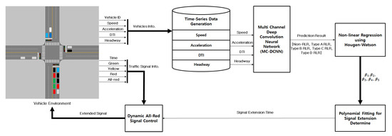
Figure 1. The proposed dynamic all-red signal control architecture.

4. Clustering and Classification

In general, the intersection is considered as the most complex road traffic environment. Furthermore, each vehicle on the road shows very different driving characteristics depending on the driving style or physical/mental conditions of the driver in the vehicle. Hence, the movements of vehicles approaching an intersection to cross are very different from each other and are affected by various factors. Thus, for safer intersection traffic through traffic light control, it is not enough to identify which vehicle is likely to be an RLR. To determine the length of the all-red signal appropriately, it is also necessary to identify the characteristics of the vehicle movement and determine the necessary all-red signal time for the vehicle accordingly. Our approach to addressing this issue is to utilize techniques for time-series clustering for characterization of RLRs into several clusters according to their movements. Then, the identified groups of clusters are used as labels for the generation of the traffic dataset to be used for training the MC-DCNN classifier.

Figure 2 shows the overall procedure for dataset generation. The data collected from the traffic environment includes traffic signal data, vehicle movement data, and also whether each vehicle is RLR or non-RLR. In the collected raw traffic data, RLR vehicles are not distinguished according to their characteristics. Therefore, clusters for each RLR characteristic are generated through Dynamic Time Wrapping (DTW) and Hierarchical Clustering Analysis (HCA) processes. After this process, a dataset for training MC-DCNN is constructed based on the traffic data together with RLR cluster labels so that each vehicle in the dataset is now labeled with a cluster ID according to its driving characteristics.

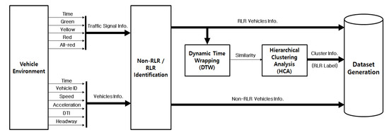
Figure 2. Dataset preparation process for classification.

4.1. Time-Series Clustering

Conventional studies are based on the assumption that the RLR passes through the intersection at a fixed speed. However, RLR vehicles have a variety of driving characteristics in the real world. Therefore, we adopt the clustering method to define the driving characteristics of RLR. The clustering method performs merging into one group when the similarity between data is high, and splits into another group when the similarity is low. However, driving characteristics are difficult to define with one moment of data. Therefore, driving data continuously measured over a certain period of time and a clustering method for time-series data are required. In general, the time-series clustering method consists of a representation of continuous-time trajectories in time-series form, calculation of similarity or distance measure between every pair of time-series data, and then clustering all time-series data into several groups according to the similarity measure.

At an intersection, a vehicle’s speed profile changes dramatically in response to traffic signals. Vehicles with no intention of signal violations and RLR vehicles typically show different movement from the start of the yellow signal [23]. Furthermore, it is well known that the speed profile of a vehicle represents the driving pattern of the vehicle and also reflects various factors affecting the vehicle motion such as driving condition and driving style [24,25]. As an illustration of how other factors affect the speed profile of a vehicle, Figure 3 shows a comparison between driving profiles of two different RLR clusters. Figure 3a shows a pattern in which the speed and acceleration are maintained without significant change after 1 s of yellow onset. The DTI shows a decreasing pattern because it is moving toward the intersection. The headway has a value of 1, which means that there is no preceding vehicle. On the other hand, the headway shown in Figure 3b changes from 1 to 0 around 1.5 s after the yellow onset. This means that a preceding vehicle suddenly appeared in front of the vehicle from the other lane. With its influence, the speed and acceleration of the RLR decreases rapidly and then increases as the headway increases again.

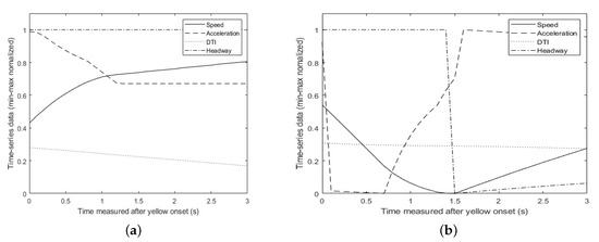
Figure 3. Comparison of driving profiles from two different Red Light Runner (RLR) clusters. (a) Speed maintenance pattern; (b) Acceleration after deceleration by the preceding vehicle pattern.

Similarity measure is a way to check the similarity between time-series data. We calculate the similarity measure based on the speed profile of each vehicle and utilize it to create a cluster as the speed profile of a vehicle is one of the representative time-series data used to distinguish RLR vehicles. The most commonly used methods for calculating the similarity measure are the Euclidian distance and DTW. Euclidian distance is a technique to calculate the distance between two time-series in each time slice by one-to-one matching. This technique is simple and fast, but there is a limitation when there exists a time shift between sequences. In comparison, DTW performs one-to-many or many-to-one matching and is more robust than the Euclidian distance technique for time shifts between sequences [26]. Therefore, we use DTW to calculate the similarity measure in the speed profiles of various vehicles.

Once the similarity measures are calculated through DTW, clustering is performed through Hierarchical Clustering Analysis (HCA) [27]. HCA is an algorithm that performs clustering using a hierarchical tree structure. Since the number of clusters of driving characteristics of RLR cannot be pre-defined easily, we determine the number of clusters by investigating the tree structure where the difference in similarity measure calculated by DTW increases rapidly. Through the HCA process, the driving characteristics of RLR vehicles are divided into four groups which are (i) acceleration (Type A RLR), (ii) acceleration after deceleration (Type B RLR), (iii) speed maintenance (Type C RLR), and (iv) acceleration after deceleration by preceding vehicle (Type D RLR). Here, the created clusters are used for the training process of the classification model.

4.2. Classification

A traditional technique for RLR detection and classification is the Support Vector Machine (SVM) [28,29]. SVM is a technique that classifies into two classes by obtaining a decision boundary that separates several sample points. The decision boundary separates two classes of clusters, and the sample closest to the boundary becomes the support vector. SVM classifies the binary classes by finding the decision boundary that maximizes the margin between the support vector and the decision boundary. Multi-class SVM for multi-class classification obtains sub-SVMs for classifying each class, and performs multi-class classification based on this idea [30,31]. Recently, deep learning models with higher classification accuracy than SVM have been proposed [32]. A representative deep learning model is the Convolutional Neural Network (CNN). In general, CNN consists of a convolutional layer, Rectified Linear Unit (ReLU) layer, pooling layer, and fully-connected layer [33]. The convolutional layer extracts the features of the input, while the ReLU layer increases the non-linearity properties of the convolutional layer. The pooling layer prevents overfitting through down-sampling. Finally, scores are calculated for each class of output in the fully connected layer. However, the general CNN is an image-based model but not for the time-series data. Therefore, a deep learning model using time-series data as input is needed.

We use the Multi-Channel Deep Convolutional Neural Network (MC-DCNN), a signal data-based model for time-series classification [34,35]. MC-DCNN is a model that uses time-series data of each sensor as the input of multi-channels. The proposed MC-DCNN model uses the speed, acceleration, headway, and DTI as input signals. Since the driving pattern obtained from the speed profile of the vehicle is affected by various driving conditions, the headway and DTI are also selected as inputs to consider the front vehicle and the distance to the intersection. In addition, speed and acceleration are selected to analyze the driving pattern of the RLR. Since the input signal used for MC-DCNN is time-series data, a window length and a prediction time after yellow onset are also required to determine the time interval of traffic data measurement and also to determine when to perform the classification. Prediction time after yellow initiation refers to the point at which RLR is predicted after the start of the yellow signal. If the window length is 2 s and the prediction time after the onset of yellow is 3 s, 2 s of data are collected from 1 to 3 s after the yellow onset.

The proposed network structure consists of two convolutional, ReLU, pooling layers and the last fully connected layer. The convolution layer is composed of a 1D convolution because the driving pattern is identified through the feature over time [36]. The last layer is a softmax, which outputs a distribution over classes. The classes are defined in five categories: Non-RLR, Type A RLR, Type B RLR, Type C RLR, and Type D RLR.

5. Dynamic All-Red Signal Control

In order to dynamically control the length of the all-red signal considering the driving characteristics of RLRs, it is necessary to predict the time at which the RLR under consideration can completely pass the intersection. For this purpose, we use multi-level regression to predict the necessary time duration for the RLR to completely get out of the intersection from the moment of prediction, which we call the intersection passing time in the sequel. The input data for the regression model is composed of the speed, DTI, and headway of the RLR at the prediction time. As the first level of regression for prediction, we use the Hougen–Watson model in (1), one of the nonlinear regression models, to roughly estimate the intersection passing time.

$$\widehat{y}=\frac{{\beta }_1{x}_2-x_3/{\beta }_5}{1+{\beta }_2{x}_1+{\beta }_3{x}_2+{\beta }_4{x}_3}$$

(1)

where $\widehat{y}$ is the predicted intersection passing time and variables $x_1,x_2,x_3$ are the DTI, the speed, the headway of a vehicle, respectively. ${\beta }_1$, ⋯, ${\beta }_5$ in (1) are parameters to be determined through regression using data. In our study, we determined these parameters by the Levenberg–Marquardt nonlinear least squares algorithm [37,38]. The Levenberg–Marquardt algorithm is a combination of two minimization methods, which are known as gradient descent and Gauss–Newton. The Levenberg–Marquardt operates in a gradient descent method when it is far from the solution, and finds the solution in a Gauss–Newton method near the solution. In addition, the Levenberg–Marquardt method is more stable than the Gauss–Newton method and converges to the solution relatively quickly, so the Levenberg–Marquardt method is mostly used in the nonlinear least square problem. The Levenberg–Marquardt nonlinear least squares algorithm optimizes the model by iteratively reducing the sum of squares of errors between the model and the measured data through an update process to the parameters.

As the prediction of intersection passing time of RLR through the Hougen–Watson model is a rough estimate of actual intersection passing time required for the RLR, the predicted time can be much shorter than necessary for some cases. This means that if the length of all-red signal is adjusted according to this estimated intersection passing time, then vehicles from other direction may enter the intersection before the RLR completely clears the intersection. Thus, it is necessary to address such safety issue caused by using only the Hough–Watson model in predicting intersection passing time. For this purpose, we also use the quadratic polynomial fitting model as the second level of regression based on the prediction results of the Hougen–Watson model for better safety of intersection traffic. Furthermore, since prediction of the intersection passing time of RLR without considering the driving characteristics of the RLR, the predicted intersection passing time can be too conservative in some cases. Therefore, to address this issue and improve the overall traffic efficiency, we build separate multi-level regression models according to RLR classes, as described in Section 4.2, and predict the intersection passing time of an RLR according to its RLR class. More details on this multi-level regression framework and results are given in Section 7.3.

6. Traffic Simulation

The system proposed in this paper requires data collection for clustering and classification. However, it is difficult to collect traffic data in a real environment. Therefore, we use the Vissim traffic simulator, which is widely used in transportation engineering for microscopic traffic simulation, to collect intersection traffic data and also to evaluate the performance of the proposed system.

Figure 4 shows the intersection traffic environment configured in Vissim and also shows the traffic signal phases. A standard intersection model is used, which has three input lanes and two output lanes for each ramp way. The leftmost input lane is for left turning, and the center lane is for straight traffic. The far right lane is used for both straight and also for right turning with 20% probability. The traffic signal cycle at the intersection consists of four phases. The signal duration is set to be 27 s for straight traffic and 15 s for left turning traffic according to the traditional Webster’s method [39]. On the other hand, the signal duration for yellow and red in each phase are set differently according to the traffic speed based on the FHWA’s Traffic Signal Timing Manual [40]. Traffic flow includes car-following and lane change motion.

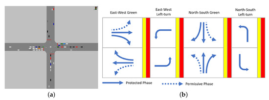
Figure 4. Intersection traffic simulation in Vissim. (a) Simulated intersection traffic; (b) Traffic signal phase.

Since Vissim provides two different models, called the continuous decision model and one decision model, to mimic the reaction patterns of real drivers at an intersection when the traffic signal changes from green to yellow, we utilize both of these models in our simulations to generate a more realistic intersection traffic data.

In a continuous decision model, there are two options available. First, a vehicle will not brake, if even the maximum deceleration would not allow for a stop at the stop line. Second, a vehicle brakes if a vehicle cannot pass the traffic light within 2 s when continuing at its current speed rate. On the other hand, in one decision model, the decision made at the time of the yellow onset is kept until the vehicle has passed the stop line. A vehicle stops according to the following probability

$$p=\frac{1}{1+e^{-{\alpha }_1-{\alpha }_{2}v-{\alpha }_{3}dx}}$$

(2)

where v is the vehicle’s current speed, $dx$ is the DTI, and ${\alpha }_1$, ${\alpha }_2$, ${\alpha }_3$ are fitting parameters. In our simulation, we use the default values for these fitting parameters, which are ${\alpha }_1=1.59$, ${\alpha }_2=0.27$, and ${\alpha }_3=-0.26$ provided in Vissim.

Figure 5 shows representative reaction patterns of traffic observed in simulation according to two decision models. Depending on the state of a vehicle such as current speed, DTI at the time of yellow onset, the vehicle reacts into three different patterns. First, Go is the case when a vehicle enters the intersection before the red signal, Stop is the case when a vehicle stops at the stop line on the red signal, and finally, RLR means the case when a vehicle is entering the intersection at the red signal [9]. Figure 5a shows the change in speed for each reaction of continuous decision traffic. The vehicle with Go reaction does not have a red signal before the distance to the intersection becomes 0 m. The vehicle with Stop reaction stops gradually with a yellow signal starting at a distance more than 60 m from the intersection. However, vehicles with the RLR reaction show that they start to accelerate rapidly between about 15 to 20 m before the intersection. Figure 5b shows the speed change for each reaction of one decision model. In one decision model, Go and Stop reactions are similar to those in the continuous decision model. On the other hand, one of the vehicles with RLR reaction maintains speed without significant change in its speed even when the yellow signal starts. Thus, for the purpose of our study in this paper, we can confirm that the intersection traffic simulated in Vissim according to two decision models can provide a close enough representation to actual intersection traffic.

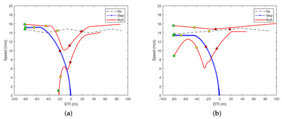
Figure 5. Comparison of vehicle reaction pattern between continuous decision model and one decision model where colored circles in the images indicate the traffic light signals. (a) Examples of velocity profiles with continuous decision model; (b) Examples of velocity profiles with one decision model.

Table 1 shows the statistical result of 2567 vehicle data (RLR: 1710 and non-RLR:857) collected over 24 h simulation in Vissim. This result is obtained with vehicles of which DTI is less than 100 m at the time of yellow onset. In the case of the continuous decision model, acceleration of RLR is relatively high compared to that of Non-RLR. This means that RLR vehicles attempt to pass the intersection faster than non-RLR vehicles. In the case of RLR in one decision model, acceleration is the lowest but it has a high headway on average. In addition, the mean and standard deviation of acceleration are the smallest and thus the movement of maintaining the speed is observed. In the results, we can also observe that RLR vehicles of the two decision models have higher mean speed than other reaction patterns. In addition, the mean of DTI in both decision models is farther than that with the Go reaction but closer than that of the Stop reaction.

Table 1. Statistical results of traffic simulation data collected at the time of yellow onset.

Variable	Decision Model	Behavior	Mean	Standard Deviation
		RLR	14.1337	1.5924
	Continuous	Go	13.6342	1.3388
Speed (m/s)		Stop	12.2642	4.4733
		RLR	15.2914	1.3388
	One	Go	13.8057	2.7491
		Stop	12.3939	4.3449
		RLR	0.3404	0.7978
	Continuous	Go	0.2910	0.6586
Acceleration (m/s2)		Stop	0.1817	0.8693
		RLR	-0.0500	0.4520
	One	Go	0.2076	0.5830
		Stop	0.1709	0.7996
		RLR	37.6579	3.7382
	Continuous	Go	16.0680	10.6932
DTI (m)		Stop	63.8649	21.3053
		RLR	51.3914	6.3918
	One	Go	19.1971	12.2729
		Stop	65.6994	21.5267
		RLR	88.8779	76.6408
	Continuous	Go	88.9833	81.1717
Headway (m)		Stop	86.4493	78.2994
		RLR	106.6986	77.8763
	One	Go	95.3744	83.9599
		Stop	89.2601	79.3263

7. Results

In this section, we present results of the proposed clustering, classification, and dynamic all-red signal control approach obtained through traffic simulations in Vissim.

7.1. Clustering

As described in Section 4.1, we use the DTW algorithm to measure the similarity between a pair of speed profile time-series. Figure 6 shows several examples of speed profile time-series data, selected from different clusters which are determined later through the HCA clustering process, to illustrate the effect of the DTW algorithm for optimal alignment of two time-series data and the similarity measure calculated between them. Figure 6a shows a comparison between speed profiles from Type A RLR and Type B RLR clusters. The similarity measure between these two time-series data, calculated as the accumulated pairwise Euclidean distance, is 131.26 in this case. Similarly, Figure 6b,c also show the similarity results from different RLR clusters where similarity measures calculated from the DTW algorithm are 87.85 and 71.23, respectively. On the other hand, Figure 6d shows the similarity result between a pair of speed profile time-series selected from the same cluster, which is Type B RLR in this case. For these speed profile time-series data, the similarity measure from the DTW algorithm is less than 25, which is substantially lower than the other three cases in the figure and hence clearly indicates that these two time-series are quite similar to each other in terms of their shapes while they may be in slightly different phases.

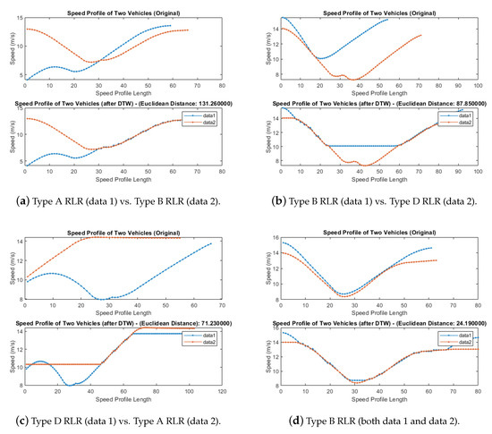
Figure 6. Examples of similarity results through the Dynamic Time Wrapping (DTW) algorithm.

Next, to determine the number of clusters via HCA based on the similarity measures, it is necessary to choose a threshold appropriately for the value of a similarity measure. If the threshold for cluster separation is too low, then there will be too many clusters formed and the driving characteristics of RLRs between clusters are not clearly distinguishable. Therefore, we investigate the hierarchical structure of clusters generated from HCA for all RLR traffic datasets and choose to separate clusters when the similarity measure suddenly increases more than 50 in the HCA process since clusters formed from this are most reasonably distinguishable in terms of their driving characteristics. As a result, there are four different clusters formed for RLRs, as described in Section 4.1.

Figure 7 shows the result of clustering generated through the HCA process for all RLR traffic data collected from the Vissim simulation. Figure 7a–d shows RLR speed profiles of each cluster. As shown in the figure, four RLR clusters show different driving characteristics where RLR in Type A keeps accelerating to cross an intersection, RLR in Type B first decelerates and then accelerates, RLR in Type C is mostly maintaining its speed, and finally, RLR in Type D exhibits similar behavior as Type B in the beginning but decelerates rapidly shortly after accelerating due to the sudden appearance of a proceeding vehicle in front of the RLR.

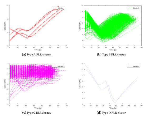
Figure 7. Clustering of RLR traffic dataset through Hierarchical Clustering Analysis (HCA).

7.2. Classification

For online classification of an incoming vehicle to predict whether the vehicle is a Non-RLR or one of the four RLR types, we use MC-DCNN as described in Section 4.2. For training of the MC-DCNN model, we built a training dataset from traffic data consisting of time-series of vehicle speed, acceleration, DTI, and headways with cluster type determined through HCA so that each vehicle in the training dataset is labeled whether it is a Non-RLR, Type A RLR, Type B RLR, Type C RLR, and Type D RLR. Therefore, as shown in Figure 1, the trained MC-DCNN model gives a prediction to which class out of the above five classes an incoming vehicle is classified.

To evaluate the classification performance MC-DCNN, we compare the classification accuracy of MC-DCNN with that of SVM using the validation dataset. Table 2 and Table 3 are classification accuracy results using SVM and MC-DCNN, respectively. In the results, the classification accuracy is 100% if the classifier classifies all five classes, Non-RLR, Type A, B, C, D RLR correctly. The “window size” means the time-series length of input data, and the “prediction time after yellow onset” means the time when a classifier performs classification after yellow onset. In the case of SVM, if the window size is 0 s (i.e., there is only one data point in the input time-series), the accuracy is lower than about 60% regardless of prediction time. Table 2 also shows that the longer the input time-series length, the better the classification performance. The highest accuracy appears when the window size is 3 s and the prediction time is 2.5 or 3 s after yellow onset.

Table 2. Classification accuracy of Support Vector Machine (SVM) classifier.

	Prediction Time after Yellow Onset (Sec)
		0	0.5	1	1.5	2	2.5	3
Window size (sec)	0	56.6%	57.5%	58.6%	57.1%	57.4%	57.7%	59%
	0.5	79.8%	85.4%	85%	85.2%	84.6%	85.4%	85.1%
	1	84.3%	86.5%	87.7%	87.2%	87%	87.3%	87.5%
	1.5	88.4%	88.6%	89%	90%	90.2%	90.3%	90%
	2	90.6%	92.2%	92.6%	93.3%	93.3%	93.4%	93.3%
	2.5	94%	94.7%	95.6%	95.9%	95.8%	95.8%	96%
	3	98.9%	98.9%	99.2%	99.3%	99.3%	99.4%	99.4%

Table 3. Classification accuracy of the Multi-Channel Deep Convolutional Neural Networks (MC-DCNN) classifier.

	Prediction Time after Yellow Onset (Sec)
		0	0.5	1	1.5	2	2.5	3
Window size (sec)	0	87.3%	92.5%	92.9%	90.7%	89.2%	95.4%	99.5%
	0.5	90.7%	95.2%	96.4%	97.4%	98.1%	98%	99.6%
	1	93.5%	96.4%	97.1%	97.8%	98.3%	98.4%	99.9%
	1.5	93.5%	96.9%	97.4%	98.4%	98.6%	99.1%	99.9%
	2	93.8%	96.2%	97.1%	99%	98.9%	99.3%	99.9%
	2.5	94.3%	96.7%	97.2%	98.7%	98.2%	98.9%	99.9%
	3	94.5%	97.3%	97.5%	98.6%	98.6%	99.3%	99.9%

Compared to the result from SVM, the classification accuracy of the MC-DCNN model is substantially better than that of SVM especially when the windows size is small. For instance, even the classification accuracies of MC-DCNN with 0 s window size in all prediction time cases are comparable to those of SVM with a 2 s window size. Also, the highest accuracy achieved by MC-DCNN with 1 s window size is 99.9% at 3 s prediction time while SVM with the same window size and prediction time can achieve only up to 87.5%. It is interesting to see that this 99.9% accuracy with 1 s window size is even better than the highest classification accuracy of SVM achieved with the longest window size. As a result of this comparison, it is shown that the MC-DCNN classification model proposed in this work can classify the class of an incoming vehicle more accurately than SVM even with shorter duration of vehicle motion measurement and also at a slightly earlier time after yellow onset. Furthermore, it is expected that the proposed MC-DCNN model can be applied to improve the performance of the system for imposing fines for vehicles violating traffic signals based on the accurate classification performance.

7.3. Dynamic All-Red Signal Control

For the safety of intersection traffic under the threat of RLRs, an approach of all-red signal extension has been proposed to extend the all-red signal to a pre-fixed time duration, which is typically less than 5 s, in order to prevent vehicles from other directions entering the intersection when an RLR is detected. However, the fixed-time all-red signal extension may not be effective as drivers can adapt easily to the fixed extension time. In addition, it may reduce the intersection traffic efficiency in case the all-red signal extension time is chosen too conservatively and it may also reduce the traffic safety in case the all-red signal extension time is too short.

To address such issues related to the fixed-time all-red signal extension approach, we incorporate the driving characteristics of RLR to determine the necessary all-red extension time. For this purpose, we adopt a nonlinear regression model, called the Hougen–Watson model, to develop an all-red extension time prediction model based on the traffic data collected from the Vissim simulation. The Hougen–Watson model performs nonlinear fitting through multivariate input of speed, DTI and headway, and has the advantage of being easily usable because it is provided as a Matlab function.

Figure 8 shows the comparison between the actual intersection passing time calculated from the traffic data and the predicted intersection passing time by the Hougen–Watson prediction model for all RLRs traffic data. In the figure, circular points represent RLRs. For each RLR, the actual and the predicted intersection passing times for the vehicle can be compared between the values in the vertical and horizontal axis. The diagonal line, called the Base line in the figure, represents when the actual and predicted time matches. Thus RLRs above the base line actually take longer time than the predicted intersection passing time to completely cross an intersection. As shown in the figure, a large number of RLRs are shown above the base line. Therefore, for such RLRs, the Hougen–Watson prediction model alone is not enough to predict the necessary all-red signal extension time for all types of RLRs. To address this issue, we identified RLRs, called the Outliers, from the dataset in which actual intersection passing times are larger and also maximally deviated from their predicted intersection passing times. In Figure 8b, red colored circular points represent those outliers identified from the dataset and the dashed line represents the quadratic polynomial curve fitted to the outliers. Hence, if we use the quadratic curve model on top of the Hougen–Watson model to predict the intersection passing time, then the predicted time will be long enough for most RLRs so that they can completely clear an intersection within the time interval, which is much safer than using the Hougen–Watson model alone.

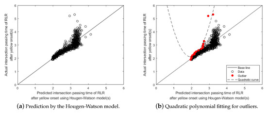
Figure 8. All-red signal extension time for RLRs: Actual vs. Prediction.

However, as one can notice, it may be too conservative sometimes to use only one prediction model to predict intersection passing times for all types of RLRs. For a certain class of RLRs, the predicted intersection passing time predicted by the model may be unnecessarily longer than needed for such RLRs. Thus, for better traffic efficiency, we develop and use different prediction models for different RLR classes to predict the intersection passing time more precisely. Figure 9 shows the prediction model of each RLR class developed by the same framework of using Hougen–Watson model and quadratic polynomial curve fitting. Having these four different prediction models corresponding to each RLR types, it is now possible to determine the necessary all-red signal extension time more effectively than using only one prediction model once the type of RLR of an incoming vehicle is correctly classified by the MC-DCNN classifier. Table 4 shows the values of the Hougen–Watson model parameters determined by the Levenberg–Marquardt algorithm for each prediction model and also the values of the coefficients for the quadratic polynomial curve fitting of outliers. Regarding the values of the quadratic polynomial curve fitting shown in the table, p₁ represents the second-order coefficient, p₂ is the first-order coefficient, and p₃ is the polynomial constant of a quadratic polynomial equation.

Figure 9. Prediction models of all red-light extension time for each RLR class type.

Table 4. Coefficients of prediction models for all-red signal extension time. (Mixed RLR represents the prediction model shown in Figure 8 and others are corresponding to models shown in Figure 9).

	Hougen–Watson Model					Polynomial Fitting
	${\mathit{\beta }}_{\mathbf{1}}$	${\mathit{\beta }}_{\mathbf{2}}$	${\mathit{\beta }}_{\mathbf{3}}$	${\mathit{\beta }}_{\mathbf{4}}$	${\mathit{\beta }}_{\mathbf{5}}$	${\mathit{p}}_{\mathbf{1}}$	${\mathit{p}}_{\mathbf{2}}$	${\mathit{p}}_{\mathbf{3}}$
Type A RLR	2.83 × 1027	−7.33 × 1026	1.15 × 1027	4.24 × 1027	5.1 × 106	4.39	−25.03	39.06
Type B RLR	0.0642	0.1003	−0.0205	0.0382	−8.89 × 105	0.57	−1.45	2.83
Type C RLR	0.1625	0.2340	−0.0210	0.1941	−2.19 × 105	−0.21	2.1	−1.32
Type D RLR	2.8061	−0.6884	0.7655	−1.3043	0.0644	0	1	0
Mixed RLR	0.0733	0.0828	−0.0133	0.0510	−7.00 × 105	2.17	−8.48	10.39

To evaluate the accuracy of the proposed multi-class intersection passing time prediction framework compared to the case of using only one prediction model, the mixed RLR model in Table 4, we use the following standard deviation of residual ${\sigma }_{est}$ defined as

$${\sigma }_{est}=\sqrt{\frac{\sum {(y-\widehat{y})}^2}{N}}$$

(3)

where N is the number of RLRs, y is the actual intersection passing time of an RLR, and $\widehat{y}$ is the predicted intersection passing time of the RLR. Table 5 is the result of the prediction accuracy of intersection passing time of RLRs measured by ${\sigma }_{est}$ for the two prediction models in the case where the prediction time after yellow onset is 3 s. As shown in the result, the proposed multi-class model has a much smaller residual standard deviation of residual compared to the case of using the mixed RLR model. This result shows that the proposed model can predict the time more accurately when an RLR will completely cross an intersection.

Table 5. Comparison of residual between mixed RLR model and proposed model.

	Mixed RLR Model	Proposed Multi-Class Model
${\sigma }_{est}$ defined in (3) for N = 1517	0.03133	0.0166

Once the intersection passing time of an RLR $\widehat{y}$ is estimated precisely, then it is relatively straightforward to determine the necessary all-red signal extension time for the RLR. A simple strategy for dynamic all-red signal extension control is as follows: If the length of the all-red signal is greater than 1 s, which is the default all-red signal length, then the length of the all-red signal is set to $\widehat{y}$ unless it is larger 5 s. In case the value of $\widehat{y}$ exceeds 5 s, then the all-red signal length is set to 5 s according to the standard.

8. Conclusions

In this paper, we proposed a system that dynamically controls all-red signal length based on the driving characteristics of Red Light Runner (RLR) vehicles to improve the overall intersection safety and efficiency. The main components of the proposed system are the Multi-Channel Deep Convolutional Neural Networks (MC-DCNN) classifier that classifies an approaching vehicle into five classes according the vehicle’s driving characteristics and the multi-level nonlinear regression model that can predict the necessary all-red signal extension time more accurately. We used the Dynamic Time Wrapping (DTW) and the Hierarchical Clustering Analysis (HCA) to carefully determine the types of clusters to be classified via MC-DCNN so that each class can be reasonably distinguishable by their driving characteristics. As a result of this multi-step classification and regression process, we validated that the proposed system can predict the actual intersection passing time of RLRs with very small prediction error and thereby it can improve both the safety as well as the efficiency of intersection traffic. In the future, we will build vehicle surveillance systems at some sections of real road intersections to collect real traffic data. Synchronized data of vehicle data and signal information will be collected, and the proposed system will be verified in a real environment. In addition, we will conduct a quantitative assessment of intersection safety and economic loss through the analysis of traffic flow due to signal extension.

References

- Betz, J.; Heilmeier, A.; Wischnewski, A.; Stahl, T.; Lienkamp, M. Autonomous Driving—A Crash Explained in Detail. Appl. Sci. 2019, 9, 5126. [Google Scholar] [CrossRef]
- Alajali, W.; Zhou, W.; Wen, S. Traffic flow prediction for road intersection safety. In Proceedings of the 2018 IEEE SmartWorld, Ubiquitous Intelligence & Computing, Advanced & Trusted Computing, Scalable Computing & Communications, Cloud & Big Data Computing, Internet of People and Smart City Innovation (SmartWorld/SCALCOM/UIC/ATC/CBDCom/IOP/SCI), Guangzhou, China, 8–12 October 2018; pp. 812–820. [Google Scholar]
- Porter, B.E.; Berry, T.D.; Harlow, J.; Vandecar, T. A Nationwide Survey of Red Light Running: Measuring Driver Behaviors for the ‘Stop Red Light Running Program’. 1999. Available online: http://citeseerx.ist.psu.edu/viewdoc/download?doi=10.1.1.468.6543&rep=rep1&type=pdf (accessed on 31 July 2020).
- McGee, H., Sr.; Moriarty, K.; Gates, T.J. Guidelines for timing yellow and red intervals at signalized intersections. Transp. Res. Rec. 2012, 2298, 1–8. [Google Scholar] [CrossRef]
- Retting, R.A.; Greene, M.A. Influence of traffic signal timing on red-light running and potential vehicle conflicts at urban intersections. Transp. Res. Rec. 1997, 1595, 1–7. [Google Scholar] [CrossRef]
- Zheng, Y.; Liu, Q.; Chen, E.; Ge, Y.; Zhao, J.L. Exploiting multi-channels deep convolutional neural networks for multivariate time series classification. Front. Comput. Sci. 2016, 10, 96–112. [Google Scholar] [CrossRef]
- Ferraris, G.B.; Donati, G. A powerful method for Hougen—Watson model parameter estimation with integral conversion data. Chem. Eng. Sci. 1974, 29, 1504–1509. [Google Scholar] [CrossRef]
- Ren, Y.; Wang, Y.; Wu, X.; Yu, G.; Ding, C. Influential factors of red-light running at signalized intersection and prediction using a rare events logistic regression model. Accid. Anal. Prev. 2016, 95, 266–273. [Google Scholar] [CrossRef]
- Li, M.; Chen, X.; Lin, X.; Xu, D.; Wang, Y. Connected vehicle-based red-light running prediction for adaptive signalized intersections. J. Intell. Transp. Syst. 2018, 22, 229–243. [Google Scholar] [CrossRef]
- Chen, X.; Zhou, L.; Li, L. Bayesian network for red-light-running prediction at signalized intersections. J. Intell. Transp. Syst. 2019, 23, 120–132. [Google Scholar] [CrossRef]
- de Goma, J.C.; Bautista, R.J.; Eviota, M.A.J.; Lopena, V.P. Detecting Red-Light Runners (RLR) and Speeding Violation through Video Capture. In Proceedings of the 2020 IEEE 7th International Conference on Industrial Engineering and Applications (ICIEA), Bangkok, Thailand, 16–21 April 2020; pp. 774–778. [Google Scholar]
- Jahangiri, A.; Rakha, H.; Dingus, T.A. Red-light running violation prediction using observational and simulator data. Accid. Anal. Prev. 2016, 96, 316–328. [Google Scholar] [CrossRef]
- Elias, S.; Ghafurian, M.; Samuel, S. Effectiveness of Red-Light Running Countermeasures: A Systematic Review. In Proceedings of the 11th International Conference on Automotive User Interfaces and Interactive Vehicular Applications, Utrecht, The Netherlands, 21–25 September 2019; pp. 91–100. [Google Scholar]
- Quiroga, C.; Kraus, E.; van Schalkwyk, I.; Bonneson, J. Red Light Running: A Policy Review. 2003. Available online: https://citeseerx.ist.psu.edu/viewdoc/download?doi=10.1.1.198.4032&rep=rep1&type=pdf (accessed on 31 July 2020).
- Retting, R.A.; Ferguson, S.A.; Farmer, C.M. Reducing red light running through longer yellow signal timing and red light camera enforcement: Results of a field investigation. Accid. Anal. Prev. 2008, 40, 327–333. [Google Scholar] [CrossRef]
- Collotta, M.; Pau, G.; Scatà, G.; Campisi, T. A dynamic traffic light management system based on wireless sensor networks for the reduction of the red-light running phenomenon. Transp. Telecommun. J. 2014, 15, 1–11. [Google Scholar] [CrossRef]
- Cascetta, E.; Gallo, M.; Montella, B. Optimal signal setting on traffic networks with stochastic equilibrium assignment. In Proceedings of the TRISTAN III-Triennial Symposium on Transportation Analysis, San Juan, Puerto Rico, 17–23 June 1998; Volume 2. [Google Scholar]
- Adacher, L.; Cipriani, E. A surrogate approach for the global optimization of signal settings and traffic assignment problem. In Proceedings of the 13th International IEEE Conference on Intelligent Transportation Systems, Funchal, Portugal, 19 September 2010; pp. 60–65. [Google Scholar]
- D’Acierno, L.; Gallo, M.; Montella, B. An ant colony optimisation algorithm for solving the asymmetric traffic assignment problem. Eur. J. Oper. Res. 2012, 217, 459–469. [Google Scholar] [CrossRef]
- Sbayti, H.; Lu, C.C.; Mahmassani, H.S. Efficient implementation of method of successive averages in simulation-based dynamic traffic assignment models for large-scale network applications. Transp. Res. Rec. 2007, 2029, 22–30. [Google Scholar] [CrossRef]
- Kashani, A.T.; Amirifar, S.; Bondarabadi, M.A. Analysis of Driver and Vehicle Characteristics Involved in Red-Light Running Crashes: Isfahan, Iran. Iran. J. Sci. Technol. Trans. Civ. Eng. 2020, 1–7. [Google Scholar] [CrossRef]
- Fu, C.; Xiong, Y.; Zhang, Y.; Zhang, W.; Liu, Y. A novel model of increasing block fine for red-light running recidivism. Adv. Mech. Eng. 2019, 11, 1687814019828047. [Google Scholar] [CrossRef]
- Zhang, L.; Zhou, K.; Zhang, W.B.; Misener, J.A. Prediction of red light running based on statistics of discrete point sensors. Transp. Res. Rec. 2009, 2128, 132–142. [Google Scholar] [CrossRef]
- Zhu, X.; Yuan, Y.; Hu, X.; Chiu, Y.C.; Ma, Y.L. A Bayesian Network model for contextual versus non-contextual driving behavior assessment. Transp. Res. Part C Emerg. Technol. 2017, 81, 172–187. [Google Scholar] [CrossRef]
- Karl, I.; Berg, G.; Ruger, F.; Farber, B. Driving behavior and simulator sickness while driving the vehicle in the loop: Validation of longitudinal driving behavior. IEEE Intell. Transp. Syst. Mag. 2013, 5, 42–57. [Google Scholar] [CrossRef]
- Senin, P. Dynamic Time Warping Algorithm Review; Information and Computer Science Department University of Hawaii at Manoa: Honolulu, HI, USA, 2008. [Google Scholar]
- Khan, L.; Awad, M.; Thuraisingham, B. A new intrusion detection system using support vector machines and hierarchical clustering. VLDB J. 2007, 16, 507–521. [Google Scholar] [CrossRef]
- Chang, C.C.; Lin, C.J. LIBSVM: A library for support vector machines. ACM Trans. Intell. Syst. Technol. (TIST) 2011, 2, 1–27. [Google Scholar] [CrossRef]
- Huang, K.S.; Chiu, P.J.; Tsai, H.M.; Kuo, C.C.; Lee, H.Y.; Wang, Y.C.F. Redeye: Preventing collisions caused by red-light running scooters with smartphones. IEEE Trans. Intell. Transp. Syst. 2015, 17, 1243–1257. [Google Scholar] [CrossRef]
- Franc, V.; Hlavác, V. Multi-class support vector machine. In Proceedings of the Object Recognition Supported by User Interaction for Service Robots, Quebec City, QC, Canada, 11–15 August 2002; Volume 2, pp. 236–239. [Google Scholar]
- Debnath, R.; Takahide, N.; Takahashi, H. A decision based one-against-one method for multi-class support vector machine. Pattern Anal. Appl. 2004, 7, 164–175. [Google Scholar] [CrossRef]
- Setiowati, S.; Zulfanahri; Franita, E.L.; Ardiyanto, I. A review of optimization method in face recognition: Comparison deep learning and non-deep learning methods. In Proceedings of the 2017 9th International Conference on Information Technology and Electrical Engineering (ICITEE), Phuket, Thailand, 12–13 October 2017; pp. 1–6. [Google Scholar]
- Wang, C.; Han, Y.; Wang, W. An end-to-end deep learning image compression framework based on semantic analysis. Appl. Sci. 2019, 9, 3580. [Google Scholar] [CrossRef]
- Fawaz, H.I.; Forestier, G.; Weber, J.; Idoumghar, L.; Muller, P.A. Deep learning for time series classification: A review. Data Min. Knowl. Discov. 2019, 33, 917–963. [Google Scholar] [CrossRef]
- Sainath, T.N.; Weiss, R.J.; Wilson, K.W.; Li, B.; Narayanan, A.; Variani, E.; Bacchiani, M.; Shafran, I.; Senior, A.; Chin, K.; et al. Multichannel signal processing with deep neural networks for automatic speech recognition. IEEE/ACM Trans. Audio Speech Lang. Process. 2017, 25, 965–979. [Google Scholar] [CrossRef]
- Nugraha, A.A.; Liutkus, A.; Vincent, E. Multichannel audio source separation with deep neural networks. IEEE/ACM Trans. Audio Speech Lang. Process. 2016, 24, 1652–1664. [Google Scholar] [CrossRef]
- Dennis, J.E., Jr.; Gay, D.M.; Walsh, R.E. An adaptive nonlinear least-squares algorithm. ACM Trans. Math. Softw. (TOMS) 1981, 7, 348–368. [Google Scholar] [CrossRef]
- Newville, M.; Stensitzki, T.; Allen, D.B.; Rawlik, M.; Ingargiola, A.; Nelson, A. LMFIT: Non-Linear Least-Square Minimization and Curve-Fitting for Python; Astrophysics Source Code Library (ASCL): Houghton, MI, USA, 2016. [Google Scholar]
- Radhakrishnan, P.; Mathew, T.V. Passenger car units and saturation flow models for highly heterogeneous traffic at urban signalised intersections. Transportmetrica 2011, 7, 141–162. [Google Scholar] [CrossRef]
- Koonce, P.; Rodegerdts, L. Traffic Signal Timing Manual; Technical Report; Federal Highway Administration: Washington, DC, USA, 2008. [Google Scholar]
© 2020 by the authors. Licensee MDPI, Basel, Switzerland. This article is an open access article distributed under the terms and conditions of the Creative Commons Attribution (CC BY) license (http://creativecommons.org/licenses/by/4.0/).