A Low-Cost, Small-Size, and Bluetooth-Connected Module to Detect Faults in Rolling Bearings

Abstract

Condition monitoring techniques have been successfully applied to detect damaged bearings. However, the signal acquisition and the subsequent processing are typically outsourced to expensive data acquisition boards and complex software, resulting in expensive solutions. As a side effect, the integration of condition monitoring systems in wireless sensor networks can be tough to achieve. Aiming to overcome such issues, a low-cost and small-size electronic module to be placed in the proximity of the bearing to be monitored was developed. The acoustic signal delivered by the bearing is acquired, and the corresponding frequency spectrum is evaluated on-board. Based on that, the developed module automatically detects the presence of defects and notifies the remote controller via a wireless connection only when a fault is detected, thus avoiding the use of data cables whilst minimizing the amount of transferred data. Experimental tests carried out on the proposed system assessed the accuracy of the evaluated frequency spectrum, resulting in an amplitude error within $\pm 0.6\%$, as well as the fault detection capability in the presence of environmental acoustic noise.

1. Introduction

The reliability of mechanical systems has become an increasingly major topic, as malfunctions are responsible for extra costs, non-operating time, and unscheduled maintenance. As far as rotating machines are concerned, it is well established that rolling bearings are one of the root causes of such failures, indeed, almost 50% of the faults occurring to electric motors is ball- or roller bearing-related [1]. As a consequence, the monitoring of such components is necessary to avoid unwanted malfunctions, leading researchers and practitioners to investigate condition monitoring techniques even more performing and accurate. When dealing with condition monitoring, a signal that contains data on the dynamic response of the structure to be monitored is acquired, and some processing technique is applied to such signals in order to detect the presence of faults, and possibly to identify them and to estimate their size. As far as the monitoring of rolling bearing is concerned, usually the acquired signal corresponds to the vibrations sensed in the proximity to the bearing by means of a transducer, i.e., an accelerometer, whereas the processing techniques that can be found in the literature are the most varied. A comprehensive review of such processing methods can be found in [2,3,4]. More recently, approaches based on machine learning, as those shown in [5], were applied to a vibration dataset in order to identify faulty bearings. Further investigations on such topics regard the enhancement of the fault detection in the presence of noise, as in [6,7,8].

Besides the exploitation of vibrations, acoustic emission (AE) has emerged as a valid solution, in particular regarding early-stage damages where the spall has not yet been formed on the surface [9] of the inner or outer ring. The cyclostationary of such a kind of signal can be even exploited to enhance the detection of bearing faults, as reported in [10]. However, the main drawback of AE is the required sampling frequency, which is typically higher than 1 MHz [11], resulting in a huge amount of sampled data and expensive acquisition hardware. In between the AE and the vibrations, the acoustic noise, i.e., up to 20 kHz, can be exploited to detect the presence of defects, as reported in [12,13], where conventional and low-cost microphones were exploited achieving interesting results. The major benefit in the use of microphones is that no contact with the cage is required, meaning that the transducer can be placed in the most convenient location as close as possible to the bearing to be monitored.

Regardless of the kind of acquired signal, it is worth noticing that the acquisition is outsourced to high-performance data acquisition board (DAQ), as in [14], and that the subsequent signal processing is performed by means of high-level software, e.g., Matlab, resulting in an expensive and complex to be integrated monitoring system. Some previous works have dealt with such issues using a Digital Signal Processor (DSP) [15] or a Field Programmable Gate Array (FPGA) [16], however they are still rather expensive solutions.

Such aspects may prevent the bearing monitoring system from being successfully integrated in low-cost and wireless nodes, which can be the building blocks of more complex Wireless Sensor Networks (WSN). The design of wireless nodes for the bearing monitoring was already investigated in previous works. More precisely, the authors of [17] proposed a wireless module that collects the signal from an accelerometer and sends it to a server using a proprietary protocol. Similarly, in [18], data from different sensors are acquired, filtered and sent to a central unit to determine the causes of faults in induction motors. In [19], a machine learning approach is exploited to analyze the dataset collected by the nodes, and the number of nodes to maximize their life-time is investigated performing simulations. It is worth noticing that the amount of data to be transferred is an important aspect to be considered in a wireless link, as it affects the power consumption, the required bandwidth, and also the reliability of the communication, eventually. In order to address such issue, compression techniques, such as those shown in [20,21], were proposed to minimize the amount of raw data to be transferred, without affecting the fault detection. Besides such solutions, a different approach consists in the distributed computing paradigm, where each node is provided with sufficient computational capability to execute some part or the entire signal processing. The authors of [22] proposed a system where the frequency spectrum of the envelope is evaluated by the module itself, and then wirelessly transferred to a host computer, which is also responsible for the evaluation of the optimum band-pass filter to be applied.

Nonetheless, none of the aforementioned works proposed a low-cost wireless module able to detect the faults locally. In such a way, the data transfer can be truly minimized, as the node would occupy the wireless link only in the presence of a fault. Aiming to minimize the cost of such a module, a low-cost microphone and a microcontroller with an integrated radio transceiver are exploited. In such a way, the acoustic emission delivered by the bearing is acquired and processed, and the faults are detected, with all the steps locally performed. This work proposes such a wireless module, where the cost and hardware and software complexity are kept at minimum. Indeed, the standard Bluetooth Low Energy wireless link allows for a on-the-fly configuration of the module from several compatible devices, thus achieving both user and machine-to-machine (M2M) interaction. By choosing target designs of low cost and small size, it results in different benefits, as the former allows one to place more modules, and the latter to position the proposed system in the most convenient location closed to the bearing to be monitored. In such a way, even in the presence of a noisy environment, the module is able to assess the healthy status of the bearing to be monitored.

The paper is organized as follows. In Section 2, the processing technique and its optimization are discussed. In Section 3, the proposed system is introduced and its main functional blocks are analyzed, along with the fault detection algorithm. Experimental results, regarding the computational performance and the detection capability of the designed module in the presence of environmental noise, are discussed in Section 4, and final conclusions are drawn in Section 5.

2. Evaluation of the Frequency Spectrum

2.1. Fundamental Frequencies of Rolling Bearings

Rolling bearing faults are typically due to misalignment, lack of lubrication, or excessive load. A crack may origin at subsurface or at surface level, and gradually increases up to become a spall, i.e., a groove removal from the surface of the inner or the outer race. In such a case, the rolling bearing is definitely damaged and it has to be substituted. When the defect is localized to the inner or outer ring, the rolling elements, i.e., the rollers or the balls, impact on it at a given frequency, which depends on the bearing geometry and on the rotation frequency. The ball pass frequency of the outer race ($BPFO$) and the ball-pass frequency of the inner race ($BPFI$) and can be evaluated as [23]

$$BPFO=\frac{Z{f}_r}{2}\left(1-\frac{d}{D}cos\alpha \right)$$

(1)

$$BPFI=\frac{Z{f}_r}{2}\left(1+\frac{d}{D}cos\alpha \right),$$

(2)

where Z is the number of rolling elements, $f_r$ is the inner rotation frequency, d is the rolling element diameter, D is the pitch diameter, and $\alpha$ is the contact angle. Similarly, if the defect is located on the cage or on a rolling-element, it will occur every Fundamental Train Frequency ($FTF$) or Ball Spin Frequency ($BSF$), respectively. Similarly, such frequencies can be evaluated as

$$FTF=\frac{f_r}{2}\left(1-\frac{d}{D}cos\alpha \right),$$

(3)

$$BSF=\frac{D}{2d}\left(1-{\left(\frac{d}{D}cos\alpha \right)}^2\right).$$

(4)

The impact of a ball or a roller on a defect generates an impulsive transient, which will be reflected on both the vibrations and on the acoustic signal delivered by the bearing. Such an impulsive event excites the resonant frequencies of the structure, and, if the operating conditions are unchanged, it is cyclically repeated every $BPFI$, $BPFO$, $FTF$, or $BSF$, depending on the location of the defect. Thus, the more convenient way to check whether a defect is present or not, is to verify the amplitude of the frequency spectrum of the acquired signal at the defect fundamental frequencies. It can be noticed that such defect fundamental frequencies are valid both for ball and roller bearings [24]. Indeed, when a defect arises, the amplitude of the spectrum at the corresponding frequency will increase. On the other hand, it is possible to band-pass filter the signal, evaluate its envelope signal and the corresponding frequency spectrum, and finally to check the amplitudes at the same fundamental frequencies. Indeed, the frequency spectrum evaluation is the most expensive computational step, thus it should be carefully optimize referring to the target application. As such data processing must be performed by the module itself, and that dedicated accelerating hardware, such as FPGA or Application Specific Integrated Circuit (ASIC), cannot be exploited to keep the cost of the developed module low, a microcontroller should be used. A discussion on how to reduce the computational effort of the evaluation of the frequency spectrum is presented in the remainder of this section.

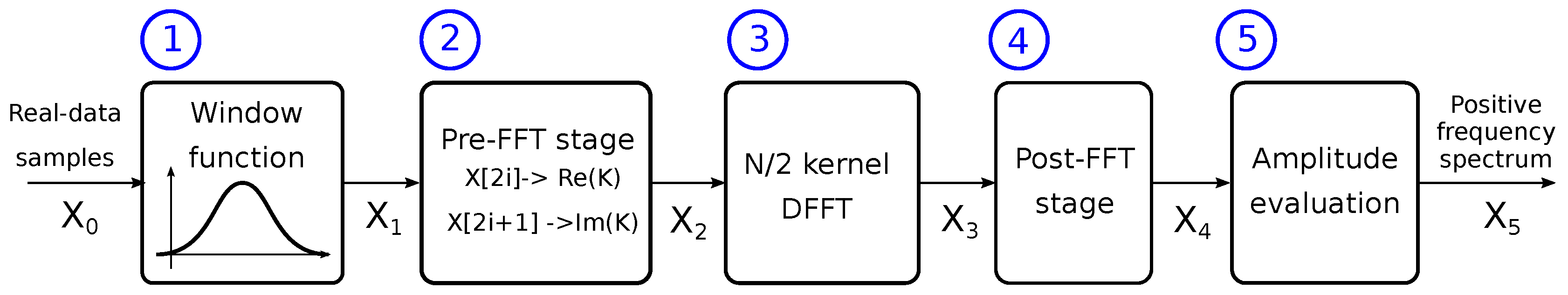
2.2. Optimized Discrete Fast Fourier Transform

As far as the detection of faulty bearing is concerned, the amplitudes of the frequency spectrum should be evaluated to verify their values at the defect fundamental frequencies, eventually. In order for the signal processing to be performed on-board, an efficient and accurate algorithm is required. The most famous and popular one is the Discrete Fast Fourier Transform (DFFT) algorithm [25], where the $N_s$ elements of the input sequence $X\left[n\right]$ are multiplied by constants, the so-called twiddle factors, and summed together in the consecutive stages of the algorithm. If the length of the input sequence $N_s$ is a power of 2, then the resulting complexity is $O\left(N_{s}log\left(N_s\right)\right)$. The required operations are sums and multiplications, which are highly optimized for both integers and floating data in modern microcontroller architectures, and the computation of the twiddle factors, where sine and cosine functions are required. Such twiddle factors can be evaluated only once and then stored in a buffer, as their values only depends on $N_s$. Even though more performing algorithm exists in terms of required operations, e.g., the Fast Hartley Transform (FHT), the radix-2 DFFT was exploited in what follows since it requires the lowest data memory [26], which is an important aspect in a limited-resources design. As far as the detection of bearing faults is concerned, the input sequence ($X\left[n\right]$) is the readout of analog sensors, thus its imaginary part is always zero. As a consequence, symmetry properties can be exploited to reduce the amount of required operations, resulting an optimized DFFT for real data [27].

As the fault assessment is based on the amplitudes of the spectrum at given frequencies, the evaluation of such frequency spectrum must be reliable. However, the spectral leakage phenomenon, which occurs when the sampling frequency, is not an integer number of the populated frequencies, may result in an underestimation, up to 3 dB, of some spectral components [28]. In a such a case, a faulty bearing may be detected as a healthy one, resulting in a false negative. To address this issue, the input sequence ($X\left[n\right]$) can be multiplied by a proper windowing function, so that $X\left[n\right]$ smoothly reaches zero at its boundaries and the spectral leakage phenomenon is strongly reduced. Different windows, e.g., top flat, Hann-2, Hann-4, or Blackman, may serve this scope.

Aiming to perform such computations on board, the required steps are reported in Figure 1, where the encircled numbers refer to the step number and where the data array at the input of the i-th step is named $X_{i-1}$. A detail description of each step is reported in what follows.

• Step 1 The windowing function, which was previously evaluated for the $N_s$ samples and stored in the $K_{window}\left[n\right]$ array, is multiplied by the input sequence $X_0\left[n\right]$ of the sampled data, resulting in the $X_1\left[n\right]$ output array.

  $$X_1\left[n\right]=X_0\left[n\right]·K_{window}\left[n\right]$$

  (5)
• Step 2 The even components of $X_1\left[n\right]$ are placed in the real part of $X_2\left[n\right]$, and the odd ones in the imaginary part, so that $X_2\left[m\right]$ is a complex data array of length $N_s/2$.

  $$\mathsf{Re}\left(X_2\left[m\right]\right)=X_1\left[2n\right],\mathsf{Im}\left(X_2\left[m\right]\right)=X_1[2n+1],n=0,\dots ,N_s/2$$

  (6)
• Step 3 The standard Cooley–Tukey radix-2 transform [25] is evaluated on the basis of the $X_2\left[m\right]$ array, resulting in $X_3\left[m\right]$. It is worth noticing that the length of the input sequence is $N_s/2$, which is one only half of the original input sequence ($X_0\left[n\right]$).
• Step 4 Real and imaginary parts have to be recombined together to reconstruct the $N_s/2+1$ samples of the positive frequency spectrum as

  $$\begin{array}{c}\hfill Re\left(X_4\left[k\right]\right)=A_r\left[k\right]Re\left(X_3\right)\left[k\right]-A_i\left[k\right]Im\left(X_3\right)\left[k\right]+B_r\left[k\right]Re\left(X_3\right)[N-k]+B_i\left[k\right]Im\left(X_3\right)[N-k]\end{array}$$

  (7)

  $$\begin{array}{c}\hfill Im\left(X_4\left[k\right]\right)=A_r\left[k\right]Im\left(X_3\right)\left[k\right]+A_i\left[k\right]Re\left(X_3\right)\left[k\right]+B_i\left[k\right]Re\left(X_3\right)[N-k]-B_r\left[k\right]Im\left(X_3\right)[N-k]\end{array}$$

  (8)

  where $A_r,B_r$ and $A_i,B_i$ are the real part and the imaginary part of the $A,B$ coefficients evaluated from the twiddle factors ($W_{N_s}^k$), respectively, as

  $$A\left[k\right]=\frac{1}{2}\left(1-j{W}_{N_s}^k\right)B\left[k\right]=\frac{1}{2}\left(1+j{W}_{N_s}^k\right)$$

  (9)
• Step 5 The amplitude of the frequency spectrum can be evaluated, eventually. Such an array has to be multiply by the inverse of the coherent gain of the exploited windowing function.

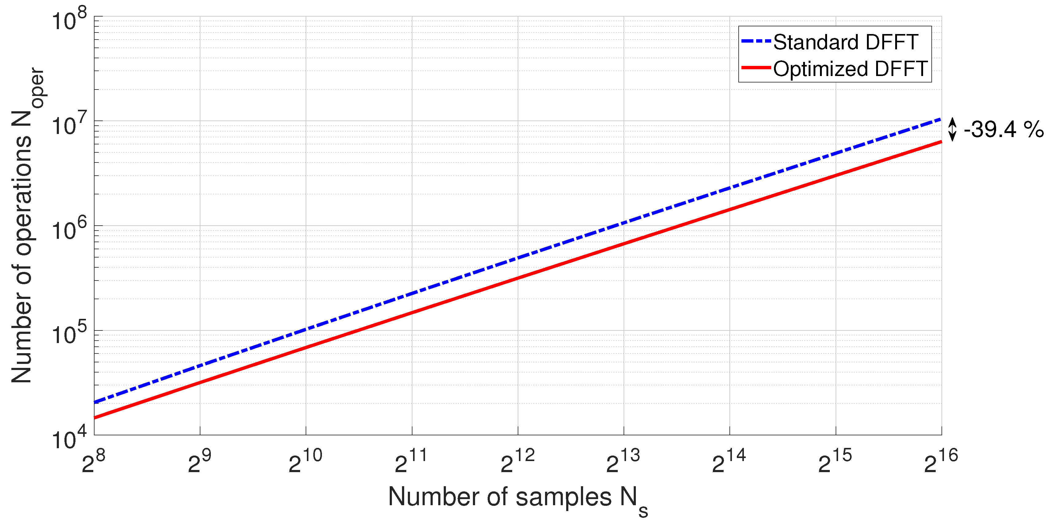
2.3. Comparison with Standard Algorithm

To assess the performance of the optimized algorithm with respect to the traditional one, i.e., the one non-optimized for real data, the number of multiplications and sums ($N_{\mathrm{oper}}$) was considered as a figure of merit. Indeed, the number of operations affects both the computation time and the power consumption, thus it should be minimized, definitely. As in modern microcontroller architecture, e.g., Advanced RISC Machine (ARM), the sum and the multiplication required a single operation to be performed, provided that the data is in fixed-point notation [29], it makes sense to consider their sum. Figure 2 shows the number of operation for different $N_s$, in case of the traditional DFFT algorithm (dashed-dot line) and the optimized one for real data (continuous line). Even though step 4 introduces an overhead with respect to the evaluation of a $N_s/2$ DFFT, the latter outperforms the former whatever $N_s$ is, with a percentage reduction varying from 29% ($N_s=2^8$) up to 39.4% in the best case, i.e., $N_s=2^{16}$.

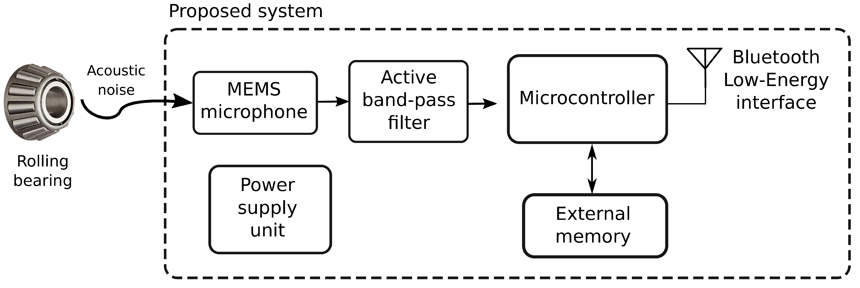
3. Proposed Solution

In order for the proposed system to detect a faulty bearing and wirelessly notify a remote controller, different hardware and software blocks have to be combined together. As the acoustic noise is exploited, a microphone is required as a transducer, so that its output signal can be sampled and processed by the microcontroller itself. Then, the optimized DFFT has to be executed to evaluate the frequency spectrum of the acquired signal, and the subsequent fault detection algorithm determines whether the rolling bearing is damaged or not. If one or more defects are present, the microcontroller notifies the remote controller by means of the wireless link, which is based on the Bluetooth Low-Energy standard protocol. Moreover, the wireless connection allows the remote controller to access and modify the configuration of the module on-the-fly, resulting in a highly reconfigurable solution. A schematic view of the proposed module is shown in Figure 3, and an in-depth description of each block will be provided in the remainder of this Section.

3.1. Signal Conditioning and Data Acquisition

A Microelectromechanical System (MEMS) microphone was exploited as a transducer because of its low cost, small size, and bandwidth. Before being sampled, the analog signal is band-pass filtered. Such an operation is performed by means of an audio amplifier, in order to filter the high frequency components that would cause aliasing and to adapt the signal to the Analog-to-Digital Converter (ADC) input range. The frequency band is [37 Hz, 20 kHz] and the in band gain is approximately 200. Subsequently, a 12 bit ADC, which is inside the microcontroller and provided with an internal voltage reference, digitizes the filtered input signal at a sampling frequency $f_s$.

3.2. Frequency Spectrum Evaluation

The computation of the frequency spectrum of the sampled signal is performed accordingly to the algorithm discussed in the previous section. More precisely, the data may be represented either in fixed-point (16 bit) or in floating-point (32 bit) notation, but the former allows one to halve the required memory. Due to the limited size of the memory available on the microcontroller, an external Static Random Access Memory (SRAM) was added in case the configuration of the system requires $N_s>2^{12}$.

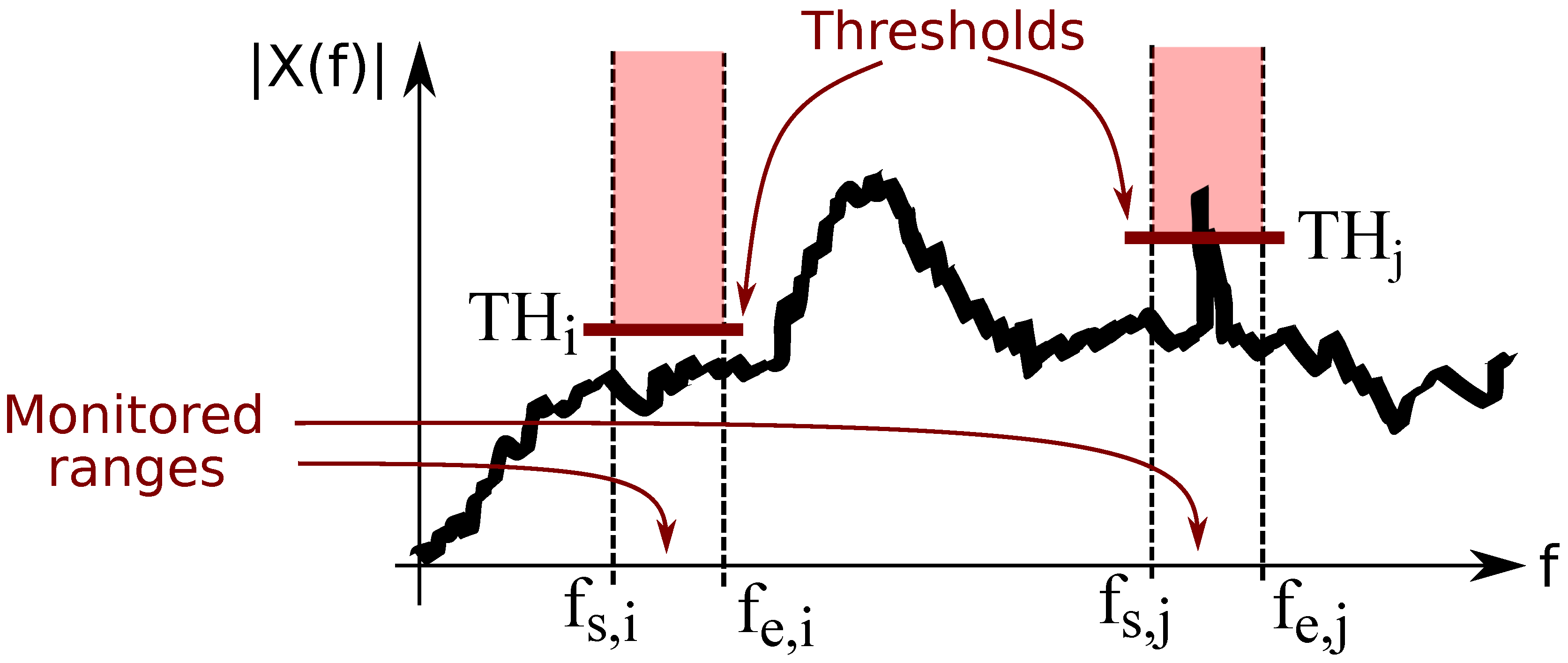
3.3. Detection Algorithm

The amplitude of the frequency spectrum $\left|X\right(f\left)\right|$, which was evaluated in the previous step, has to be compared against a set of given thresholds for the frequency ranges to be monitored. More precisely, each range $i=0,\dots ,M-1$ is characterized by the frequency interval $[f_{s,1},f_{e,i}]$ and by a threshold $T{H}_i$, as shown in Figure 4. The detection algorithm works as follows; for each range $i=0,\dots ,M-1$, if $\forall f\in [f_{s,1},f_{e,i}],\left|X\left(f\right)\right|<T{H}_i$, then no defect occurs; otherwise, such range is pointed one. The monitored ranges are centered around a specific defect fundamental frequency ($BPFO$, $BPFI$, etc.), and provide a sufficiently large frequency interval to account for uncertainties. As the frequency ranges are affected by the geometry of the bearing and on its operating condition, whereas the thresholds are related to the noise floor, which is strictly related to the particular environment, they can be entirely configured using the wireless link, thus giving the maximum flexibility to the designed system.

3.4. Bluetooth Low-Energy Interface

As far as the wireless link is concerned, a standard protocol in the 2.4 GHz Industrial, Scientific, and Medical (ISM) band was preferred rather than a proprietary one, which would be more thought to integrate with other devices and systems. Among the other standard protocols operating in the same frequency band, the Bluetooth Low-Energy (BLE) was chosen because of its elevated spread, which results in low-cost radio transceivers, several compatible devices, and its good radio performance (10 m range). The fundamental entity that can be transferred between two BLE devices is the called characteristic, and it is at least 16 byte longer [30]. As the read (the write) of a single characteristic requires a significant overhead from the reader (writer) point of view, the number of characteristics should definitely be minimized. Taking into account such two aspects, a set of four characteristics, i.e., configuration, command, ranges set-up, and over-threshold peaks, was adopted. The configuration characteristic allows one to control $f_s$, $N_s$, and the windowing function, the command one to set the module in idle state, to force a signal acquisition and the postprocessing, or to perform the fault detection cyclically. The parameters of the ranges to be monitored, as well as their number, can be modify through the ranges characteristic, and finally the amplitudes of the frequency spectrum that exceed the given thresholds, and the corresponding frequencies, are pointed out in the over-threshold peaks characteristic. The list of parameters accessible through the BLE interface are listed in

Table 1. Configurable parameters via Bluetooth Low-Energy.

Parameter	Value
Sampling frequency ($f_s$)	100 Hz to 50 kHz
Number of samples ($N_s$)	256–65832
Windowing function	No window, Hann-2, Hann-4, top flat, Blackman
How often acquire and process signal	30 s to 100 min
Parameters of i-th range	$T{H}_i,f_{s,1},f_{e,i}$

, and the size of transferred data in

Table 2. Size of characteristics transferred via Bluetooth Low-Energy.

Characteristic	Size
Configuration	12 bytes
Command	3 bytes
Range setup	6 bytes for range, maximum 21 ranges
Over-threshold peaks	6 bytes for peak, maximum 21 peaks

. Moreover, the exploitation of the notification feature allows the proposed module to notify the remote controller only when the over-threshold peaks characteristic changes, meaning that the remote controller is not required to continuously read such characteristic.

4. Results and Discussion

Aiming to assess what presented so far, a prototype of the proposed module was realized and experimental tests were carried out to verify the performance of the optimized DFFT algorithm and the fault detection capability in the presence of environmental noise. The corresponding results are discussed in the remainder of the paper.

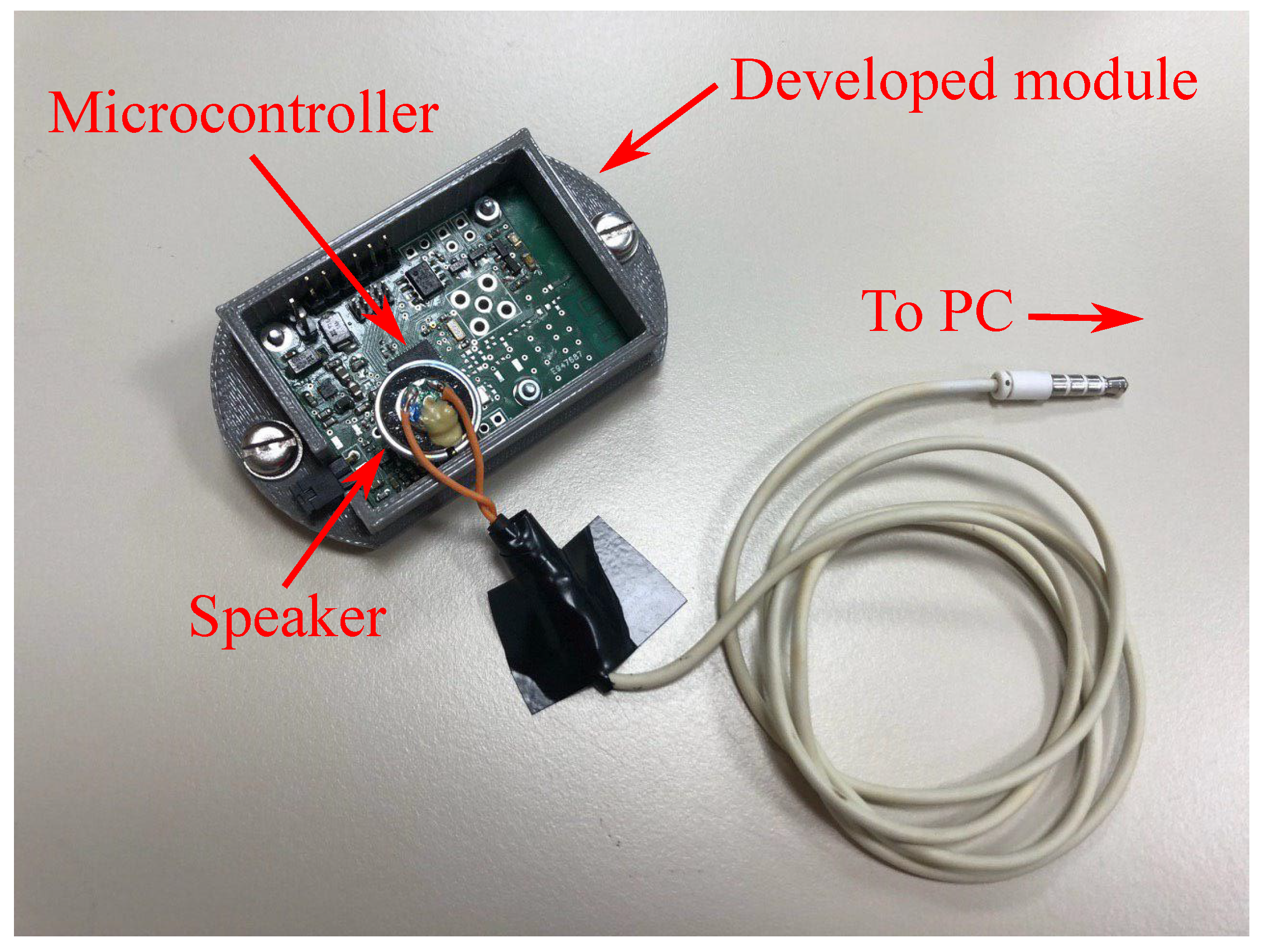
4.1. Proposed Prototype

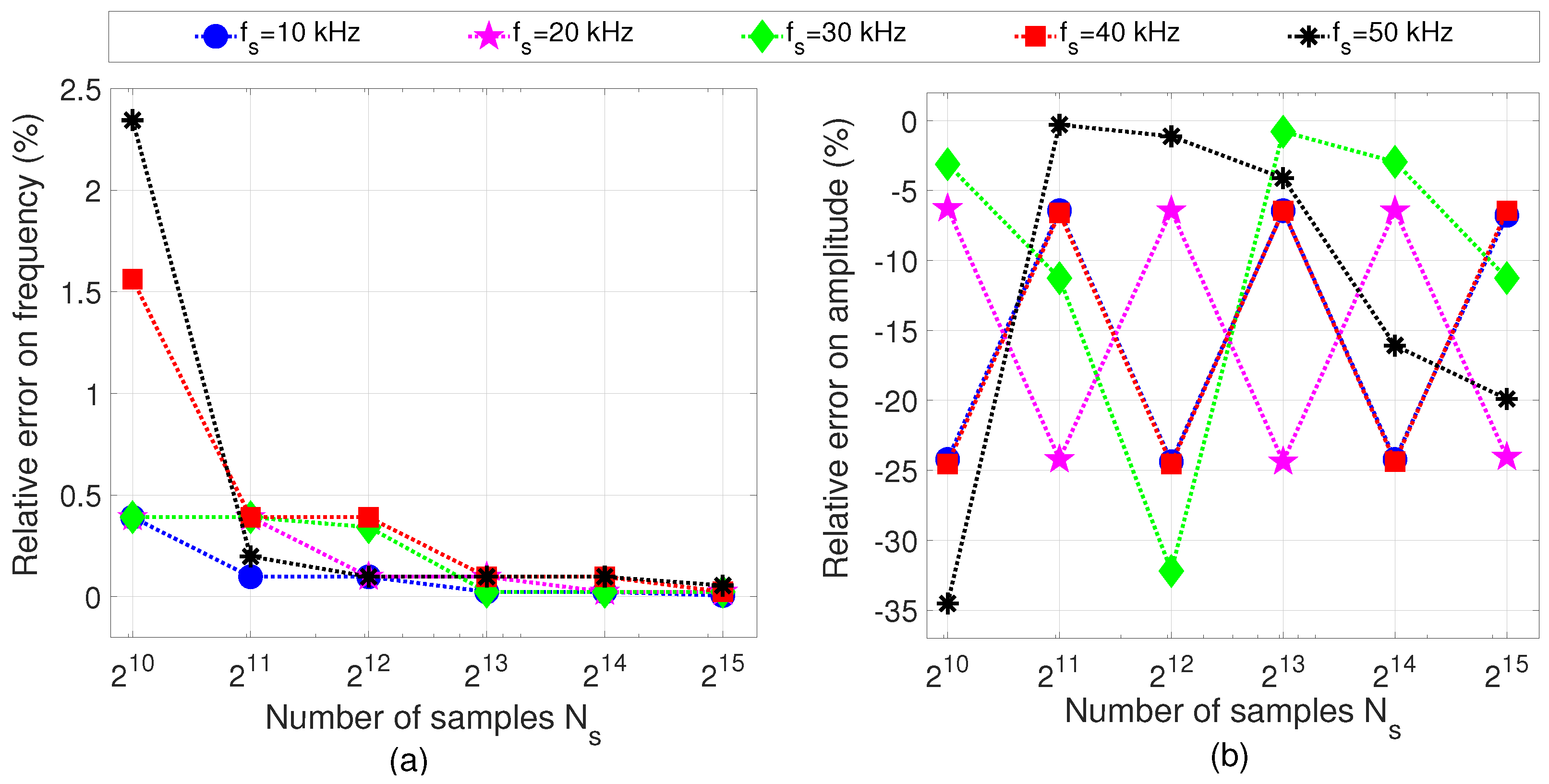
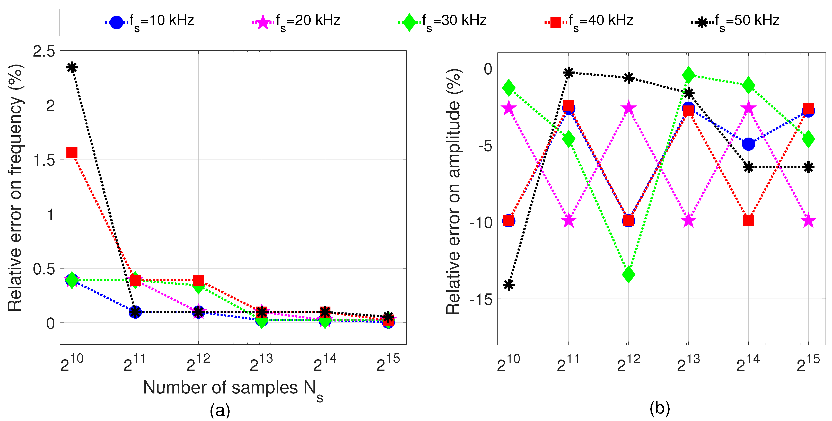
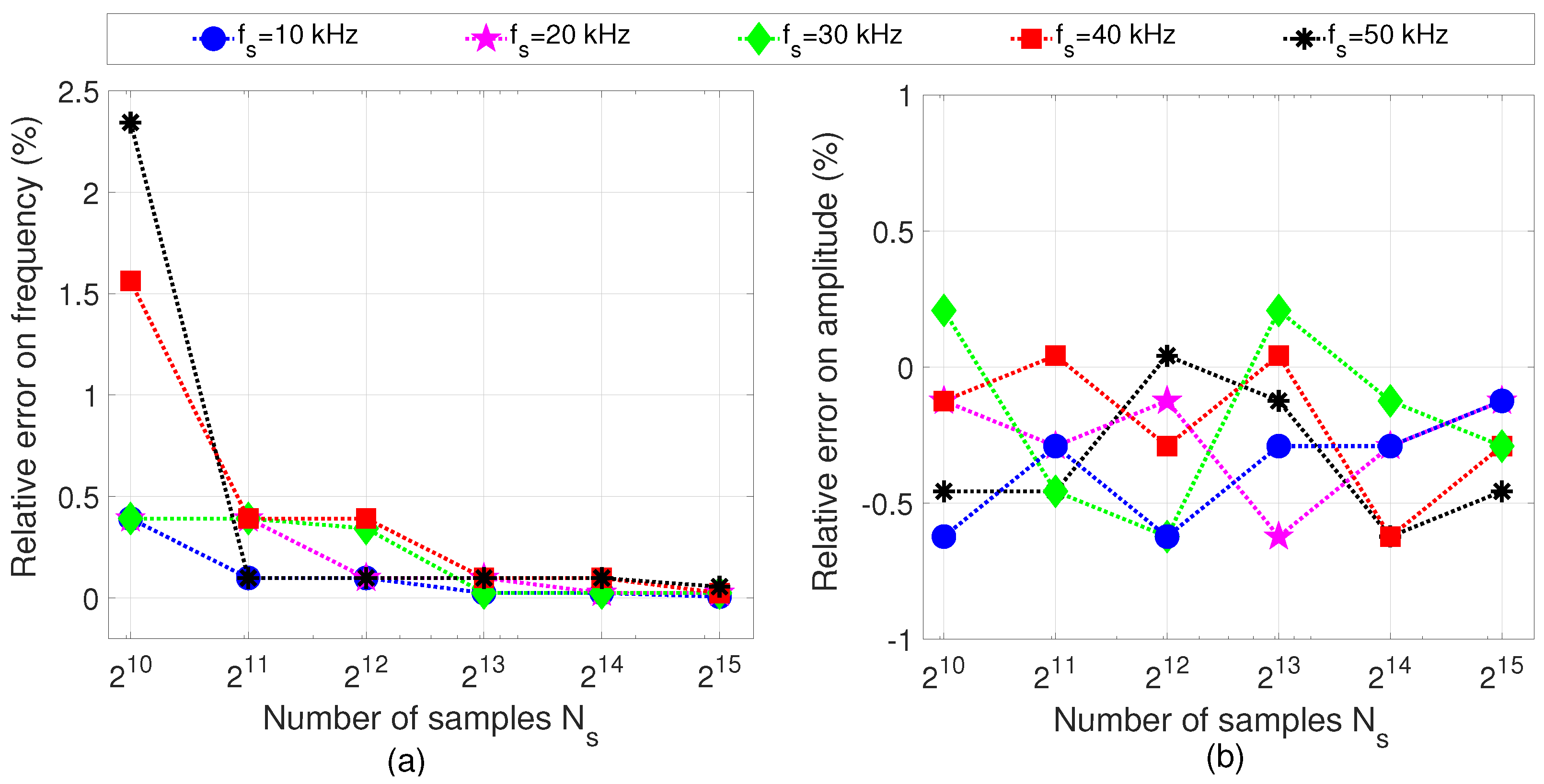
A Printed Circuit Board (PCB) was designed and realized to include all the required components for the module to work as a stand-alone system. The module is provided with a power supply unit, which regulates the DC input supply voltage, ranging in [8 V, 16 V], to a lower value (3.3 V) to power all the components. No data cables are required since both configuration and data transfer are outsourced to the wireless link. A microcontroller, with a on-board BLE transceiver, was exploited to minimize the number of components. The overall dimensions of the module, i.e., 47.25 mm × 32.35 mm, allow it for being located in a confined space.

4.2. FFT Accuracy

As the algorithm for the fault detection is based on the exceeding of given thresholds in a set of frequency ranges, the accuracy of the acquisition channel and of the spectrum evaluation plays a key role in the capability of the system to detect faults when they occur, avoiding false positives and false negatives. In order to characterized the acquisition channel and the DFFT algorithm in terms of frequency offset and amplitude error, a sinusoidal signal was applied to the ADC input, it was sampled, and the frequency spectrum evaluated by the microcontroller. The sinusoidal input signal is characterized by 1 kHz fundamental frequency ($f_{0,nom}$), 600 mV average value, and 700 mV peak amplitude ($A_{0,nom}$). In such a way, the input range of the ADC is almost entirely covered, and the quantization error is minimized. The nominal parameters of such a signal were measured using a 6-digit multimeter and a counter, and compared against the ones extracted from the frequency spectrum evaluated by the microcontroller, i.e., $f_{0,\mu C}$ and $A_{0,\mu C}$. The relative errors affecting the fundamental frequency (${ϵ}_r^{f_0}$) and the amplitude of the fundamental tone (${ϵ}_r^{A_0}$) were evaluated as

$${ϵ}_r^{f_0}=100·\frac{f_{0,\mu C}-f_{0,nom}}{f_{0,nom}},{ϵ}_r^{A_0}=100·\frac{A_{0,\mu C}-A_{0,nom}}{A_{0,nom}}.$$

(10)

More precisely, different number of samples ($N_s$), sampling frequencies ($f_s$), and different windowing functions were considered, resulting in the graphs shown in Figure 5 (no windowing), Figure 6 (Hann-2 window), and Figure 7 (top flat).

As far as ${ϵ}_r^{f_0}$ is concerned, higher is $N_s$, lower is ${ϵ}_r^{f_0}$ independently from the sampling frequency, whereas, in case of low $N_s$, the highest $f_s=50$ kHz (star markers) corresponds to the highest error. Indeed, the ${ϵ}_r^{A_0}$ is strongly affected by the windowing function, as in the worst case (no windowing) such error may reach −35%, while for the top-flat window, it is within ±0.6%. Such a result validates the exploitation of the windowing technique, since it is crucial for a proper estimation of the amplitude of the frequency spectrum.

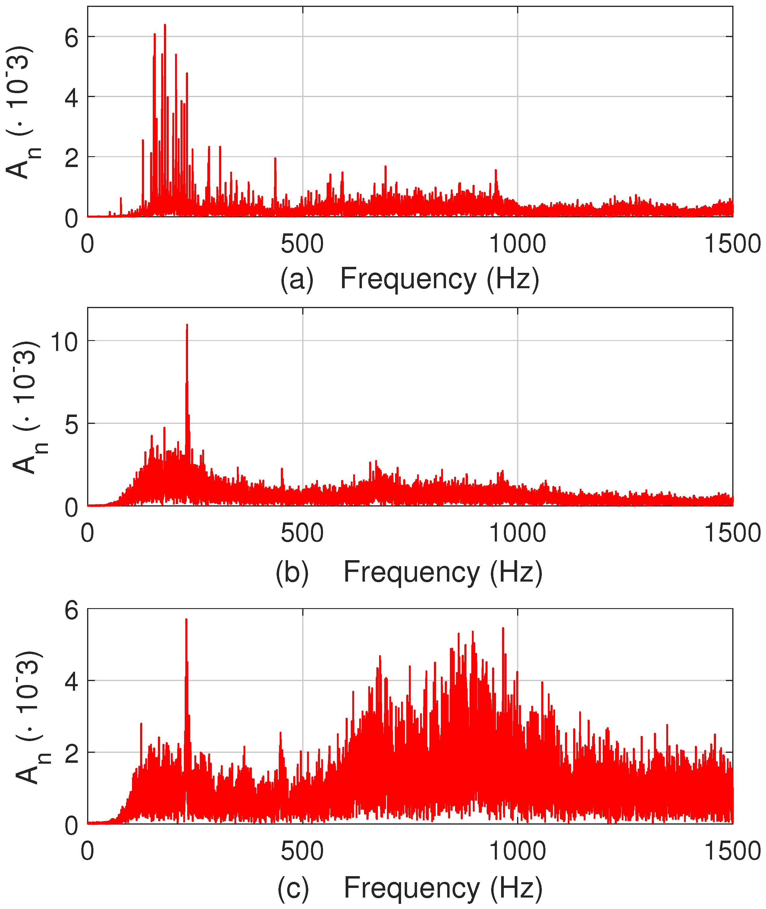
4.3. The Environmental Noise

In practical applications, the acoustic noise delivered by the rolling bearing is combined with the environmental noise, which causes the detection of faulty bearing to be adversely affected. Thus, it is important to include such a noise in the experimental validation of the proposed module. Indeed, in most works, the proposed monitoring techniques are tested considering healthy and faulty rolling bearings, which are connected to an electric motor and a load. However, the environmental noise is almost always neglected. Thus, in this work a different experimental setup is proposed. The wheel bearings of a car, which connect the wheel hubs to the constant velocity joints, are used as a test case in what follows. Such an application requires a highly reliable monitoring system, indeed also the driver safety can be affected by a damaged bearing. Moreover, such test case represents an harsh environment from the acoustic point of view, since the background noise is time-independent and it really depends on the driving conditions. As a consequence, the fault detection may be challenging. By means of an extra microphone patched on the car body over the front-left wheel, the sound of a moving vehicle was recorded in different scenarios. The frequency spectrum of such noise ($A_n$) was evaluated using Matlab and shown in Figure 8. More precisely, Figure 8a refers to the car started but not moving, Figure 8b to a straight with asphalt, and Figure 8c to a straight with gravel. It is worth noticing that such spectra are significantly populated up to 1 kHz, and that in every driving condition the environmental noise is far from being closed to a white noise.

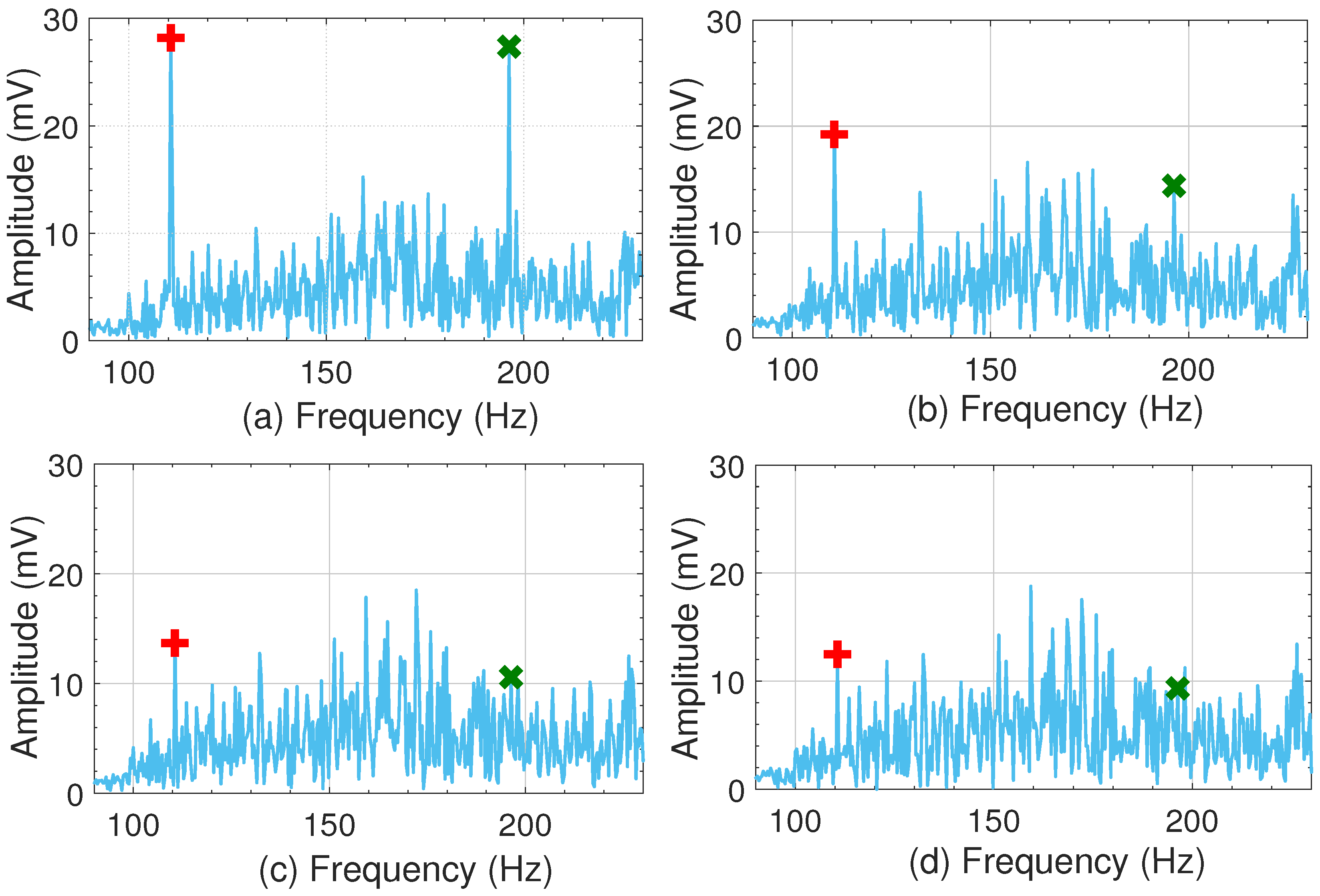
4.4. Two Tones Plus the Environmental Noise

Starting from the recorded environmental noise in the case of a car traveling along a straight with asphalt, two distinct tones were added in order to simulate the presence of an inner and outer race defect. More precisely, a tapered roller bearing [31] was considered and its dimensions exploited to evaluate the $BPFI$ and $BPFO$ fundamental frequencies, resulting in $BPFO$ = 1115 Hz and $BPFI$ = 197.6 Hz. The amplitude of such two tones was not constant, but different values were tested. In a such a way, it was possible to emulate different defect sizes. The average of the amplitude spectrum of the environmental noise in the range of 100 Hz to 1 kHz, named $A_{aver}$, was evaluated, and the amplitude of the two tones was defined according to

$$A_{tones}=A_{aver}\left(1+{10}^{\frac{A_{dB}}{20}}\right).$$

(11)

Thus, the environmental noise containing the two tones, which emulate a bearing with two defects, was reproduced closed to the proposed module, as shown in Figure 9, by means of a speaker. The module was configured so that $N_s=$ 16,384, $f_s=6$ kHz and the top flat window was exploited. Two ranges, centered around the $BPFO$ and $BPFI$ were considered, in particular $T{H}_{BPFO}=T{H}_{BPFI}$ = 10 mV and $f_{BPFO,e}-f_{BPFO,s}=f_{BPFI,e}-f_{BPFI,s}$ = 2 Hz. The frequency spectra evaluated by the modules itself are shown in Figure 10a–d for $A_{dB}$ and are equal to 40, 35, 30, and 25, respectively. As far as such a configuration is concerned, the proposed module is able to detect the tone at $BPFI$ if $A_{dB}\ge 30$ dB, and the one at $BPFO$ if $A_{dB}\ge 35$ dB. Indeed, the detection capability is strongly affected by the noise floor in the correspondence of the frequency ranges to be monitored.

5. Conclusions

This paper proposed a low-cost and Bluetooth connected module to detect defects in rolling bearings. The acoustic noise delivered by the bearing to be monitored is acquired by means of a MEMS microphone and sampled by a microcontroller, which also evaluates the frequency spectrum of the signal exploiting an optimized version of the Fast Fourier Transform algorithm for real data. The detection of defects is based on the exceeding of given thresholds in certain frequency ranges. If a fault is detected, the module notifies the central controller, thus reducing at the minimum the amount of transferred data and occupying the wireless channel only when it is required. The configuration parameters of the acquisition process, as well as the frequency ranges to be monitored can be modified on-the-fly through the wireless link. A prototype of the proposed system was realized, and the relative errors affecting the evaluation of the frequency spectrum were measured and discussed. It resulted that the use of a top-flat windowing function allows for an amplitude error within $\pm 0.6\%$ in the case of a single tone. Then, the wheel bearing of a vehicle was considered as a test case, and the environmental noise acquired in different driving scenarios. Such recorded noise was used as noise floor for the simulation of a faulty bearing, and the module successfully detected the damages, provided that the corresponding fundamental frequencies arose sufficiently from the environmental noise.

References

1. Holbert, K.E.; Lin, K.; Karady, G.G. Enhacement of electric motor reliability through condition monitoring. In Proceedings of the 5th IFAC Symposium on Power Plants and Power Systems Control, Kananaskis, AB, Canada, 25–28 June 2006; Volume 39, pp. 255–260. [Google Scholar] [CrossRef]
2. Caesarendra, W.; Kosasih, B.; Tieu, A.K.; Zhu, H.; Moodie, C.A.; Zhu, Q. Acoustic emission-based condition monitoring methods: Review and application for low speed slew bearing. Mech. Syst. Signal Process. 2016, 72–73, 134–159. [Google Scholar] [CrossRef]
3. Wang, D.; Tsui, K.; Miao, Q. Prognostics and Health Management: A Review of Vibration Based Bearing and Gear Health Indicators. IEEE Access 2018, 6, 665–676. [Google Scholar] [CrossRef]
4. Azeez, N.I.; Alex, A.C. Detection of rolling element bearing defects by vibration signature analysis: A review. In Proceedings of the 2014 Annual International Conference on Emerging Research Areas: Magnetics, Machines and Drives (AICERA/iCMMD), Kerala, India, 24–26 July 2014; pp. 1–5. [Google Scholar]
5. Piltan, F.; Prosvirin, A.E.; Jeong, I.; Im, K.; Kim, J.M. Rolling-Element Bearing Fault Diagnosis Using Advanced Machine Learning-Based Observer. Appl. Sci. 2019, 9, 5404. [Google Scholar] [CrossRef] [Green Version]
6. Wang, J.; Wang, J.; Du, W.; Zhang, J.; Wang, Z.; Wang, G.; Li, T. Application of a New Enhanced Deconvolution Method in Gearbox Fault Diagnosis. Appl. Sci. 2019, 9, 5313. [Google Scholar] [CrossRef] [Green Version]
7. Hou, J.; Wu, Y.; Gong, H.; Ahmad, A.S.; Liu, L. A Novel Intelligent Method for Bearing Fault Diagnosis Based on EEMD Permutation Entropy and GG Clustering. Appl. Sci. 2020, 10, 386. [Google Scholar] [CrossRef] [Green Version]
8. Hebda-Sobkowicz, J.; Zimroz, R.; Wyłomańska, A. Selection of the Informative Frequency Band in a Bearing Fault Diagnosis in the Presence of Non-Gaussian Noise—Comparison of Recently Developed Methods. Appl. Sci. 2020, 10, 2657. [Google Scholar] [CrossRef] [Green Version]
9. Lees, A.W.; Quiney, Z.; Ganji, A.; Murray, B. The use of acoustic emission for bearing condition monitoring. J. Phys. Conf. Ser. 2011, 305, 012074. [Google Scholar] [CrossRef] [Green Version]
10. Kilundu, B.; Chiementin, X.; Duez, J.; Mba, D. Cyclostationarity of Acoustic Emissions (AE) for monitoring bearing defects. Mech. Syst. Signal Process. 2011, 25, 2061–2072. [Google Scholar] [CrossRef]
11. Kim, J.; Kim, J.M. Bearing Fault Diagnosis Using Grad-CAM and Acoustic Emission Signals. Appl. Sci. 2020, 10, 2050. [Google Scholar] [CrossRef] [Green Version]
12. Orman, M.; Rzeszucinski, P.; Tkaczyk, A.; Krishnamoorthi, K.; Pinto, C.; Sułowicz, M. Bearing Fault Detection with the Use of Acoustic Signals Recorded by a Hand-Held Mobile Phone. In Proceedings of the International Conference on Condition Assessment Techniques in Electrical Systems (CATCON), Bangalore, India, 10–12 December 2015; pp. 252–256. [Google Scholar] [CrossRef]
13. Rubio, E.; Jáuregui, J.C. Experimental characterization of mechanical vibrations and acoustical noise generated by defective automotive wheel hub bearings. Procedia Eng. 2012, 35, 176–181. [Google Scholar] [CrossRef] [Green Version]
14. Lee, C.Y.; Huang, K.Y.; Hsieh, Y.H.; Chen, P.H. Optimal Intrinsic Mode Function Based Detection of Motor Bearing Damages. Appl. Sci. 2019, 9, 2587. [Google Scholar] [CrossRef] [Green Version]
15. Liu, W.; Zhao, T.; He, D.; Liu, D. DSP based module for processing vibration signals of rotation machinery. In Proceedings of the 2017 IEEE International Instrumentation and Measurement Technology Conference (I2MTC), Turin, Italy, 22–25 May 2017; pp. 1–6. [Google Scholar]
16. Kang, M.; Kim, J.; Jeong, I.; Kim, J.; Pecht, M. A Massively Parallel Approach to Real-Time Bearing Fault Detection Using Sub-Band Analysis on an FPGA-Based Multicore System. IEEE Trans. Ind. Electron. 2016, 63, 6325–6335. [Google Scholar] [CrossRef]
17. Jagannath, V.M.D.; Raman, B. WiBeaM: Wireless Bearing Monitoring System. In Proceedings of the 2007 2nd International Conference on Communication Systems Software and Middleware, Bangalore, India, 7–12 January 2007; pp. 1–8. [Google Scholar]
18. Esfahani, E.T.; Wang, S.; Sundararajan, V. Multisensor Wireless System for Eccentricity and Bearing Fault Detection in Induction Motors. IEEE/ASME Trans. Mechatron. 2014, 19, 818–826. [Google Scholar] [CrossRef]
19. Ramalingam, I.; Annamalai, S.; Vaithiyanathan, S. Fault diagnosis of wind turbine bearing using wireless sensor networks. Therm. Sci. 2017, 21, 523–531. [Google Scholar] [CrossRef] [Green Version]
20. Lu, S.; Zhou, P.; Wang, X.; Liu, Y.; Liu, F.; Zhao, J. Condition monitoring and fault diagnosis of motor bearings using undersampled vibration signals from a wireless sensor network. J. Sound Vib. 2018, 414, 81–96. [Google Scholar] [CrossRef]
21. Huang, Q.; Tang, B.; Deng, L.; Wang, J. A divide-and-compress lossless compression scheme for bearing vibration signals in wireless sensor networks. Measurement 2015, 67, 51–60. [Google Scholar] [CrossRef]
22. Feng, G.; Zhao, H.; Gu, F.; Needham, P.; Ball, A. Efficient implementation of envelope analysis on resources limited wireless sensor nodes for accurate bearing fault diagnosis. Measurement 2017, 110, 307–318. [Google Scholar] [CrossRef]
23. Randall, R.B.; Antoni, J. Rolling element bearing diagnostics—A tutorial. Mech. Syst. Signal Process. 2011, 25, 485–520. [Google Scholar] [CrossRef]
24. Brandlein, J.; Eschmann, P.; Hasbargen, L.; Weigand, K.B. Ball and Roller Bearings: Theory, Design and Application; Wiley: Hoboken, NJ, USA, 1999. [Google Scholar]
25. Kumar, B.P. Digital Signal Processing Laboratory; Taylor and Francis Group: Abingdon, UK, 2010. [Google Scholar]
26. Soni, M.; Kunthe, P. A General Comparison of FFT Algorithms. Pioneer Journal of IT and Management. 2011. Available online: http://pioneerjournal.in/conferences/tech-knowledge/12th-national-conference/3625-a-general-comparison-of-fft-algorithms.html (accessed on 13 August 2020).
27. Sundararajan, D. The Discrete Fourier Transform; World Scientific: Singapore, 2001; Available online: https://www.worldscientific.com/doi/pdf/10.1142/4610 (accessed on 30 June 2020).
28. Harris, F.J. On the use of windows for harmonic analysis with the discrete Fourier transform. Proc. IEEE 1978, 66, 51–83. [Google Scholar] [CrossRef]
29. ARM. Cortex™-M3, Technical Reference Manual; ARM: Cambridge, UK, 2005. [Google Scholar]
30. Bluetooth Special Interest Group. Bluetooth Core Specification; Bluetooth Special Interest Group: Kirkland, WA, USA, 2019. [Google Scholar]
31. NTN Bearing Corporation. 4T-30207 Tapered Roller Bearing; NTN Bearing Corporation: Osaka, Japan, 2015. [Google Scholar]
Figure 1. Flowchart of the optimized algorithm for the frequency spectrum evaluation.
Applsci 10 05645 g001
Figure 2. Number of operations (sums and multiplications) required to evaluate the discrete fast Fourier transform (DFFT) according to the classical algorithm (dashed-dot line) and to the optimized one (continuous line).
Applsci 10 05645 g002
Figure 3. Scheme of the hardware blocks required by the proposed solution.
Applsci 10 05645 g003
Figure 4. The i-th and the j-th range are shown, alongside their thresholds ( T H i , T H j ) and frequency intervals. In such a case, a fault is detected in the j-th range.
Applsci 10 05645 g004
Figure 5. Relative error affecting the (a) fundamental frequency and (b) amplitude of the input sinusoidal signal, when no windowing is used.
Applsci 10 05645 g005
Figure 6. Relative error affecting the (a) fundamental frequency and (b) amplitude of the input sinusoidal signal, when the order 2 Hann window is used.
Applsci 10 05645 g006
Figure 7. Relative error affecting the (a) fundamental frequency and (b) amplitude of the input sinusoidal signal, when the top flat window is used.
Applsci 10 05645 g007
Figure 8. Frequency spectrum of the environmental noise in the proximity of the left front wheel when (a) the car is started but not moving, (b) the car is traveling along a straight with asphalt at 60 km/h, and (c) the car is traveling along a straight with gravel at 20 km/h. The amplitude of the time-domain signal was normalized between [−1,1].
Applsci 10 05645 g008
Figure 9. Test setup including the developed module and the speaker that reproduces the synthesized sound.
Applsci 10 05645 g009
Figure 10. Frequency spectra evaluated by the developed module in case of 2 tones added to the environmental noise, for (a) A d B = 40 dB, (b) A d B = 35 dB, (c) A d B = 30 dB, and (d) A d B = 25 dB. The plus markers refer to the B P F O tone and the cross ones to the B P F I tone.
Applsci 10 05645 g010