Article

On Modeling and Simulation of Resource Allocation Policies in Cloud Computing Using Colored Petri Nets

by
Stavros Souravlas
1,*,†,
Stefanos Katsavounis
2,† and
Sofia Anastasiadou
3
1
Department of Applied Informatics, University of Macedonia, 54636 Thessaloniki, Greece
2
Department of Production and Management Engineering, Democritus University of Thrace, 67150 Xanthi, Greece
3
Department of Early Childhood Education, University of Western Macedonia, 53100 Florina, Greece
*
Author to whom correspondence should be addressed.
These authors contributed equally to this work.
Appl. Sci. 2020, 10(16), 5644; https://doi.org/10.3390/app10165644
Submission received: 20 July 2020 / Revised: 9 August 2020 / Accepted: 11 August 2020 / Published: 14 August 2020
(This article belongs to the Special Issue Recent Advances in Sustainable Process Design and Optimization)

Abstract

:
The Petri net (PN) formalism is a suitable tool for modeling parallel systems due to its basic characteristics, such as synchronization. The extension of PN, the Colored Petri Nets (CPN) allows the incorporation of more details of the real system into the model (for example, contention for shared resources). The CPNs have been widely used in a variety of fields to produce suitable models. One of their biggest strengths is that their overall philosophy is quite similar to the philosophy of the object-oriented paradigm. In this regard, the CPN models can be used to implement simulators in a rather straightforward way. In this paper, the CPN framework is employed to implement a new resource allocation simulator, which is used to verify the performance of our previous work, where we proposed a fair resource allocation scheme with flow control and maximum utilization of the system’s resources.

1. Introduction

The cloud provides a variety of resources for users based on their requirements. Each job generated by a user in the cloud has some resource requirements. Thus, one important aspect of cloud computing is the design of an efficient resource allocation scheme. A second but equally important aspect is the evaluation of the different models of the cloud resources allocation and usage. It is common knowledge that it is very difficult to experiment on real cloud environments. Moreover, this experimentation is rather costly. Thus, many works focus on the design of simulation frameworks for cloud computing. Necessarily, these efforts can cover only some details of the overall cloud implementation, but they can serve as important experimentation tools. In this work, we extend our previous work [1] and discuss these aforementioned aspects—first, we briefly discuss our previous resource allocation scheme, to make the paper self-contained and to help the reader understand its details. Then, we show how to implement our own simulator, which is based on the Colored Petri Net formalism and incorporates the the main ideas of our resource allocation scheme.
The problem of resource allocation in the cloud is a challenging one, as the set of user jobs have much different requirements [2,3]. Due to to the heterogeneity of both the available resources (like CPU, bandwidth or memory) and the jobs themselves (for example, other jobs are CPU-intensive while others are memory-intensive), the problem of distributing the resources in a fast and fair way while regulating the resource utilization, becomes rather complex. By fairness, we actually mean a measure of how well the resource allocation is balanced among the users jobs, but also satisfy their needs to the maximum extent.
As the cloud usage is getting more and more intense, specifically due to the numerous big data applications running over the cloud [4,5] lot of effort has been focused on the resource allocation problem. The basic quality criteria for a good resource allocation technique, as described in the literature, are the minimization of the resource allocation cost, the overall system utilization and the job execution time. The techniques developed use different approaches in order to address these three metrics. In Reference [6], the authors treat the problem of resource allocation as an optimization problem and aim at reducing the total cost while they introduce the idea of increasing the overall reliability. The reliability is modeled on a per virtual machine (VM) basis and depends on the number of failures per VM.
In Reference [7] the authors divide the resource allocation technique into two phases: an open market-driven auction process followed by preference-driven payment process. When a user requests multiple resources from the market, the provider allocates them based on the user’s payment capacity and preferences. The users pay for the VMs based on the quantity and the duration used. The authors also aim at minimizing the total cost and allocate the resources in an efficient manner. Another work that mainly focuses on the total cost and utilization maximization was proposed by Lin et al. [8], where the authors propose a threshold-based strategy for monitoring and predicting the users’ demands and for adjusting the VMs accordingly. Tran et al. [9] present 3-stage scheme that allocates job classes to machine configurations, in order to attain an efficient mapping between job resource requests resource availability. The strategy aims at reducing the total execution time as well as the cost of allocation decisions.
Hu et al. [10] implemented a model with two interactive job classes to determine the smallest number of servers required to meet the service level agreements for two classes of arrived jobs. This model aims at reducing the total cost of resource allocation.
Khanna and Sarishma [11] presented RAS (Resource Allocation System), a dynamic resource allocation system, to provide and maintain resources in an optimized way. RAS is organized into 3 functions—Discovery of resources, monitoring of resources and dynamic allocation. The main goal is to achieve high utilization. The total resource allocation cost is not taken into account and the VM having minimum resource requirements suffer lower delay. In case of similar requirements, the VM have a random, equal waiting time.
Two strategies focusing on the total execution time are found in Reference [12,13]. Saraswathi et al. present a resource allocation scheme, which is based on the job features. The jobs are assigned priorities and high priority jobs may well take the place of jobs with low priorities. In Reference [13], the authors use the concept of “skewness” to measure the unevenness in the multidimensional resource utilization of a server. Different types of workloads are combined by minimizing the skewness and the strategy aims at achieving low execution times by balancing the load distributed over time. Table 1 summarizes the discussion so far, by indicating the metrics considered by the papers described.
Generally, the simulators have an important role in the development of every software application. When a researcher tries to design a resource allocation strategy for the data centers of a cloud, he focuses on the aspects mentioned above, that is, the minimization of the resource allocation cost, the overall system utilization and the job execution time. A well-developed simulator will help the researcher to grasp the main issues and challenges of the problem like the resource allocation strategy to be used, the choice of the basic cloud resources (in an initial stage, it is necessary to keep the most important resources, so that the simulator can be tested easily), and the other factors that are important (for example, an input rate regulation policy, as will be discussed in the next section). The simulator will provide answers to questions involving the effectiveness of resource utilization, or the “fair” distribution among the competitive user jobs. Also, it may prove that an allocation strategy performs better under certain job input rates, which are regulated based on the service time of the resource allocations over the cloud. In the remaining of this section, we briefly discuss a few of the typical cloud simulators found in the literature, which include modules for resource allocation based on a certain policy. A detailed presentation of the existing cloud simulators can be found in a very recent comprehensive work presented by Mansouri et al. [14].
One of the first cloud simulators, was introduced by Calheiros et al. [15] and was named CloudSim. This simulator was the basis for the development for a number of other simulating tools (examples include References [16,17,18,19,20]). CloudSim supports allocation provisioning at two levels—(1) host level and (2), at the Virtual Machine level. At the host level, decisions are taken regarding the percentage of the processing power of each cort that will be allocated to each VM. At the VM level, the VM assigns a constant percentage of the processing power to the individual jobs within the VM. Sqalli et al. [21] presented UCloud, which was developed for usage in a university environment. The model combines public and private clouds and the resource allocation policy is based on information like performance monitoring or security management. The  DISSECT-CF (DIScrete event baSed Energy Consumption simulaTor for Clouds and Federations) simulator presented by Kecskemeti [22] includes a module that can track major resource conflicts (like CPU or bandwidth) to take decisions regarding the resource sharing. These decisions are enhanced by a tool for performance optimization, as far as the resource distribution is concerned.
Tian et al. [23] introduced their simulator named CloudSched simulator. The simulator includes resource allocation policies in the cloud, which are built upon the consideration of the main resources like CPU, memory and disk, and network bandwidth. The approach (like the one proposed in this work) also makes use of the average service time, the job input rate and the service time to take decisions on the resource allocation. However, it does not include a fairness mechanism and it does not separate the user jobs into different classes, based on their dominant resource needs, as does our strategy.
In Reference [24], the authors introduced SCORE, which includes a resource allocation module. To create the model for the generated jobs, SCORE takes into account the job inter-arrival time, the job duration and the resource usage, that is the amount of CPU and RAM that every job needs to consume. Again, the module is not equipped with a fairness strategy and it does not take into account the nature of each job, that is, some of the jobs are CPU intensive while others are memory intensive. The simulator presented by Gupta et al. [25] also includes a resource management module. This module consists of a set of schemes. The workload management is one of these schemes and its purpose is to decide where to accommodate the workload. An optimization workload management algorithm may be used to select among a set of feasible solutions. Also, a control based workload management algorithm can be used to control the system. This type of management can closely track the performance parameters (for example job service time) of jobs in order to regulate the workload input rate. A researcher can examine these resource allocation algorithms with different workload distributions.
The Petri Net and Colored Petri Net formalism have been widely used in the literature, in numerous fields [26,27]. Only a few are mentioned here: A few applications to mention here include pipeline-based parallel processing [28], grid computing applications [29,30] or even traffic control [31]. In this paper we use an extension of Petri Nets, the Colored Petri Nets (CPN) to extend our previous work [1], which proposed a resource allocation method, to maximize the resource utilization and distribute the system’s resources in a fast and fair way. Compared to the other resource allocation schemes found in the literature, this work introduces the control flow control mechanism based on the available resources and the careful analysis of the dominant demands of each job. Also, the metric it uses for performance evaluation is the system utilization (see Table 1 for comparisons to other schemes), although its execution time could also be used since it is proven to be linear, as will be discussed is Section 3. In this work, we capture the ideas of our previous work and use them to implement a CPN model for resource allocation in the cloud. This model is the basis for the implementation of our CPN-based resource allocation simulator (will be referred to as CPNRA (Colored Petri Net-based Resource Allocator). This simulator is used to verify and evaluate the performance of our resource allocation scheme. The advantages of the proposed model is that it is deadlock free and can be executed in linear time. Moreover, because it is organized in an hierarchical manner, it can easily be expanded for larger systems (larger number of users or available resources) only with minor changes. This is one of its biggest strengths.
The remaining of this work is organized as follows—Section 2 briefly describes the resource allocation model. More details can be found in Reference [1], but we present the basic ideas here, so that the paper is standalone. Section 3 presents some CPN preliminaries which are necessary for the reader to understand the model and then shows how we translated the resource allocation model to a CPN model. In Section 4, we explain how the simulator executes giving a concrete example and then we present our experimental results. Section 5 concludes this paper and presents aspects for future research.

2. Resource Allocation Model

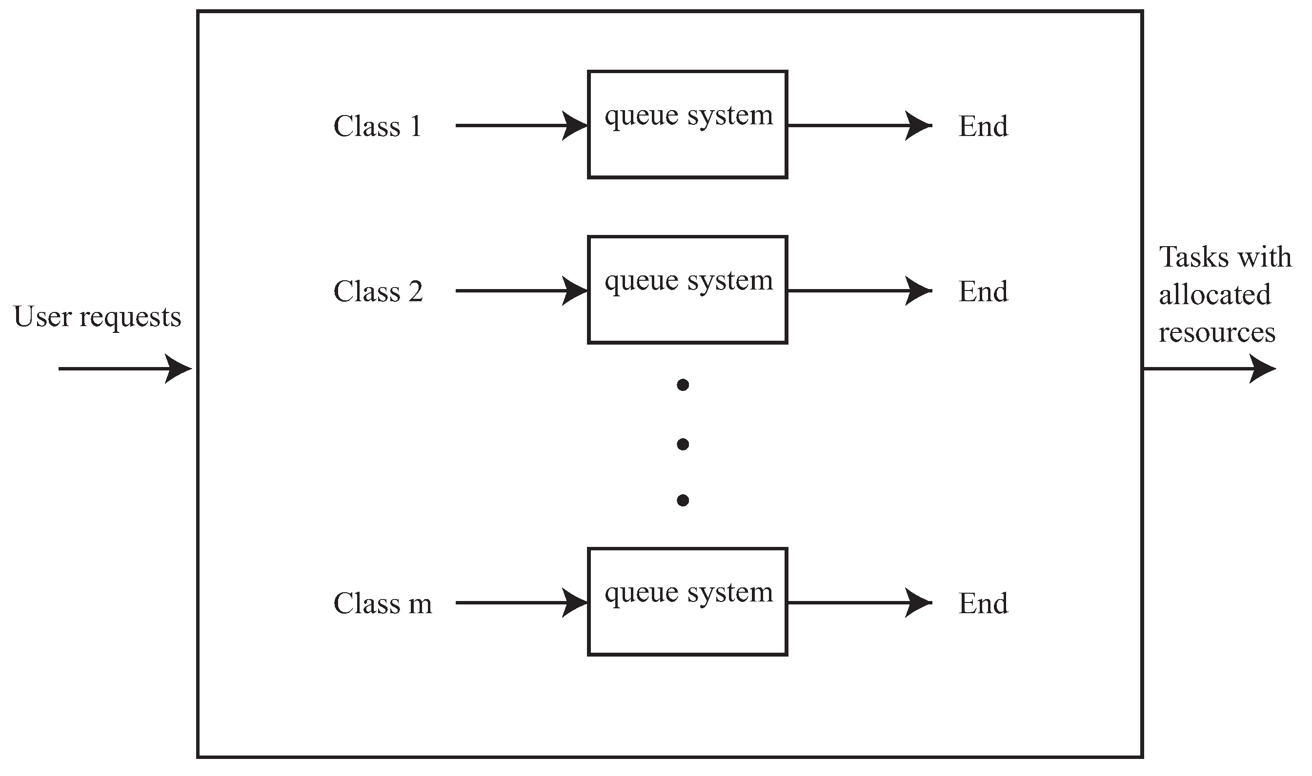
Consider a set S = { 1 , , m } of m available resources, where T r is the total amount of a resource r available in the cloud. In our allocation model, the resources are considered as servers. Each resource type r is modeled as a single server S r , and each server has a single queue Q r of user jobs that require the specific resource. The queue lengths are considered large enough to accommodate all the possible user requests per resource. The jobs enter a queue Q r to request a resource type according to a Poisson arrival process with rate λ r . The service time (the time required for a job to obtain a certain resource) is exponential with mean 1 / μ . A cloud has an infinite number of users and each user executes a number of jobs. Each job is described by its demand vector V i = { V i 1 , V i 2 , V i m } . The demand vector shows the amount of each resource demanded by each job. A job’s job dominant resource, is the most necessary resource for this job. For example, some jobs are CPU-intensive, while others require more memory. This notion has been introduced in a number of papers (for example, see References [32,33]). The dominant server queue (DSQ) is the queue of the dominant resource server. All the jobs requiring a dominant resource enter the DSQ before entering any other queue to ask for other resources. In the example of Figure 1, the DSQ is Q 1 . The remaining queues correspond to non-dominant resources.
A vector in the form K = ( K 1 , K 2 , , K m ) expresses the cloud’s state. Here, K is the amount of available resources in every server. Let us consider the conditional probability of moving from state K to K , denoted as p ( K , t + δ | K , t ) , where δ is a very short period, enough to accommodate only one change of state. The overall probability of reaching a state K is: [34]
p ( K 1 , K 2 K m ) = p 1 ( K 1 ) · p 2 ( K 2 ) · · p m ( K m )
where
p j ( K j ) = p j K j ( 1 p j ) ,
with
p j = λ j μ j 1 ,   the utilization of a resource server .
Let us consider a system has the 3 most important resources, that is, CPU, RAM, and disk. A resource allocator (see Figure 2) is used; the resource allocator is a central system that handles a queue system. Generally, the resource allocator has m queue systems or classes, each having a structure similar to the one shown in Figure 1. A class is characterized by the dominant resource. Each class has m queues, one for each resource. For our example, m = 3 . Thus, the total number of queues in the system m 2 . Obviously, the dominant resource is different for each queue system and each system handles and allocates a percentage of the overall available resources. We use b i to refer to this percentage for each queue. In the example of Figure 1, b 1 is the percentage of the dominant queue (in our example Q 1 ) and b 2 , b 3 are the percentages for the remaining queues ( Q 2 and Q 3 for our example).
When a job requires resources, its dominant resource is examined and it is assigned to the proper queue system, the one with the dominant resource as DSQ. Thus, a job requests resources starting from DSQ and then it “moves” accross the other queues to request the remaining resources. Then, it may “return” back to DSQ to request more resources. Mathematically, for the queue system of Figure 1, this behavior is modeled by the following equations:
λ 1 = λ + ( μ 2 + μ 3 ) b 1 λ 2 = b 1 λ 1 λ 3 = b 2 λ 2 ,
where λ denotes the total number of rate of all the jobs with Q 1 as their DSQ. The  b j ’s have to be regularly recalculated, as resources are allocated and de-allocated.
Therefore, by employing a queuing system, our resource allocation scheme is able to estimate the maximum job arrival rate that the system can afford.
To distribute the resources in a fair way, our scheme introduces a m a x j o b fair policy, which initially considers the maximum number of jobs based on the demands on the dominant resource. Let us define U = { U 1 , , U n } as the set of n users that content for the dominant resource r ^ . The users are sorted by increasing order of their demands for the dominant resource into vector V r ^ and then U i max , the maximum number of job assigned to each user is computed as follows:
U i max = T r ^ V i r ^ , for all users i .
Then, we find the sum of all the jobs computed in the first step, N = i = 1 n T r ^ V i r ^ , and we find the fair resource allocation factor f for each of these jobs as follows:
f = T r ^ N .
Finally, we use the fair resource allocation factor to compute the resources allocated fairly to each user i, F i as follows:
F i = f × U ( n + 1 i ) max .
Let us use an example to illustrate the process described. Assume that 4 users content for their dominant resource, CPU, and the cloud system has 18 CPUs available and their demands are: 4 CPUS for U 1 , 9 CPUs for U 2 , 6 CPUs for U 3 and 5 CPUs for U 4 . By sorting in ascending order, we have: V = [ U 1 = 4 , U 4 = 5 , U 3 = 6 , U 2 = 9 ] . From (4), we obtain that U 1 max = 18 4 = 4.5 , U 2 max = 18 5 = 3.6 , U 1 max = 18 6 = 3 , and U 4 max = 18 9 = 2 . The sum of these jobs is N = 4.5 + 3.6 + 3 + 2 = 13.1 jobs. Then f = 18 13.1 = 1.374 . Thus, from (6), we have:
F 1 = 1.374 × U 4 max = 1.374 × 2 = 2.748 , F 2 = 1.374 × U 3 max = 1.374 × 3 = 4.122 , F 3 = 1.374 × U 2 max = 1.374 × 3.6 = 4.97 , and F 4 = 1.374 × U 1 max = 1.374 × 2 = 6.18 .
Since the values [ F 1 , F 2 , F 3 , F 4 ] correspond to users [ U 1 , U 4 , U 3 , U 2 ] (recall that the users have been sorted based on their requests, from Step 1). Thus, U 1 will get 3 CPUs, U 2 will get 6 CPUs, U 3 will get 5 CPUs and U 4 will get 4 CPUs.
To conclude, our resource allocation policy first examines the job arrival rate that the system can afford by solving a system of equations like the one in Equation (4) and then it applies Equations (5)–(7) to fairly distribute the resources. In cases when the requesting jobs arrival rate is such that the system cannot handle, then the system reduces the resources assigned to each job by Equations (5)–(7), until the rates are regulated to affordable values.

3. The CPN Model

In this section we present the CPN model, which is the basis for the implementation of our simulator. The CPN model is composed of one “core” for each queue member of a queue system. The cores have the same structure and procedures described in this section, but they differ only on the resource which is the dominant one. All the cores are executed in parallel and there is no need to interconnect them. This increases the allocation speed. In the following subsections, we describe the cores in detail, and then we present deadlock analysis. However, we initially have to provide the necessary background of the CPN formalism.

3.1. The CPN Formalism

The CPN formalism is an extension of the basic PN formalism, which has been implemented to overcome two important challenges—(1) The typical PN formalism does not distinguish between the tokens, in other words all the tokens have the same meaning and they are used to represent a system’s state. However, in most of the cases, a system’s entities may have some common attributes but the values of these attributes differ from entity to entity, while these values are of high importance for the study of the system. and (2) The typical PN formalism does not bother about the actual timing of events that may change the system’s state, but only for the sequence of these events. This is a disadvantage, when researchers try to model systems which have inherited timing attributes. In the remaining of this subsection, we discuss the data and timing extensions of the PN formalism, which have resulted to the CPN. Whenever necessary, we will give definitions regarding other important elements of Petri Nets. Also, we will discuss another useful extension, the guarding expressions, which generate the conditions under which an event can occur at a certain time. The Colored Petri Nets, not only take the timing factor into account, but also they use the guards to define conditions under which an event can (or cannot) occur at a certain time.

3.1.1. Data Extensions

In this paragraph, we discuss the first extension of Petri nets, where the tokens are distinguished through the assignment of specific values to each one of them. This value is named color, hence the name Colored Petri nets.
When modeling a system as a simple Petri net, the system’s elements are represented by tokens, places, and transitions (definitions for the places and transitions are given later in this paragraph). A  token is a dynamic element of a Petri net, and it is used to define the network’s state. A token can model an object or a set of objects and also states and conditions. For example, in a cloud system a token may model a user job that is CPU intensive (requires more CPU processing resources) while another token may model a memory intensive job (requires more memory). In a simple Petri net, it is impossible to distinguish between these two tokens and describe their attributes. With the CPN formalism, each token carries a value. Other token attributes may include the arrival time, the mean service time, and so forth. We can describe a job with the five attributes: Job_Id, Job_Priority, Arrival_Time, Service_Time, and Type_of_Resources_Requested, as will be discussed when we describe our model. Then, each token will have its own values, like:
1, 1, 10, 50, [1,1,1]   or   2, 1, 20, 60, [1,1,0]
To describe the network structure and the behavior of CPNs in a formal way, we need to define the notions of places and transitions. A place is represented by circles and they are the containers of tokens. The number and type of tokens inside a place define a network’s state. In other words, a place represents a system’s state, which is defined by the number and type of tokens it contains. For example, if a place has two jobs <1, 1, 10, 50, [1,0,0]> and <2, 1, 20, 60, [1,0,0]> then it represents a state where two user jobs have been generated, one with Id = 1, Priority = 1, generated at time = 10, scheduled to be served after 50 time units, and requesting only the dominant resource and another one with Id = 2, Priority = 1, generated at time = 20 and scheduled to be served after 60 time units, and also requesting only the dominant resource. A monitor, which is transparent to the core generates these tokens (see Section 4.1). A place can only accept tokens of one form: this can include a certain type of token (for example job tokens) or a union of tokens (tokens which are formed by the union of two or more tokens).
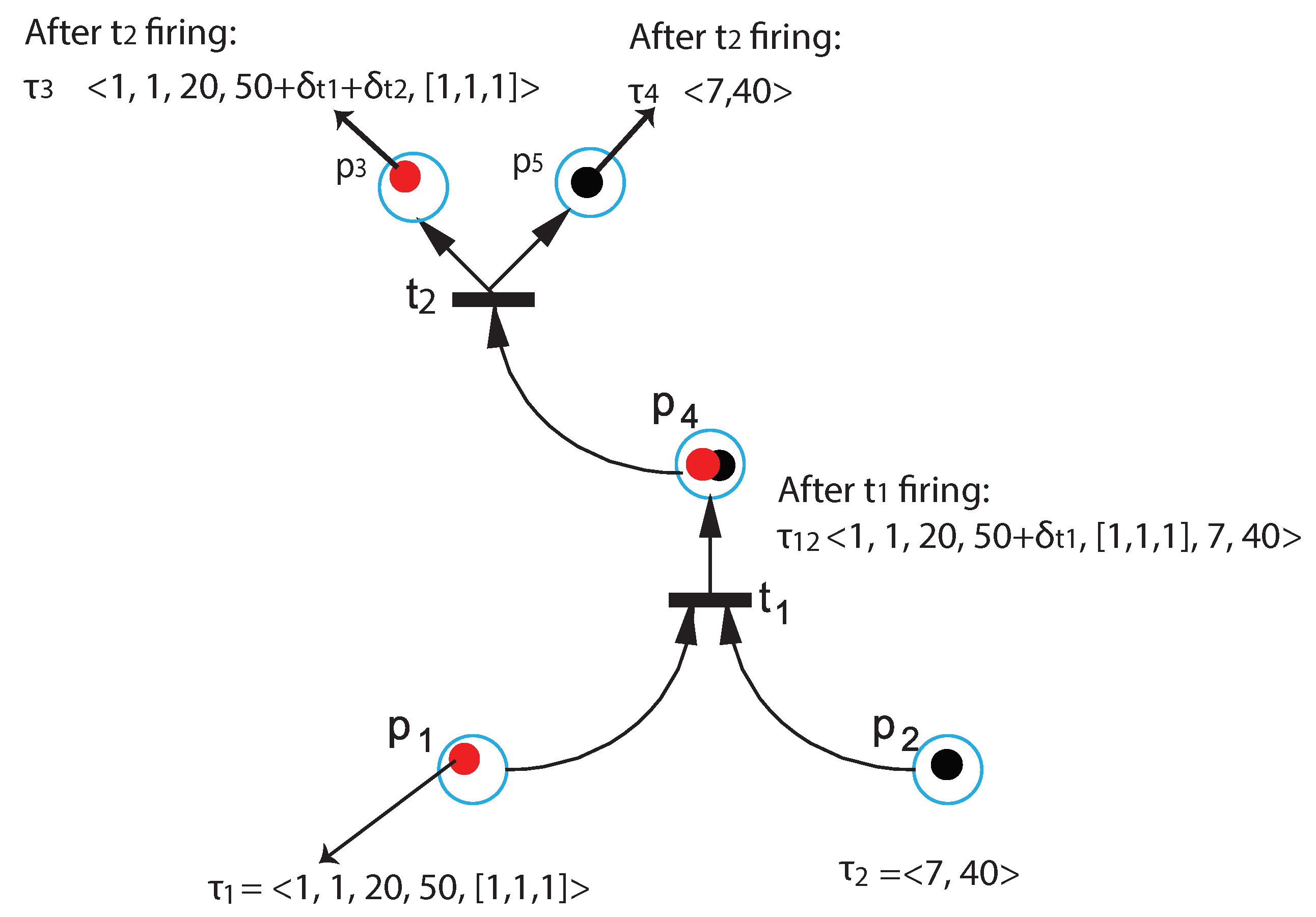
A transition represents an event that, whenever triggered, it may change the system’s state, that is, the system may transition from one state to another. Transitions are represented by rectangles. Generally, we use the verb “fire” to indicate that an event has occured. In order for a transition to fire, all its conditions must be satisfied. In this case, we say that the transition is enabled. We use the example of Figure 3 to show these considerations. In this figure (as well as in all the others), the types of tokens are colored for clarity of the presentation.
Figure 3 shows 5 positions, p 1 and p 3 which accommodate only red tokens and p 2 , p 5 which accommodates only black tokens, and  p 4 which accommodates red-black tokens (union of reds and blacks). Also, there is one transition t 1 that is fed by p 1 and p 2 and transition t 2 which is fed by p 4 . Transition t 1 is enabled when its inputs p 1 , p 2 have at least one token. The inputs to a transition are indicated by arrows originating from one or more place to this transition. Thus, the existence of at least one token to the transition’s input place forms the condition that must hold before it fires.
When firing, a transition will change the system’s state. Then, one token from each input place is removed and placed to the transition’s output place, in our example p 4 . In the context of CPN, the two different types are united. If we consider two tokens τ 1 , τ 2 as a set of elements or values in the form { τ 1 _ V a l u e 1 , τ 1 _ V a l u e 2 , τ 1 _ V a l u e N } and { τ 2 _ V a l u e 1 , τ 2 _ V a l u e 2 , τ 2 _ V a l u e N } then the new token is the union of the two sets:
τ 12 = { τ 1 _ V a l u e 1 , τ 1 _ V a l u e 2 , τ 1 _ V a l u e N } { τ 2 _ V a l u e 1 , τ 2 _ V a l u e 2 , τ 2 _ V a l u e N } = { τ 1 _ V a l u e 1 , τ 1 _ V a l u e 2 , τ 1 _ V a l u e N , τ 2 _ V a l u e 1 , τ 2 _ V a l u e 2 , τ 2 _ V a l u e N } .
In Figure 3, notice the new token τ 12 in place p 4 . It is the union of the set of values of τ 1 and  τ 2 . Its color is red-black, to denote this union in a pictorial manner. Now, t 2 and t 3 are also enabled, When  t 2 is also enabled. When it fires, the token τ 12 is split again and its red part only moves to p 3 as a new token τ 3 (recall that p 3 accommodates only red tokens) while its black part only moves to p 4 as a new token τ 4 (recall that p 4 accommodates only black tokens).
Now, we can typically define a CPN network. It is composed of 4 elements:
1.
A set of places P
2.
A set of transitions T
3.
An input function I
4.
An output function O
The input and output function relate places to transitions. An input function I is a mapping from a set of places to a transition t i . It is denoted by I ( t i ) and the set of places is called input places for the transition. As mentioned in our example, I t 1 = { p 1 , p 2 } . The output function O is a mapping from a transition to a set of places. It is denoted by O ( t i ) and the set of places is called output places for the transition. As mentioned in our example, O t 1 = { p 4 } . The tokens τ i are distinguished according to the CPN formalism, as described above.
Then, a Colored Petri Net C is typically defined as a quadruple of the form C = { P , T , I , O } , where:
P = { p 1 , p 2 , , p n , } is a finite set of places, n 0
T = { t 1 , t 2 , , t n , } is a finite set of transitions, n 0
R T is an input function from a subset of places R to a transition of set T, and 
T R is an output function from a transition of set T to a subset of places R.
Finally, we define the marking of a network C as the number and type of all the tokens residing in all the places at a certain time. An initial marking is necessary when we start the simulation engine. This initial marking defines the initial system conditions.

3.1.2. Timing Extensions

Now, we address the second extension of Petri nets, where the transitions are not timeless but timed. The provision of time gives our model the opportunity to describe the temporal details of a system in a precise manner. The approach combines three characteristics—(1) Each token carries one time stamp, a timing value used to determine the firing time of the transitions fed by the place this token is located (2) a transition may fire and produce new tokens with a delay, and (3) a guard expression can be used when we need to assign conditions regarding the time of firings. When we consider time, there is always a global clock for keeping the time. Time is usually advances in time units and not in real time metrics (hours, minutes, seconds, etc.). For transition firings, it is a common practice to add a delay, which is analogous the time required for the system changes to take effect.
To determine the firing time of a transition, we first examine all the input places and from each place, we find the token with a minimal time stamp (that is, the next token to leave this place). In case of a draw between time stamps residing in a place, the system chooses the one with the smaller Job_Id. Thus when a transition has b input places, we take into account b tokens, one token with the minimum time stamp from each of these places. Then, the firing time is equal to the maximum of the selected time stamps, t i max indicating that the last condition required to enable transition t i became true at time t i max . This procedure will be clarified with an example in Section 3.2.4, where the firing time of our model is described.
When the firing time is determined, a delay time stamp determines the time of birth for the new token in its next place (the transition’s output place). In other words, the time stamp of the newly produced token is the sum of the determined firing time and the introduced delay. The delay is an indication that the proper time has elapsed before the new token is produced and located to its new place. This means that we have to take into account the time required for an event to complete and affect the system’s state.

3.1.3. Guarding Expressions

There are cases where multiple transitions can be enabled at a time. In this case, there must be some type of referee, who decides which transition to fire first. In the CPN, the role of the referee is given to a special type of expressions called guards or guarding expressions. In this context, the guards are written in parentheses. In Section 3.2.3 we describe the guard expressions that define the necessary conditions for our model and provide details on how they operate.
The notions and ideas described in this paragraph will be used next, in the description of our CPN based model for resource allocation over the cloud.

3.2. The CPN Model

In this subsection we present the CPN model, which is the basis for the implementation of our CPNRA simulator. The CPN model is composed of one “core” for each queue member of a queue system. The cores have the same structure and procedures described in this section, but they differ only on the dominant resource. All the cores are executed in parallel and there is no need to interconnect them. This increases the allocation speed. In the following subsections, we describe the cores in detail, and then we present deadlock analysis.

3.2.1. The Core of Queue Members of a Queue System

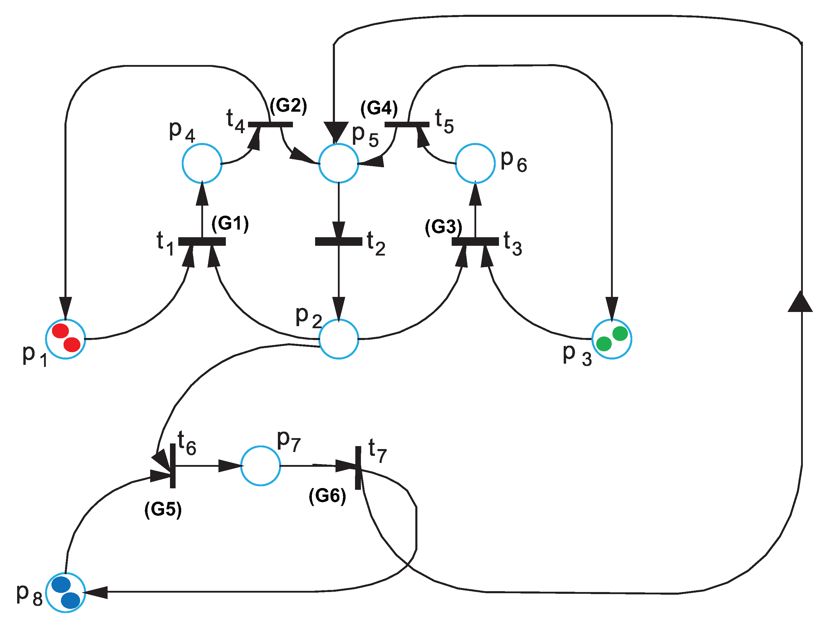
Our resource allocation scheduler is composed of m queue systems, each having m queues. In this subsection we will describe the core for the DSQ (the first queue, Q 1 ) of a queue system. Figure 4 shows this core. Inside each core a number of transitions which involve the DSQ are implemented. These transitions are symbolized by T 1 x and T x 1 , where x 1 , x i n [ 2 , m ] , and are described as follows:
(1)
T 12 : The transition from the DSQ Q 1 to Q 2 , in other words, the dominant resources have been allocated to a job, which then applies for resources from server S 2 , thus it enters its queue.
(2)
T 13 : The transition from the DSQ Q 1 to Q 3 , in other words, the dominant resources have been allocated to a job, which then apply for resources from server S 3 , thus it enters its queue.
(3)
T 21 : The transition from the Q 2 to the DSQ; the requested resources have been allocated from S 2 to a job, that returns to request extra resources from the DSQ, thus it re-enters its queue.
(4)
T 31 : The transition from the Q 3 to the DSQ; the requested resources have been allocated from S 3 to a job, that returns to request extra resources from the DSQ, thus it re-enters its queue.
The places and transitions of the DSQ core are given below:
  • Places
  • p 1 : Jobs requesting DSQ resources
  • p 2 : Processing of next job request
  • p 3 : Jobs requesting resources from server Q 2
  • p 4 : Fair allocation policy over DSQ
  • p 5 : All ToRRs (Type of Resources Required, see Section 3.2.2 where the token structure is described) updated, Next job selection
  • p 6 : S 1 Fair allocation policy over Q 2
  • p 7 : S 2 Fair allocation policy over Q 3
  • p 8 : Jobs requesting resources from server Q 3
  • Transitions
  • t 1 : Compute DSQ resources to be allocated for the job in a fair way
  • t 2 : Process the next job’s allocation request,
  • t 3 : Compute Q 2 resources to be allocated for the job in a fair way
  • t 4 : Allocate DSQ resources, update ToRRs accordingly
  • t 5 : Allocate Q 2 resources
  • t 6 : Compute Q 3 resources to be allocated for the job in a fair way
  • t 7 : Allocate Q 3 resources
One should notice the hierarchy behind this model: each of the queues is implemented with a subset of places and transitions and also, the queues have some places and transitions in common. For example, the DSQ is implemented with places p 1 and p 4 and with transitions t 1 and t 4 and shares p 2 and p 5 with both the other queues. This sort of design can be helpful in expanding the model for more resources (queues) and larger number of tokens (that is, larger number of resource requests). The places and transitions of the core model presented in Figure 4 translate in a pictorial straightforward way the basic procedures of our resource allocation strategy described in Section 2. These procedures are repeatedly executed into different parts of the hierarchical model, depending on the resource being allocated (DSQ or Q 1 or Q 2 ).
Procedure 1-Requests for resources: When one job requests a DSQ resource (meaning that there is a red token in place p 1 ), then it enters the DSQ and has to wait there until its turn. When the preceding job finishes, then the next job request can start. This is modeled by places p 1 and p 2 . When they have one token, the next job’s request can be processed. Then, transition t 1 can fire, which triggers our fair allocation policy: the DSQ resources must be computed, in order to fairly allocate the dominant resource to the requesting job. This fair allocation policy terminates when a token is placed in p 4 . Similarly, places p 3 , p 2 , and  p 6 along with transition t 3 are used to model the requests for Q 1 resources and places p 8 , p 2 , and  p 7 along with transition t 6 are used to model the requests for Q 2 resources.
Procedure 2: Next job selection: Once a job finishes from a queue, it may either leave the system (all its requests are fulfilled) or continue to another one (request other resources). In the first case, another job enters the system, starting from the DSQ. In the second case, it moves to a next queue and remains in the system until its service finishes. This procedure is modeled by places p 5 and p 2 and transition t 2 , which are common for all the hierarchy parts (or resource types). Place p 5 describes the condition that the type of requested resources have been updated. To do so, a bit array with m positions (recall that m is the number of resources or queues) is used, one bit for each resource. A value of 1 in a position of this array indicates that the job has not been equiped with the corresponding resource. When this occurs, the array is updated and this value changes to 0, indicating the completion for this request. Transition t 4 triggers the allocation of DSQ resources and the ToRR updates, transition t 5 triggers the allocation of Q 2 resources and the ToRR updates, and transition t 7 triggers the allocation of Q 3 resources and the ToRR updates. All these transitions have a common output place, p 5 . When one of these events occur depending on the resource being allocated, Procedure 1 is called, from transition t 2 and the processing of the next request can start.

3.2.2. Token Structure

A token is a dynamic element of a Petri net, and it is used to define the network’s state. Unlike the traditional Petri nets, in the colored Petri net formalism each token can belong to a token type and have its own fields. Here, we define two token types, which we call job and Next_Selected. A job has the following fields:
Job_Id: The ID of a job requesting some resources.
Job_Priority: The priority of a job, which can be 1 for job that request resources from the DSQ( Q 1 ), 2 for jobs that request resources from Q 2 , and 3 for jobs that request resources from Q 3 . The smaller the priority value, the largest the jobs priority for service. This is important for the simulation part of our work, as will be explained in the next section.
Arrival_Time: The time a job enters the system to request resources.
Service_Time: The time it takes for a job to take the requested resources from each queue.
Type_of_Resources_Requested (ToRR): A binary array of m elements indicating which of the resource types (m in total) have been requested. A value of 1 indicates a desirable resource, a value of 0 indicates a non-desirable resource. Whenever a job gets a resource type, the corresponding 1 value changes to 0.
The job tokens are divided into 3 categories based on their Priority_Id: Red, that correspond to jobs that request resources from Q 1 (DSQ), Green, that that correspond to jobs that request resources from Q 2 , and Blue, that correspond to jobs that request resources from Q 3 . A Red token is characterized by a Job_Priority value equal to 1. Similarly Job_Priority values of 2 and 3 characterize the Green and Blue tokens, respectively. Examples follow
Red: < J o b _ I d , J o b _ P r i o r i t y , A r r i v a l _ T i m e , S e r v i c e _ T i m e , T y p e _ o f _ R e s o u r c e s _ R e q u e s t e d > = < 1 , 1 , 20 , 50 , [ 1 , 1 , 1 ] >
Green: < J o b _ I d , J o b _ P r i o r i t y , A r r i v a l _ T i m e , S e r v i c e _ T i m e , T y p e _ o f _ R e s o u r c e s _ R e q u e s t e d > = < 5 , 2 , 20 , 50 , [ 0 , 1 , 1 ] >
Blue: < J o b _ I d , J o b _ P r i o r i t y , A r r i v a l _ T i m e , S e r v i c e _ T i m e , T y p e _ o f _ R e s o u r c e s _ R e q u e s t e d > = < 8 , 3 , 20 , 50 , [ 0 , 0 , 1 ] >
When a job leaves one queue to enter another, its priority (thus, its color) also changes. This simple transformation is used for the simulator that will be described in the beginning of Section 4.
The next_Selected token has two fields:
Job_Id: The ID of the next job to be selected.
Arrival_Time: The time this selection takes place (this is the moment from which a new allocation can start).

3.2.3. The Guard Expressions

The guard expressions (or guards) provide the conditions for a transition firing. These expressions are written in parentheses, close to the transition on which the condition is imposed. In Figure 4, there are 6 guard expressions. We use the labels G1–G6 to show them due to lack of space. In this context, we do not just use the guard expressions in the way defined in CPNs, but we have also added our own extension to make the model more flexible: Specifically, our guards not only determine firing conditions, but also they determine if a token is to be generated in an output place. This will be explained in the description of our guards that follows:
G1: (IF token_Id.ToRR = [1,x,x]): This indicates that t 1 can fire only if there is a request for the DSQ regardless of the other values of ToRR. In other words, when the first ToRR value is 1, transitions t 1 and t 4 can fire. Once a job gets the DSQ resources, the first ToRR value, ToRR[1] becomes 0. It can become 1 again, only if the job requests extra DSQ resources, after its requests for non-dominant resources have been fulfilled.
G2: (to p 1 : IF token_Id.ToRR = [1,x,x]): This is our own extension to the CPN guards. This extension forces t 4 to generate a token for p 1 only if G2 is true. If not, then even if t 4 fires, no “actual” token will move to p 1 . Because the CPN formalism forces the generation of a new token anytime there is a firing, we handle the situation by generating a red token for p 1 , with a time stamp much larger than the total simulation time (this will be denoted by ). This token will never be processed again and hence the word “actual”.
G3: (IF token_Id.ToRR = [0,1,x]): This indicates that t 3 can fire only if there is no request for the DSQ resources (it has been fulfilled) and a pending request for Q 1 resources, regardless of the last value of ToRR. Once a job gets the Q 1 resources, the corresponding ToRR value, ToRR[2] becomes 0. It can become 1 again if the user returns for extra resources for this job.
G4: (to p 3 : IF token_Id.ToRR = [0,1,x]): As in G2, for transition t 5 . This extension forces t 5 to generate a token for p 3 only if G4 is true. If not, then even if t 5 fires, no “actual” coupon will move to  p 1 . This time, a green token for p 3 , with a time stamp equal to is generated. This token will never be processed again.
G5: (IF token_Id.ToRR = [0,0,1]): This indicates that t 6 can fire only if there is no request for the DSQ and Q 1 resources (they have both been fulfilled or there was never a Q 1 request from the job being processed) and a pending request for Q 2 resources. Once a job gets the Q 2 resources, the corresponding ToRR value, ToRR[3] becomes 0. It can become 1 again if the user returns for extra resources for this job.
G6: (to p 8 : IF token_Id.ToRR = [0,0,1]): This extension forces t 7 to generate a token for p 8 only if G6 is true. If not, then even if t 7 fires, no “actual” coupon will move to p 8 . This time, a blue token for p 8 , with a time stamp equal to is generated. This token will never be processed again.
Comment: In the analysis of the guard expressions, we assumed that there are 3 resources. Apparently, a similar analysis can be done for more resources.
These guard expressions will be used to describe how the simulator executes, in the Simulation Results and Discussion section.

3.2.4. Transition Firing Time

To determine the transition firing time, we implement the following steps:
Step 1:
For the places that share a transition: Use the Arrival_Time values as time stamps, and compare all the arrival times for all the tokens of each place. Then, obtain the tokens with the minimum time stamp per place.
Step 2: 
Find the max values from the tokens found in Step 1. Symbolically, we denote these values as t i max , where i is the transition number. This max value gives the transition to fire next and the time of this firing.
Step 3: 
If more than one transitions are active at a time, we find their firing time using the two steps above and then we choose the one withe the minimum firing time.
For the example of Figure 5, which shows a part of our core, p 2 is a common input to transitions  t 1 , t 3 and the transitions are active (there is at least one token in each of their input places, p 1 , p 2 and p 3 ). Then, we compare the minimum Arrival_Time values that exist in every place that shares the transition.
t 1 max = max ( 20 , 40 ) = 40 t 2 max = max ( 40 , 50 ) = 50 .
Then, the minimum of these values is t 1 max , thus t 1 will fire at time t = 40 . In case of a draw, the solution is given by the guard expression: t 3 can fire only if t_green<t_red, in other words if the minimum Arrival_Time in p 3 is less than the minimum Arrival_Time in p 1 . In any other case, the DSQ ( Q 1 ) has the higher priority.

3.2.5. Deadlock Analysis

Generally, deadlocks occur when processes stay blocked for ever (waiting for an event caused by another process that never occurs) and in such cases, probably the whole system needs to be restarted. To show that a model is deadlock-free, we will show that an initial marking will appear again after a number of transition firings [35]. In the CPN context, the deadlocks are analyzed as in the simple PN context. We start with an initial desirable for the model purposes marking and we analyze all the possible firings. If the system does not have blocked processes, then it is deadlock free. One indication for the non-existence of deadlocks is the ability of the model to start from a marking and, after a series of firings, to return to the same marking.
Proposition 1.
The model of Figure 3 is deadlock-free.
Proof. 
Assume that initially there is one token in places p 1 and p 2 , that is, there is one job that requests its dominant resource and there is an initial input rate regulation. Then t 1 is active and one token will move to p 4 . This enables t 4 and when t 4 fires, one token moves to p 1 and one to p 5 . This enables t 2 , which places one token to p 2 and with one token to p 1 , t 1 is reactivated. This circle can repeat itself forever, indicating that the model is network-free for the part that involves the overall processing for the DSQ (places p 1 , p 2 , p 4 , and p 5 ). The other two parts can be analyzed in a similar manner and also be proven to be deadlock-free. □

3.3. Complexity Analysis: Execution Timing of the CPN Model

In this subsection, we formally analyze the execution time of the proposed model. To compute the complexity, we simply consider that each queue system has m queues and there are at most m queue systems executing for a resource allocation problem. This means that the tokens are transferred among the model’s places in parallel for every queue system. In total, we have m 2 queues and due to parallelism (effectively, m queues are executed in parallel, thus tokens are moving in parallel within m cores). Thus, the time required to complete the scheduling is O ( m N m a x ) , where N m a x is the maximum number of jobs (or tokens) generated during the allocation process. During the model execution, there is a flow control policy. However, the solution for the system of Equation (4) also depends on m. Since m is generally limited compared to the number of jobs that can be generated, the overall model is executed in O ( N ) time, that is, linear to the number of jobs generated.

4. Simulation Results and Discussion

In this section we show how we use the CPNRA simulator to verify the correctness of the results we obtained in our previous work. In the first part of this section, we show how our simulator executes to distribute fairly the available resources over the cloud.

4.1. CPNRA Simulator Execution

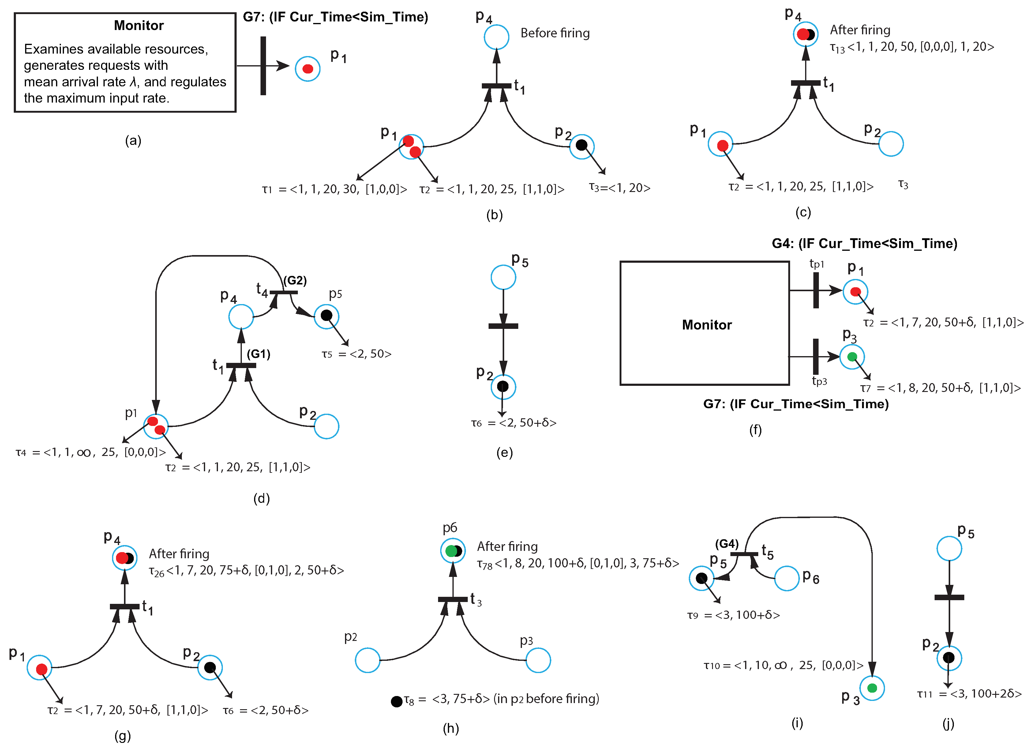
Let us assume an initial marking with two jobs (red tokens) in place p 1 and a token in place p 2 that is, there are two jobs that require the dominant resource and the system is ready to accept the next job request. These two jobs arrived at the same time. In Section 2, we mentioned the existence of m system queues. In each of these queues, there is a different dominant resource. Each user job entering a system queue, first makes a request for the dominant resource and then it proceeds to the next queues (if required) to request the non-dominant resources. The jobs are generated by a monitor entity, which examines the available resources and generates requests with mean arrival rate λ . Also, it can regulate the maximum arrival rate, using our probability based policy described in Section 2. The monitor operates for as long as the current time C u r _ T i m e is less than the total simulation time, which is defined by the user (see the guarding expression G7 of Figure 6a).
To describe how the simulator operates, let us consider an example, with these two jobs that have arrived to the system queue. Their requests are given in Table 2. The values of the black coupon τ 3 are: < 1 , 20 > .
At current time 20, there are two red tokens in place p 1 ( τ 1 , τ 2 ) and a black at p 2 ( τ 3 ) (see Figure 6b). We now use the ideas of Section 3.1.2 to determine the firing time of the only enabled transition t 1 . For the red tokens, the minimal stamp is 20 and because this value is found in both tokens, we choose the one with the smaller Job_Id = 1. Notice that the guard expression for t 1 is G1: (IF token_Id.ToRR = [1,x,x]), which is also true. Thus, t 1 can fire at time 20 + δ , where δ is a delay value. This value is produced by a random number generator with mean μ and it indicates the time required for the system to arrive to a new state according to the event that incurred by the transition’s firing. In our example, the service time is 30 time units. This means that the time elapsed until the token reaches p 4 should equal 30 and the newly generated token will be placed to p 4 at time = 50 time units. The result of this first firing are shown in Figure 6c: A red-black token is placed to p 4 and its values will be the union of the red and black tokens, that is: τ 12 = τ 1 τ 3 = < 1 , 1 , 20 , 30 + 20 , [ 0 , 0 , 0 ] , 1 , 20 > = < 1 , 1 , 20 , 30 + 20 , [ 0 , 0 , 0 ] , 1 , 20 > (see Section 3.1.1). Also, the resource request has been fulfilled, thus τ 13 . T o R R = [ 0 , 0 , 0 ] . Once t 1 fires, the fair allocation policy of Section 2 has completed its work, that is, it has determined a fair amount of DSQ resources for the job, the resources have been allocated and the next job to be processed can be determined. The token in p 4 activates t 4 at time 20 + 30 = 50 (notice the change at the red-black token of Figure 6c). Thus, the fair allocation policy procedure executes. However, the execution of t 4 will not produce an “actual token” to p 1 because the guard G2 is false. Instead, it will produce a red token with an time stamp. On the other side, the token produced for p 5 will be a black one. Figure 6d shows this situation. Now, a black token in p 5 activates t 2 and the processing of next request can start. Here, we consider the delay δ required to take the decision for the next job to be processed as a trivial latency, and we just write it as δ . Thus, the value of Arrival_Time for token τ 6 is 50 + δ as seen in Figure 6e. Now, transition t 1 is enabled: because the condition (see Section 3.2.3 for the description of the guard expressions used here):
G 1 : ( IF token _ Id . ToRR = [ 1 , x , x ] )   or   ( IF 2 . ToRR = [ 1 , x , x ] )
holds for the next chosen token with token_id = 2 (which also has a time stamp of 20 time units). By applying the firing time strategy of Section 3.1.2 we find that the process of resource allocation will start for τ 2 at time 50 + δ (the maximum of the two time stamps in positions p 1 and p 2 ).
For the second request, when the monitor sees the request [ 1 , 1 , 0 ] , it places one green token in p 3 as seen in Figure 6f using the transition t p 3 . Now, there are two transitions enabled, but because the condition
G 3 : ( IF token _ Id . ToRR = [ 0 , 1 , x ] )
does not hold, t 3 will not fire. However t 1 can fire and this will place a token in p 4 (see Figure 6g). Now, the newly generated red-black token proceeds as explained before for τ 1 , until it reaches p 2 , where it places a black token τ 8 = < 3 , 75 > . This will be used for the firing of t 3 next. Now, the DSQ request has been fulfilled and the execution of t 4 has updated the ToRRs for both the green and red tokens to [0,1,0]. Now, transition t 1 is not enabled because of G1, but now t 3 can fire since the condition
G 3 : ( IF token _ Id . ToRR = [ 0 , 1 , x ] )
now holds. Thus, the fair resource allocation policy can be implemented and a green-black token will be placed to p 6 (see Figure 6h). Then t 5 is enabled and, as before, a token with infinite time stamp will be placed to p 3 while p 5 will get a black token, which indicates the beginning of processing for the next request (see Figure 6i,j).
Now, if a third token appears with requests [1,1,1], the same form of execution will follow, but with some differences:
1.
The monitor will place a red, a green, and a blue token to p 1 , p 3 , and p 8 respectively, with initial ToRR = [1,1,1].
2.
Transition t 1 will have priority over t 3 and t 6 until the DSQ request is fulfilled. Then, a token with infinite time stamp will be placed to p 1 .
3.
Transition t 3 will have priority over t 6 until the Q 2 request is fulfilled. Then, a token with infinite time stamp will be placed to p 3 .
4.
Transition t 6 will have the lowset priority. When the Q 3 request is fulfilled, a token with infinite time stamp will be placed to p 8 .
Finally, if a job requires extra resources, it makes the request and the monitor treats it as a new token, so that it keeps a fair policy in the way the tasks take turns for requesting resources.

4.2. Experiments with CPNRA

For our simulation environment, we used an Intel Core i7-8559U Processor system, with clock speed at 2.7 GHz, equipped with four cores and eight threads/core, for a total of 32 logical processors. In our simulations, each user is entitled of up to 4 CPUs, 4 GB RAM and 40 GB of system disk. We also set that one CPU is one CPU unit, 1 GB RAM is one memory unit and 10 GB disk is one disk unit. Thus, the demand (2 CPUs, 1 GB RAM and 10 GB disk) is translated into (2,1,1) and it is CPU-intensive and the demand (1 CPU, 3 GB RAM, and 20 GB disk) is translated into (1,3,2) and it is memory-intensive. In our experimental results, we used our CPN based simulator to study the effect of the job input rate control and the system utilization. Finally, we studied the average response time, that is the average time between a transition activation and the actual firing (triggering) that causes a system change. This particular study will be supported by some more mathematical background, which we give in this section for clarity and convenience.

4.2.1. Job Input Rate Control

To study the effect of job generation rate, we worked as follows:
1.
We generated a random number of users, from 50–2000, and a set of requests for each user. We run two sets of simulations. In every experiment, we used different total amounts of each available resource (CPU, Memory, Disk), so that in some cases the resources available were enough to satisfy all user requests, while in other cases, they were not. For example, in one experiment, the total number of resources was (1 K, 1024, 10,000), that is (1024 CPUs, 1 Tb memory, 100 Tb disk) while for next this number could be double or half and so forth.
2.
We set the value of μ equal to 30 jobs per second, thus, the system’s input rate was at most λ = 30 jobs per second.
3.
We kept tracing the system’s state at regular time intervals h and recorded the percentage of resources consumed between consecutive time intervals, thus, we computed the b i values. Every time a job i leaves a queue, the system’s state changes. For example, if a job leaves the DSQ, it means that it has consumed F units of the dominant resource, changing the system’s state from K = K 1 , K 2 , K m to K = K 1 F , K 2 , K m . On the other hand, when multiple jobs enters a queue, the acceptable job input may be regulated accordingly, based on the model presented in Section 2.
After running sets of simulations for different user numbers (from 50 to 2000), we averaged the percentage of resources consumed during all the recorded time intervals, for different recorded values of λ i . The results are shown in Figure 7a,b. For Figure 7a, the total numbers of resources were (1 K, 1024, 10,000) and the number of users was between 50 and 1000, while for Figure 5b, the total number of resources were double (2K, 2048, 20,000) and the number of users was from 1000 to 2000. When the number of users was relatively small (50–200), an average value of input rate λ i = 15 was enough to exhaust almost 100% of the resources during the successive intervals. A larger number of users increases the competition for resources, thus the fair allocation policy is obliged to deliver far less resources than the requested to each job. As the job service time was considered to be constant, a larger input rate of λ i = 26.5 jobs/s (among all queues) was necessary to exhaust the resources requested over the time intervals when the number of users was 1000. This is more obvious in the second set of experiments, where we doubled the number of users and the available resources. Notice that in order to exhaust the resources, average input rates close to the maximum were required (see Figure 7b), from 28–30 jobs/s.

4.2.2. Resource Utilization

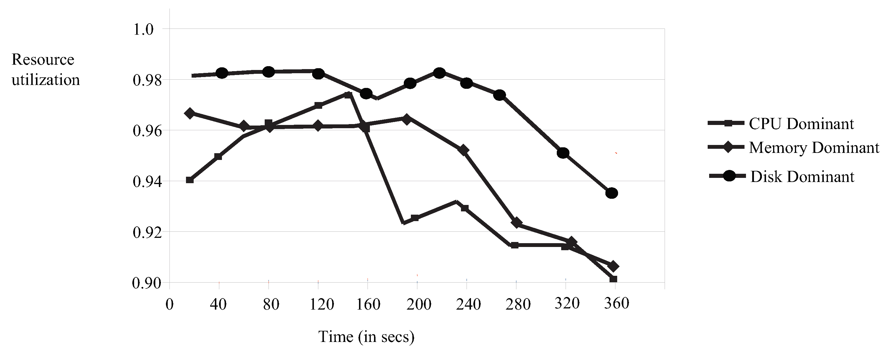
Next, we used our simulator to study the utilization of each resource independently. The requests were generated in such a manner, that the CPU was dominant for 40% of the cases, the memory was dominant for 30% of the cases and the disk was dominant in 30% of the cases and the number of users ranged between 50 and 1000. In all the simulation sets, the duration period was 360 s. As the time proceeded and resources were being consumed, fewer jobs were generated and the overall resource utilization decreased, but it never dropped below 90%. As can be seen in Figure 8, the CPU utilization begins dropping after about 160 s while the utilization of memory and disk seems to be dropping in a smoother way and at a later time (200 and 240 s, respectively). The peaks seen in this graph represent the cases where some more resources become available and return to the pool, either due to the allocation policy or due to returns from finished jobs that return the resources back to the pool.
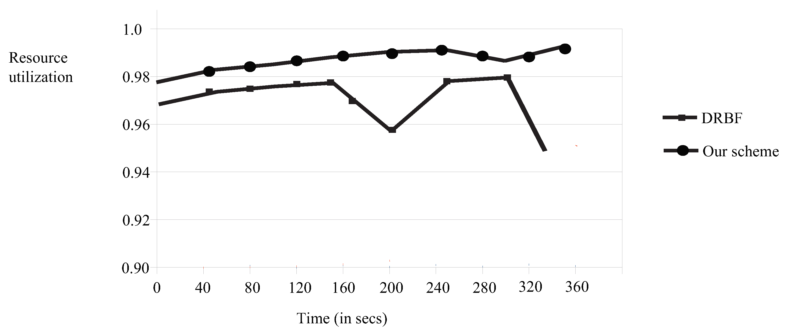
In our last set of experiments, we averaged the utilization of all the resources under our policy using a small number of users (up to 20), to fairly compare the utilization provided by our policy to the utilization provided by a new algorithm DRBF [33], where the authors reported their results for only a few users. The results are displayed in Figure 9. Again, our simulator verified that our resource allocation strategy outperforms the DRBF strategy and achieves utilization of about 98–99% while the changes are very small (notice that the line is rather smooth). The DRBF policy achieves a utilization of about 94–98%, with some peaks where the utilization drops off in a non-smooth fashion. Also, note that our strategy was found to achieve a utilization of over 90%, even for larger number of users, which is not proven for the DRBF scheme.

4.2.3. Average Response Time

In Reference [36], it has been proven that the mean number of jobs N ^ in a service center i is equal to the product of the mean arrival rate λ i by the average response time (also known as turnaround time), t ^ i . The average response time is the time a jobs spends inside the service center:
N ^ i = λ i t ^ i = p i 1 p i .
Now, the average response time is
t ^ i = N ^ i λ i = p i λ i ( 1 p i ) .
Now, using Equation (3), we replace λ i with p i × μ to get:
t ^ i = p i ( p i × μ ) ( 1 p i ) = 1 μ ( 1 p i ) .
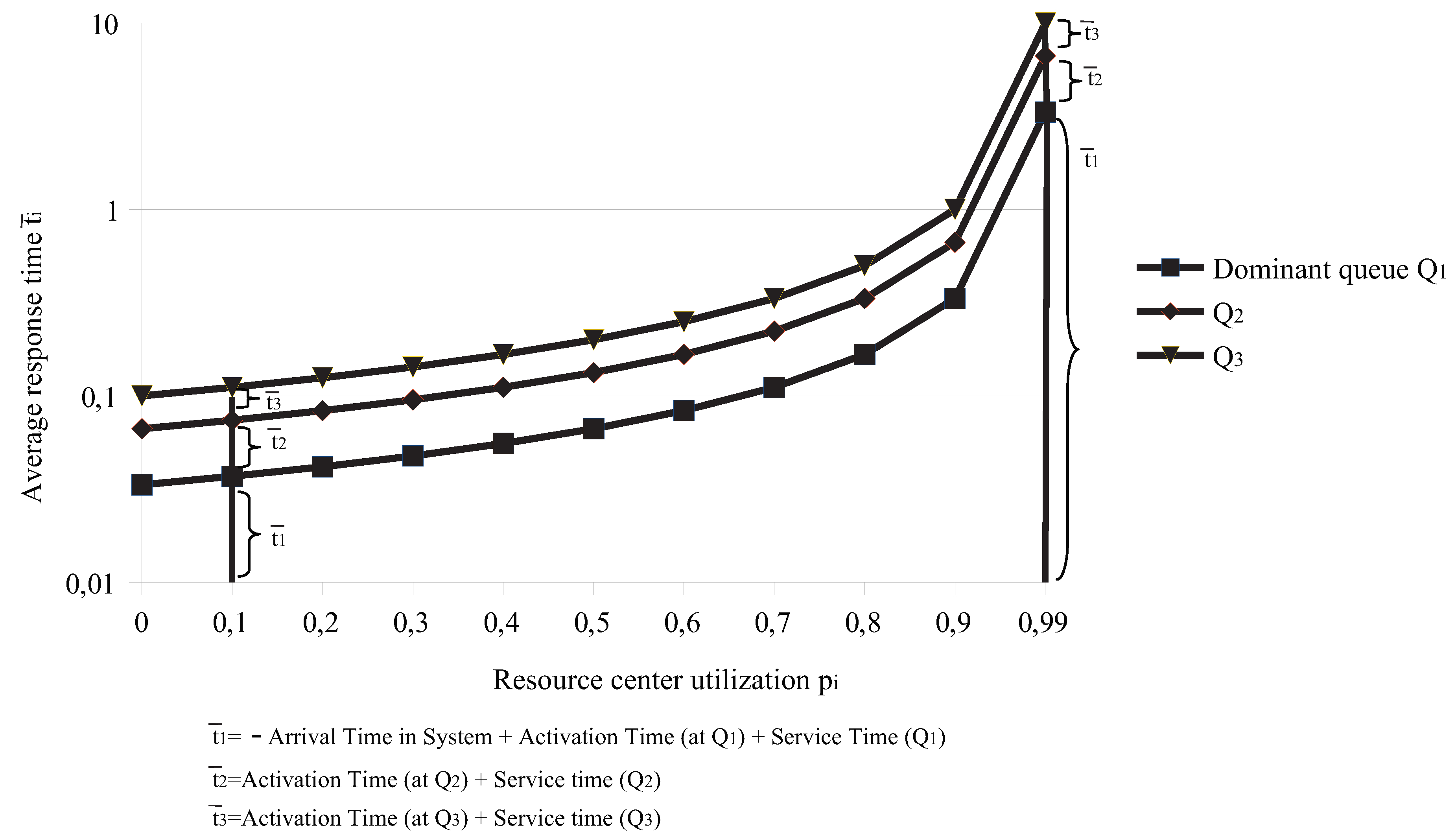
Since p i is the resource server utilization, Equation (10) states that as the resource utilization increases, the average response time also increases.
In Figure 10, we present some average total response times for a simulation that was executed for 3600 s (1 h) and a number of 300 users, which request all 3 resources. The reason we “forced” the user jobs to request all the resources available was to have “fair” comparisons for the average response times computed for different system utilization values. For example, if some jobs requested only the dominant resource, their average response time would be far less compared to the corresponding time for jobs that request all the resources. As in the other simulation sets, we set the value of μ for every queue equal to 30 jobs per second, thus, the system’s input rate was at most λ = 30 . Similar results can be obtained even if we use different μ values for the queues. In this set, we use a constant value of μ for simplicity. The total response time t ^ T o t a l is the sum of the response times computed per queue:
t ^ T o t a l = 1 μ i = 1 3 1 1 p i + Δ ,
where Δ is the time elapsed between the job arrival in the system and the sum of the times that it is ready to be served (that is, the corresponding transition is enabled) and the actual service time (transition firing and application of the relative changes in the system’s status). In Figure 10 we show these t ^ i values for system utilization 0.1 and for a system utilization that approaches 1. When the system utilization was 0.1, we had a mean arrival rate of λ = 3 jobs/s and the mean response time for all the user jobs (or tokens in the model) was found to be 0.04 s. When the system utilization approached 1, we had a mean arrival rate of λ 30 jobs/s and the mean response time for all the user jobs (or tokens in the model) was found to be 10 s. For a utilization equal to zero, from Equation (10) we can see that the minimum average response time for all the jobs approaches 0.03 s. Thus, when the system utilization is 0.1, then, the tokens remain in the system 0.04 / 0.03 = 1.33 times the minimum value of t ^ , while when the system utilization approaches 1, the tokens remain in the system about 10 / 0.03 = 333 times the minimum value of t ^ .

5. Conclusions and Future Work

In this paper, we extended our previous work [1], where we presented a fair resource allocation policy for cloud computing, which is includes a job generation (or flow) control, to determine the maximum number of affordable user tasks at a time period. Specifically, we produced a deadlock-free CPN model, which formed the basis for the development of our new CPNRA resource allocation simulator for clouds. The simulator is simple and its basic components are the cores, one for each queue system. Also, it presents no deadlocks and implements in a straightforward way our scheme. Another advantage is that it can easily be expanded for large number of resources, due to its hierarchical structure. Then, we used the simulator to analyze the system’s performance and we verified that the flow control can help to improve the resource utilization.
In the future, we plan to add more features to our simulator, so that it can be used to execute more different schemes. This will be a challenge, as many different resource allocator strategies can be found in the literature. This will help us with to produce comparable results for larger networks. Moreover, we need to improve the proposed allocation policy, so that it addresses other important issues like the cost of each resource allocated and the execution time. One idea we currently work on in order to reduce the total execution time is to pipeline the computations, but careful design is required to avoid delays between the pipeline [37] stages. Also, the introduction of a CPU/GPU combination would be of high interest, especially for large scale networks [38]. In this case, the model, and thus the simulator, has to be equiped with cores which are able to model the pipeline operations. Finally, we need to expand this simulator, so that, apart from resource allocation, it will include job scheduling strategies. This is specifically important, as the number of big data applications running over the cloud is getting larger and larger.

Author Contributions

Conceptualization, S.S., methodology, S.S.; software, S.S., S.K., and S.A.; validation, S.S. and S.K.; formal analysis, S.S., and S.A.; investigation, S.A., S.K., and S.A., resources, S.K., S.A., writing—original draft preparation, S.S., S.K., S.A.; writing—review and editing, S.S., S.K.; funding acquisition, S.A. All authors have read and agreed to the published version of the manuscript.

Funding

This research was funded by the University of Western Macedonia, Faculty of Education, Department of Early Childhood Education.

Conflicts of Interest

The authors declare no conflict of interest.

Abbreviations

The following abbreviations are used in this manuscript:
PNPetri Nets
CPNColored Petri Nets
CPNRAColored Petri Net-based Resource Allocation
ToRRType_of_Resources_Requested

References

  1. Souravlas, S.; Katsavounis, S. Scheduling Fair Resource Allocation Policies for Cloud Computing through Flow Control. Electronics 2019, 8, 1348. [Google Scholar] [CrossRef] [Green Version]
  2. Lu, Z.; Takashige, S.; Sugita, Y.; Morimura, T.; Kudo, Y. An analysis and comparison of cloud data center energy-efficient resource management technology. Int. J. Serv. Comput. 2014, 23, 32–51. [Google Scholar] [CrossRef]
  3. Jennings, B.; Stadler, R. Resource management in clouds: Survey and research challenges. J. Netw. Syst. Manag. 2015, 2, 567–619. [Google Scholar] [CrossRef]
  4. Tantalaki, N.; Souravlas, S.; Roumeliotis, M.; Katsavounis, S. Pipeline-Based Linear Scheduling of Big Data Streams in the Cloud. IEEE Access 2020, 8, 117182–117202. [Google Scholar] [CrossRef]
  5. Tantalaki, N.; Souravlas, S.; Roumeliotis, M.; Katsavounis, S. Linear Scheduling of Big Data Streams on Multiprocessor Sets in the Cloud. In Proceedings of the 2019 IEEE/WIC/ACM International Conference on Web Intelligence (WI), Thessaloniki, Greece, 14–17 October 2019; pp. 107–115. [Google Scholar]
  6. Alam, A.B.; Zulkernine, M.; Haque, A. A reliability-based resource allocation approach for cloud computing. In Proceedings of the 2017 7th IEEE International Symposium on Cloud and Service Computing, Kanazawa, Japan, 22–25 November 2017; pp. 249–252. [Google Scholar]
  7. Kumar, N.; Saxena, S. A preference-based resource allocation in cloud computing systems. In Proceedings of the 3rd International Conference on Recent Trends in Computing 2015 (ICRTC-2015), Delhi, India, 12–13 March 2015; pp. 104–111. [Google Scholar]
  8. Lin, W.; Wang, J.Z.; Liang, C.; Qi, D. A threshold-based dynamic resource allocation scheme for cloud computing. Procedia Eng. 2011, 23, 695–703. [Google Scholar] [CrossRef] [Green Version]
  9. Tran, T.T.; Padmanabhan, M.; Zhang, P.Y.; Li, H.; Down, D.G.; Beck, J.C. Multi-stage resource-aware scheduling for data centers with heterogeneous servers. J. Sched. 2015, 21, 251–267. [Google Scholar] [CrossRef]
  10. Hu, Y.; Wong, J.; Iszlai, G.; Litoiu, M. Resource provisioning for cloud computing. In Proceedings of the 2009 Conference of the Center for Advanced Studies on Collaborative Research, Toronto, ON, Canada, 2–5 November 2009; pp. 101–111. [Google Scholar]
  11. Khanna, A. RAS: A novel approach for dynamic resource allocation. In Proceedings of the 1st International Conference on Next Generation Computing Technologies (NGCT-2015), Dehradun, India, 4–5 September 2015; pp. 25–29. [Google Scholar]
  12. Saraswathia, A.T.; Kalaashrib, Y.R.A.; Padmavathi, S. Dynamic resource allocation scheme in cloud computing. Procedia Comput. Sci. 2015, 47, 30–36. [Google Scholar] [CrossRef] [Green Version]
  13. Xiao, Z.; Song, W.; Chen, Q. Dynamic resource allocation using virtual machines for cloud computing environment. IEEE Trans. Parallel Distrib. Syst. 2013, 24, 1107–1117. [Google Scholar] [CrossRef]
  14. Mansouri, N.; Ghafari, R.; Zade, B.M.H. Mohammad Hasani Zade: Cloud computing simulators: A comprehensive review. Simul. Model. Pract. Theory 2020. [Google Scholar] [CrossRef]
  15. Calheiros, R.N.; Ranjan, R.; Beloglazov, A.; De Rose, C.A.; Buyya, R. CloudSim: A toolkit for modeling and simulation of cloud computing environments and evaluation of resource provisioning algorithm. Softw. Pract. Exp. 2011, 41, 23–50. [Google Scholar] [CrossRef]
  16. Garg, S.K.; Buyya, R. Networkcloudsim: Modelling parallel applications in cloud simulations. In Proceedings of the 4th IEEE International Conference on Utility and Cloud Computing, Victoria, NSW, Australia, 5–8 December 2011; pp. 105–113. [Google Scholar]
  17. Wickremasinghe, B.; Calheiros, R.N.; Buyya, R. CloudAnalyst: A CloudSim-based visual modeller for analysing cloud computing environments and applications. In Proceedings of the 24th IEEE International Conference on Advanced Information Networking, Perth, WA, Australia, 20–23 April 2010; pp. 446–452. [Google Scholar]
  18. Calheiros, R.N.; Netto, M.A.; De Rose, C.A.; Buyya, R. EMUSIM: An integrated emulation and simulation environment for modeling, evaluation, and validation of performance of cloud computing applications. Softw. Pract. Exp. 2013, 43, 595–612. [Google Scholar] [CrossRef]
  19. Fittkau, F.; Frey, S.; Hasselbring, W. CDOSim: Simulating cloud deployment options for software migration support. In Proceedings of the IEEE 6th International Workshop on the Maintenance and Evolution of Service-Oriented and Cloud-Based Systems, Trnto, Italy, 24 September 2012; pp. 37–46. [Google Scholar]
  20. Li, X.; Jiang, X.; Huang, P.; Ye, K. DartCSim: An enhanced user-friendly cloud simulation system based on CloudSim with better performance. In Proceedings of the IEEE 2nd International Conference on Cloud Computing and Intelligence Systems, Hangzhou, China, 30 October–1 November 2012; pp. 392–396. [Google Scholar]
  21. Sqalli, M.H.; Al-Saeedi, M.; Binbeshr, F.; Siddiqui, M. UCloud: A simulated Hybrid Cloud for a university environment. In Proceedings of the IEEE 1st International Conference on Cloud Networking, Paris, France, 28–30 November 2012; pp. 170–172. [Google Scholar]
  22. Kecskemeti, G. DISSECT-CF: A simulator to foster energy-aware scheduling in infrastructure clouds. Simul. Model. Pract. Theory 2015, 58, 188–218. [Google Scholar] [CrossRef] [Green Version]
  23. Tian, W.; Zhao, Y.; Xu, M.; Zhong, Y.; Sun, X. A toolkit for modeling and simulation of real-time virtual machine allocation in a cloud data center. IEEE Trans. Autom. Sci. Eng. 2015, 12, 153–161. [Google Scholar] [CrossRef]
  24. Fernández-Cerero, D.; Fernández-Montes, A.; Jakobik, A.; Kołodziej, J.; Toro, M. FSCORE: Simulator for cloud optimization of resources and energy consumption. Simul. Model. Pract. Theory 2018, 82, 160–173. [Google Scholar] [CrossRef]
  25. Gupta, S.K.; Gilbert, R.R.; Banerjee, A.; Abbasi, Z.; Mukherjee, T.; Varsamopoulos, G. GDCSim: A tool for analyzing green data center design and resource management techniques. In Proceedings of the International Green Computing Conference and Workshops, Orlando, FL, USA, 25–28 July 2011; pp. 1–8. [Google Scholar]
  26. Kristensen, L.M.; Jørgensen, J.B.; Jensen, K. Application of Coloured Petri Nets in System Development. In Lecture Notes in Computer Science; Springer: Berlin/Heidelberg, Germany, 2003; pp. 626–685. [Google Scholar]
  27. Peterson, J.L. Petri nets. ACM Surv. 1997, 9, 223–252. [Google Scholar] [CrossRef]
  28. Souravlas, S.I.; Roumeliotis, M. Petri Net Based Modeling and Simulation of Pipelined Block-Cyclic Broadcasts. In Proceedings of the 15th IASTED International Conference on Applied Simulation and Modelling-ASM, Rhodos, Greece, 26–28 June 2006; pp. 157–162. [Google Scholar]
  29. Shojafar, M.; Pooranian, Z.; Abawajy, J.H.; Meybodi, M.R. Abawajy, and Mohammad Reza Meybodi: An Efficient Scheduling Method for Grid Systems Based on a Hierarchical Stochastic Petri Net. J. Comput. Sci. Eng. 2013, 7, 44–52. [Google Scholar] [CrossRef] [Green Version]
  30. Shojafar, M.; Pooranian, Z.; Meybodi, M.R.; Singhal, M. ALATO: An Efficient Intelligent Algorithm for Time Optimization in an Economic Grid Based on Adaptive Stochastic Petri Net. J. Intell. Manuf. 2013, 26, 641–658. [Google Scholar] [CrossRef]
  31. Barzegar, S.; Davoudpour, M.; Meybodi, M.R.; Sadeghian, A.; Tirandazian, M. Traffic Signal Control with Adaptive Fuzzy Coloured Petri Net Based on Learning Automata. In Proceedings of the 2010 Annual Meeting of the North American Fuzzy Information Processing Society, Toronto, ON, Canada, 12–14 July 2010; pp. 1–8. [Google Scholar]
  32. Ghodsi, A.; Zaharia, M.; Hindman, B.; Konwinski, A.; Shenker, S.; Stoica, I. Dominant resource fairness: Fair allocation of multiple resource types. NSDI 2011, 11, 323–336. [Google Scholar]
  33. Zhao, L.; Du, M.; Chen, L. A new multi-resource allocation mechanism: A tradeoff between fairness and efficiency in cloud computing. China Commun. 2018, 24, 57–77. [Google Scholar] [CrossRef]
  34. Souravlas, S. ProMo: A Probabilistic Model for Dynamic Load-Balanced Scheduling of Data Flows in Cloud Systems. Electronics 2019, 8, 990. [Google Scholar] [CrossRef] [Green Version]
  35. Souravlas, S.I.; Roumeliotis, M. Petri net modeling and simulation of pipelined redistributions for a deadlock-free system. Cogent Eng. 2015, 2, 1057427. [Google Scholar] [CrossRef]
  36. Little, J.D.C. A Proof for the Queuing Formula L = λW. Oper. Res. 1961, 9, 383–387. [Google Scholar] [CrossRef]
  37. Souravlas, S.; Roumeliotis, M. A pipeline technique for dynamic data transfer on a multiprocessor grid. Int. J. Parallel Programm. 2004, 32, 361–388. [Google Scholar] [CrossRef]
  38. Souravlas, S.; Sifaleras, A.; Katsavounis, S. Hybrid CPU-GPU Community Detection in Weighted Networks. IEEE Access 2020, 8, 57527–57551. [Google Scholar] [CrossRef]
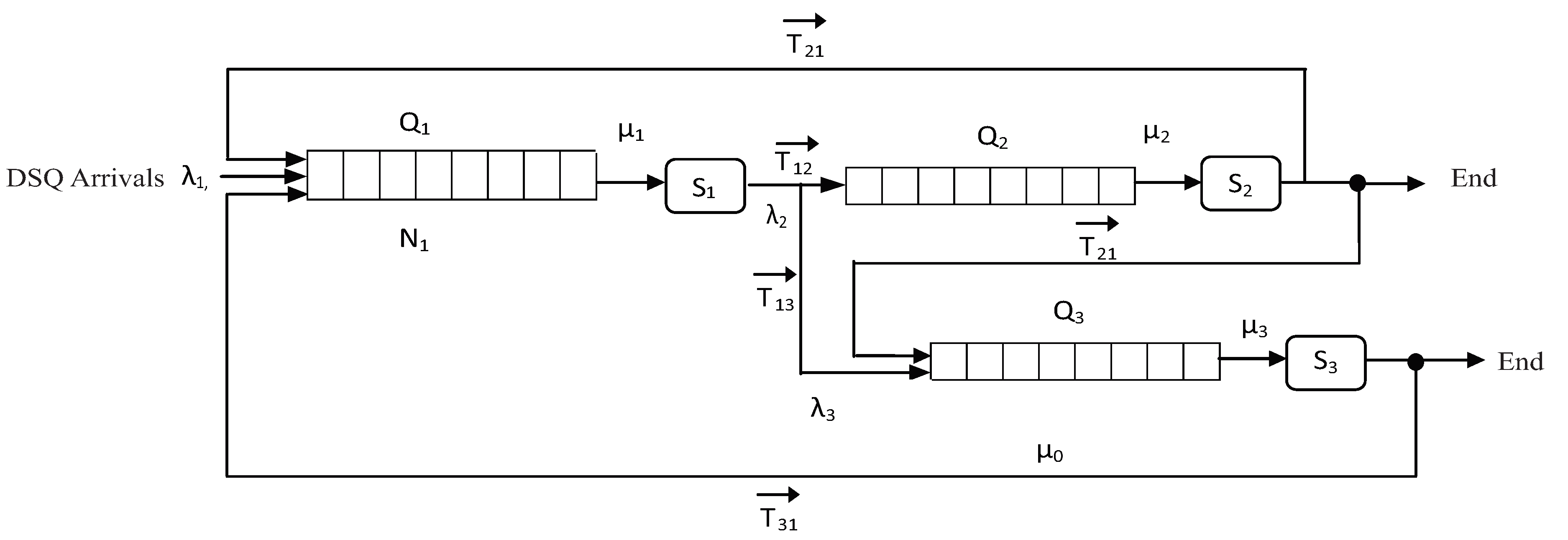
Figure 1. Resource allocation model with 3 resources, i = 1 is the dominant resource.
Applsci 10 05644 g001
Figure 2. Resource Allocator with m Queue Systems.
Applsci 10 05644 g002
Figure 3. Example of an Enabled Transition in a Colored Petri Nets (CPN).
Applsci 10 05644 g003
Figure 4. The dominant server queue (DSQ) core.
Applsci 10 05644 g004
Figure 5. Transition firing time example.
Applsci 10 05644 g005
Figure 6. Simulation execution example.
Applsci 10 05644 g006
Figure 7. The DSQ core.
Applsci 10 05644 g007
Figure 8. Individual resource utilization over a period of one hour.
Applsci 10 05644 g008
Figure 9. Average resource utilization with small number of users (up to 20).
Applsci 10 05644 g009
Figure 10. Average response times.
Applsci 10 05644 g010
Table 1. Summary of related papers, based on the metrics used to evaluate resource allocation.
Paper ReferenceCostExecution TimeUtilization
[6]YesNoNo
[7]YesNoYes
[8]YesYesNo
[10]YesNoNo
[11]NoNoYes
[9]YesYesNo
[12]NoYesYes
[13]NoYesYes
Our workNoNoYes
Table 2. An execution example.
Job_IdPriorityArrival_ TimeService_TimeType_of_Resources_Requested
112030[1,0,0]
212025[1,1,0]