A Tutorial for Feature Engineering in the Prognostics and Health Management of Gears and Bearings

Abstract

Gears and bearings are one of the major components of many machines, which can result in operation downtime or even catastrophic failure of a whole system. This paper addresses a tutorial for the features extraction and selection of the gears and bearings, which is known as feature engineering, a prerequisite step for the prognostics and health management (PHM) of these components. While there have been many new developments in this field, no studies have addressed the tutorial aspects of features engineering to aid engineers in solving problems by their own effort, which is of practical importance for successful PHM. The paper aims at helping beginners learn the basic concepts, and implement the algorithms using the public datasets as well as those made by the authors. Matlab codes are provided for them to implement the process by their own hands.

1. Introduction

Prognostics and health management (PHM) is an engineering discipline that identifies fault severity and predicts the remaining useful life (RUL) of the target system. PHM is the enabling technology towards condition-based maintenance (CBM), which is the future maintenance strategy as opposed to corrective maintenance (CM) and periodic maintenance (PM). Numerous books have been published recently addressing various aspects such as signal processing [1], data driven diagnostics [2,3], prognostics [4], and practical applications [5,6]. In general, PHM consists of three steps: (1) data acquisition and features extraction, (2) fault diagnosis, and (3) failure prognosis [7,8,9]. As PHM is performed from signals that are obtained from sensors such as vibration, acoustic emissions, or oil debris, it is crucial to remove undesired noise and extract the valuable information called features from the raw signals in the first step. Based on the extracted features, the fault mode and its severity are identified through the diagnosis, and RUL is predicted using the prognosis algorithm. While there are many useful features for this purpose today, good features vary depending on PHM steps and applications. For example, in the diagnosis, features should show a clear difference between the normal and fault states to distinguish the health condition. In the prognosis, on the other hand, features showing a monotonic trend over time are considered good indicators for RUL prediction. In this context, the process to obtain such good features is also called “feature engineering”.

In rotating machinery, gears and bearings are important components because they transmit power while supporting the applied load in the system. Therefore, their unexpected failure and degradation during operation lead to economic loss and catastrophic accidents. In fact, the failure of these components accounts for a large proportion of whole system failures [10], which is the reason why many are focusing on bearing and gear PHM. In this context, the feature engineering of these components is of crucial importance as well. While there have been many studies in this area, their concern was mostly on new algorithm development including the deep learning approaches recently gaining popularity [11,12]. Relatively less attention was given to the educational aspects for beginners to implement this work by themselves. Motivated by this lack of attention, this paper presents a tutorial for feature engineering for gears and bearings.

Recently, authors have published a series of tutorial papers for other subjects with the same objective: Aid engineers to gain better understanding of PHM and implement it by the codes. The first was Particle Filter algorithm with the example of battery degradation and crack growth problems to demonstrate the model-based prognosis, which is the last step of PHM [4]. Second was advanced signal processing using public datasets of gears and bearings, which is the very first step of PHM [13]. This paper is another tutorial effort, as a continuation from the signal processing. As in the previous tutorial, public datasets released from other institutions are used as well as those made by the authors. Matlab codes are provided in Appendix A for engineers to implement the feature engineering process by their own hands.

2. PHM Framework and Datasets for the Tutorial

The PHM framework can be divided into several steps as shown in Figure 1. After the data acquisition, the signal processing step is performed which aims to remove noise from the raw signal to obtain only the necessary information for the diagnosis and prognosis. Discrete signal separation techniques remove the periodic signals that are not related to the fault such as the ones transmitted from nearby equipment. Residual fault signals are then enhanced by signal enhancement techniques. If necessary, the signals, whether in their raw form or after processing, can also be decomposed into various components to facilitate the exploration of fault information. Detailed information about the techniques is addressed in the previous tutorial study [13]. Once the signal processing is done, the feature engineering process is conducted next, where the features that represent the fault or degradation of the system can be extracted, evaluated, and selected as shown in Figure 1. Finally, by exploiting these features, fault diagnosis is performed to classify the state of the target system or failure prognosis is performed to predict when the failure will occur in the future.

Note that feature engineering requires substantial skills and expertise, which is the key to the success of the subsequent steps: diagnosis and prognosis. Recently, there is a new trend that takes advantage of deep learning-based neural network approaches to avoid the feature engineering process as illustrated in Figure 2 [11]. The deep learning-based method utilizes the raw data directly in the diagnosis right after the signal processing, as opposed to the traditional data-driven method that underlies the feature engineering process. However, since the deep learning–based method is not mature yet and poses several challenges to be addressed in the future, this tutorial presents the traditional feature engineering method, aided by Matlab implementations.

In the PHM study of gears and bearings, the general method of data acquisition is to measure vibration by attaching an accelerometer to the housing of gears or bearings. Gathering the data is, however, too expensive, requiring a test rig, sensors, and time-consuming tests. To avoid this, several universities and research institutions have released their data to the public, which are summarized in reference [13]. They are classified into diagnostic and prognostic data. Diagnostic data are obtained by running the components under normal and fault conditions, respectively. Prognostic data are obtained by running the components constantly from the normal to the failure state. Among them, the data used in this paper are presented in

Table 1. Dataset explanation.

Name of Dataset	Data Type	Sensor Type	Number of Dataset
HS (Gear) [14]	Diagnosis	Acceleration	Normal		Fault
			6		11
KAUG (Gear)	Diagnosis	Encoder	Normal	Spall		Crack
			10	10		11
CWRU (Bearing) [15]	Diagnosis	Acceleration	Normal	Inner		Outer
			10	10		10
IMS (Bearing) [16]	Prognosis	Acceleration	3

and the details are as follows: HS (High speed) gear dataset [14] is the vibration data obtained for 6 s with a sampling frequency of 97,656 Hz from the 3 blades upwind V90 wind generator, which produces an output of 3 MW and operates at 30 Hz. The gear has 32 teeth and the gear mesh frequency (GMF) is 960 Hz. The data are collected in the normal and fault conditions, in which the natural faults are applied in the pinion gear. Among 17 files, 11 are fault and 6 are normal. The next dataset is KAUG (Korea Aerospace University Gear), obtained from the gearbox testbed made by the authors. The encoder signals are acquired from the testbed at a 10 kHz sampling rate. There are 31 data files, of which 10 are normal, 10 spall, and 11 crack. The KAUG datasets are given on the authors’ homepage www.kau-sdol.com. The CWRU bearing dataset is provided by Case Western Reverse University [15]. Two bearings are installed at the motor drive- and fan- end, which are operated under various motor loads and speeds. Among the many cases, this study considers the fault data at the inner and outer race of the drive-end with the hole diameter of 0.021 inches. The operating load is 3 HP, speed is 1730 rpm, and sampling frequency is 12 kHz. In the case of CWRU, a single dataset in each fault is divided into 10 segments to create 10 sets of data for the diagnostic study. The last dataset is the run-to-fail data for the prognostic study provided by the Center for Intelligent Maintenance Systems (IMS) at University of Cincinnati [16]. The IMS bearing dataset has been collected from 4 bearings operating at 2000 rpm under 6000 lbs radial load applied to the shaft and bearing, with a sampling rate of 20,480 Hz. There are three datasets provided by the compressed file format. Each dataset has the damage announcement at the end of the experiment: Dataset 1 with inner race fault at bearing #3 and rolling element fault at bearing #4, dataset 2 with outer race fault at bearing #1, and dataset 3 with outer race fault at bearing #3.

3. Feature Extraction

Feature engineering begins with feature extraction from data in its raw form or after going through noise removal by signal processing. According to Caesarendra et al. [17], the features are usually divided into three categories: time domain, frequency domain, and time-frequency domain. Among these, time-domain features are the simplest and most widely used, and are not just limited to gears and bearings. On the other hand, there are some unique features specially developed for gears and bearings, respectively. These are addressed in the following sections.

3.1. Features for Gears

In feature engineering for gears, several signal processing steps are usually taken and appropriate features are extracted from each step that enable fault identification from the normal. This is explained in Figure 3, which indicates that the raw data are processed step by step, and after each step, relevant features are extracted. The signal in the time domain and its Fourier transform in the frequency domain are also illustrated. Note that the features are divided into two groups: general features, which are the time domain features shown by the blue dotted box, and specific features for the gears as shown by the red dotted box. Note that the latter have been developed specifically for gears, for improved capability of fault diagnosis as found in many articles in the literature (e.g., [18,19,20,21]).

As shown in Figure 3, the raw signal includes the shaft and GMF frequencies (and their harmonics) as well as the noise existing at the low frequencies in the frequency spectrum. The first step is to remove these unnecessary signals, by the time synchronous averaging (TSA) and high pass filtering (HPF). TSA is to average out the signal over each revolution to remove random noise occurring during the rotation, which can be executed by the Matlab built-in function x = tsa(x, fs, tach, ′PulsePerRotation′, ppr), where fs is the sampling frequency, tach is the tachometer signal, and ppr is PulsePerRotation. HPF is done to remove the low frequency components including the shaft and its harmonic frequencies, which are irrelevant to the gear fault. HPF first determines the filter parameters which are executed by the Matlab built-in function [b,a] = butter(ord, Wn, ′high′), where ord is the filter order, and Wn = sf/(fs/2) is the Nyquist frequency, which is the shaft frequency sf divided by fs/2. The filtering is then performed by x = filter(b, a, x). In this study, the filter order is given by 1. As the order increases, the filtering becomes sharp, which improves the passing performance, but decreases group delay characteristics, causing phase distortion. Hence, the filter order should be properly selected. In this paper, filter order is given by 1 among the values 1 to 3 often used in the filtering.

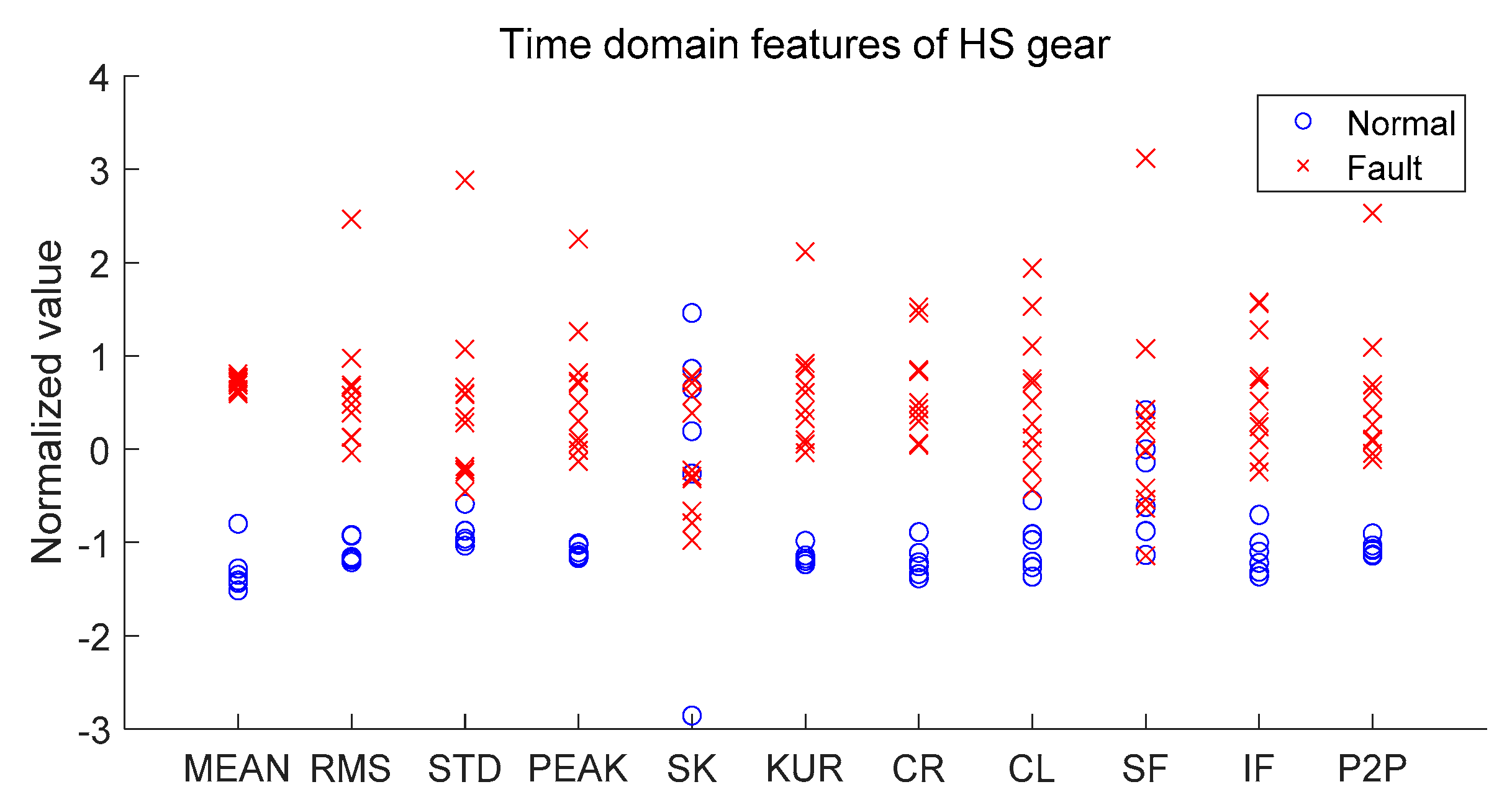
After this step, 11 time domain features are extracted, which are explained in

Table 2. General time domain features [17,22].

Abbreviation	Full Name	Brief Explanation	Formula	Matlab Functions
MEAN	Mean	Average	$\frac{\sum X}{N}$	mean(x)
RMS	Root mean square	Value that generally tends to get bigger as the degree of fault in the bearing increases	$\sqrt{\frac{\sum X^2}{N}}$	rms(x)
STD	Standard deviation	Value representing the dispersion of a signal	$\sqrt{\frac{\sum {\left(X-\overline{X}\right)}^2}{N-1}}$	std(x)
PEAK	Peak	Maximum value of signal absolute value	$\max \left(\left|X\right|\right)$	max(abs(x))
SK	Skewness	The asymmetry of the probability density function of the vibration signal	$\frac{\frac{1}{N}\sum {\left(X-\overline{X}\right)}^3}{ST{D}^3}$	skewness(x)
KUR	Kurtosis	The sharpness of the probability distribution of the vibration signal, and if this value is close to 3, it is closer to normal distribution	$\frac{\frac{1}{N}\sum {\left(X-\overline{X}\right)}^4}{ST{D}^4}$	kurtosis(x)
CF	Cres factor	The ratio of peak values to the RMS of a signal	$\frac{PEAK}{RMS}$	-
CL	Clearance factor	Peak value divided by the square of root mean	$\frac{\max \left(\left|X\right|\right)}{{\left(\frac{\sum \sqrt{X}}{N}\right)}^2}$	-
SF	Shape factor	RMS divided by mean	$\frac{RMS}{MEAN}$	-
IF	Impulse factor	The ratio of peak values to the mean of a signal	$\frac{PEAK}{MEAN}$	-
P2P	Peak to peak	The difference between maximum and minimum values of the signal	$\max \left(X\right)-\min \left(X\right)$	-

. Recall that the time domain features can be extracted either from the raw signal directly or after taking this step depending on the problem. The Matlab function to extract the time domain features is given in Appendix A as [feature, feature_name] = TimeFeatures(x), where feature and feature_name are the array of feature values and their names, respectively.

Figure 4 is the result of extracted time domain features for the example of HS gear dataset: 6 normal and 11 fault data, in which the acronyms are found in Table 2. Note that each set of feature data is normalized by mean and standard deviation, respectively. In the result, most of the features classify the fault (x) from the normal (o) well, but some (SK and SF) do not, which means that further processing is necessary to select only the useful features.

At this step, the gear specific features are extracted as shown in Figure 3, which are the figure of merits zero (FM0) and sideband energy ratio (SER). FM0 serves to detect changes in gear engagement patterns as an indicator of the gear’s main fault:

$$FM0=\frac{P{P}_x}{{\sum }_{i=1}^{N_{har}}{P}_i}.$$

(1)

where PP_x is the difference between the maximum and minimum of the time domain signal, P_i is the amplitude of the ith harmonic frequencies of GMF, and N_har is the number of harmonic frequencies. The GMF is the frequency caused by the engagement of gear teeth, given by the product of shaft frequency and number of teeth. In the frequency domain of gear signal, sidebands occur at both sides of the GMF and its harmonics with the interval of shaft frequency. SER is the ratio of the sum of sideband frequency amplitudes to that of the first harmonic of GMF:

$$SER=\frac{{\sum }_{i=1}^{N_{sb}}\left(S_i^{+}+S_i^{-}\right)}{P_1},$$

(2)

where P₁ is the amplitude at the first harmonic of GMF, N_sb is the number of sidebands, which is usually 3 [23], and $S_i^{+}$ and $S_i^{-}$ denote the amplitudes of the ith sideband at the first harmonic of GMF.

The next step is to obtain the residual signal by removing the components of GMF and their harmonics, which are those not related with the fault. From the residual signal, the feature NA4 is obtained, which is to detect progress of defects in gears. NA4 is obtained by dividing the fourth statistical moment of the residual signal ($res$) by the averaged variance of the residual signal over the last M revolutions, raised to the second power:

$$NA4=\frac{\frac{1}{N}{\sum }_{i=1}^N{\left(re{s}_i-\overline{res}\right)}^4}{{\left\{\frac{1}{M}{\sum }_{j=1}^M\left[\frac{1}{N}{\sum }_{k=1}^N{\left(re{s}_{jk}-\overline{re{s}_j}\right)}^2\right]\right\}}^2},$$

(3)

where N is the number of data points in one revolution, and $\overline{res}$ is the mean of $res$. NB4 is similar to NA4 except that instead of the residual signal, NB4 uses the envelope of band-pass filtered (BPF) signal centered at the GMF. The BPF is to leave the signals in the band while removing those outside. The feature was devised from the idea that a few damaged gear teeth will cause transient load fluctuations different from the normal fluctuations, which can be identified by the envelope (s) of BPF signal. NB4 is given by

$$NB4=\frac{\frac{1}{N}{\sum }_{i=1}^N{\left(s_i-\overline{s}\right)}^4}{{\left\{\frac{1}{M}{\sum }_{j=1}^M\left[\frac{1}{N}{\sum }_{k=1}^N{\left(s_{jk}-\overline{s_j}\right)}^2\right]\right\}}^2}.$$

(4)

Regarding the envelope, more detail is given in the next section for the bearing features extraction.

The third step is to obtain the difference signal by further removing the sideband frequencies of the GMF from the residual signal. From the difference signal, FM4, M6A, M8A, and energy ratio (ER) are extracted. FM4 is the feature to detect the pattern changes resulting from the damage on a few gear teeth. FM4 is defined as the kurtosis of the difference signal ($diff$):

$$FM4=\frac{N{\sum }_{i=1}^N{\left(dif{f}_i-\overline{diff}\right)}^4 }{{\left({\sum }_{i=1}^N{\left(dif{f}_i-\overline{diff}\right)}^2\right)}^2}.$$

(5)

This indicates that if $diff$ is from the normal gear, it will follow Gaussian noise so that the FM4 should be 3, whereas it will be greater than 3 if defective. M6A and M8A were developed to detect surface damage on machinery components. They are similar to FM4 except that M6A and M8A are more sensitive to peaks of the $diff$ signal with higher power with 6 and 8, respectively:

$$M6A=\frac{N^2{\sum }_{i=1}^N{\left(dif{f}_i-\overline{diff}\right)}^6}{{\left({\sum }_{i=1}^N{\left(dif{f}_i-\overline{diff}\right)}^2\right)}^3},$$

(6)

$$M8A=\frac{N^3{\sum }_{i=1}^N{\left(dif{f}_i-\overline{diff}\right)}^8}{{\left({\sum }_{i=1}^N{\left(dif{f}_i-\overline{diff}\right)}^2\right)}^4}.$$

(7)

ER was proposed to define the RMS of $diff$ signal divided by the amplitudes of the GMF and its harmonics with further addition by their respective sidebands:

$$ER=\frac{RMS\left(diff\right)}{{\sum }_{i=1}^{N_{har}}\left\{P_i+{\sum }_{j=1}^{N_{sb}}\left(S_{ij}^{+}+S_{ij}^{-}\right)\right\}}.$$

(8)

The Matlab functions to obtain the residual and difference signal are given by res_sig = res_gear(x,fs,gmf, cutoff,ord), and diff_sig = diff_gear (x,fs,gmf,sf,cutoff,ord), respectively. In the functions, cutoff is the bandwidth to filter out, and ord is the filter order. Within each function, the removal of the frequency component for the bandwidth [f₀-cutoff, f₀+cutoff] is carried out by the Matlab built-in function (b,a) = butter(ord,[f₀-cutoff f₀+cutoff],′stop′), followed by x = filter(b, a, x). This is also called notch filtering. Note that the cutoff is imposed to account for the inaccurate GMF, which usually occurs in practice. In the HS gear dataset, gmf = 960 Hz, cutoff = 2, ord = 1 are used. The Matlab function to extract all the above-mentioned gear specific features is given by [feature, feature_name] = Gear_feat(tsa_sig, res_sig, diff_sig, gmf, sf, fs). Figure 5 represents the result of extracted features for the HS gear. As in Figure 4, some are good classifiers, while others such as SER and M6A are not. Methods to select useful classifiers will be explained in Section 4.

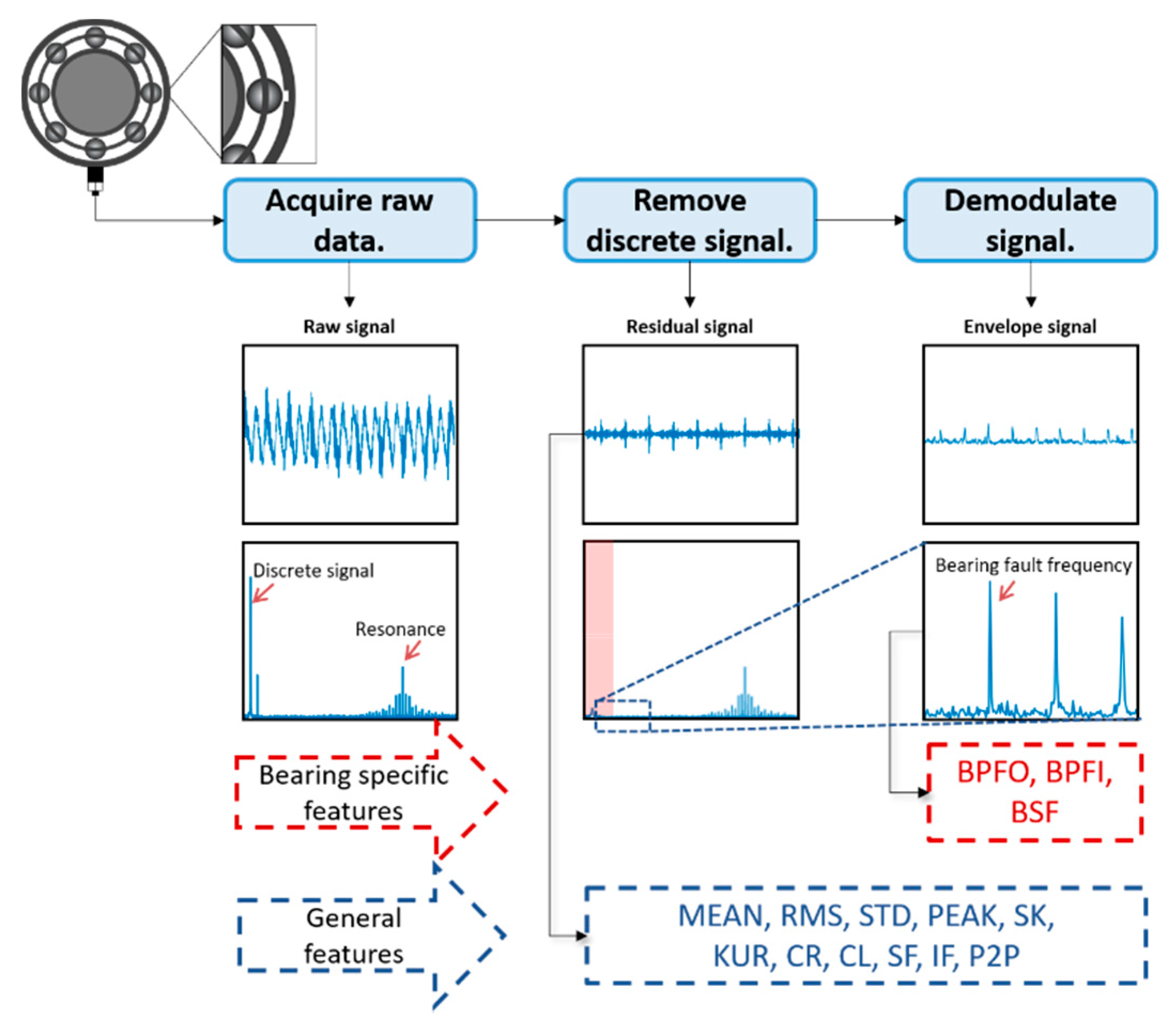
3.2. Features for Bearings

Figure 6 illustrates the typical features extraction process in the bearings PHM, of which the basic philosophy is the same: carry out the signal processing steps to remove unnecessary signal or noise. In general, the bearing signal consists of the discrete (predictable) part, which is irrelevant to the fault since it is from the other components such as the shaft or gears, and the remaining (unpredictable) part. With this in mind, the first step is to remove the discrete signal by using the autoregressive (AR) filter, which is to obtain the discrete part of the signal based on the past data for a certain period. Then the residual part of the signal, which may include the fault information, is obtained by subtracting this from the raw data. In the figure, this usually corresponds to the removal of the low frequency components in the frequency domain. The discrete signal is made by the AR model:

$$x_p\left(n\right)=-{\displaystyle \sum }_{k=1}^{p}a\left(k\right)x\left(n-k\right).$$

(9)

where x is the raw signal, x_p is the discrete (predicted) signal, n and k are the indices in time, a(k) and p are the parameters and order of the AR model, respectively. The residual signal is then obtained by

$$e\left(n\right)=x\left(n\right)-x_p\left(n\right).$$

(10)

The AR model is obtained by Matlab built-in functions a = aryule(x,p) followed by xp = filter([0 -a(2:end)],1,x). Note here that the order p should be assigned carefully since it affects the performance greatly: too high may include even the fault signal, too low may lose the periodicity in the prediction. In general, the order p is determined such that the kurtosis of the residual signal is maximized. General time domain features are extracted from the residual signal as depicted by the blue dotted box.

After removing the discrete signal with the AR filter, the next step is the demodulation of the signal. Whenever the fault exists in the race or elements, the bearing produces impact (fault) signals with a certain period called bearing fault frequencies. However, it is usually amplitude-modulated by much higher resonant frequencies, as found in Figure 6, which means that the fault signal is buried by the resonance signals. In order to separate the fault signal from this, envelope analysis, also called the demodulation process [13], is carried out to extract the amplitudes modulated by the carrier (resonance) signal. To this end a Hilbert transform is conducted, to shift the phase by −90 degrees. Then the so-called analytic signal is defined by extending the real signal to the imaginary dimension as follows:

$$x_{analytic}\left(t\right)=x\left(t\right)+j\widehat{x}\left(t\right),$$

(11)

where $\widehat{x}\left(t\right)$ is the Hilbert transformed signal. The envelope signal is then obtained by calculating the magnitude $x_{analytic}\left(t\right)$ by using the Matlab built-in function x = abs(Hilbert(x)). As a result, the signals of resonant (higher) frequencies are removed in the envelope signal, and only those of the bearing fault (lower) frequencies remain in the frequency domain as shown in the figure, from which the bearing-specific features can be extracted.

The bearing fault frequencies can be identified by the bearing geometry as shown in Figure 7. Bearings consists of inner, outer race and balls or rollers. If one of them includes the defect, the bearing produces signals at the specific frequencies while it rotates and passes through the defect. They are the ball pass frequency of outer race (BPFO), ball pass frequency of inner race (BPFI) and ball spin frequency (BSF), which are defined as follows [24]:

$$f_{BPFO}=w\frac{N_B}{D}\left(1-\frac{B_D}{D}\cos \left(\alpha \right)\right),$$

(12)

$$f_{BPFI}=w\frac{N_B}{D}\left(1+\frac{B_D}{D}\cos \left(\alpha \right)\right),$$

(13)

$$f_{BSF}=w\frac{D}{B_D}\left(1-{\left(\frac{B_D}{D}\cos \left(\alpha \right)\right)}^2\right),$$

(14)

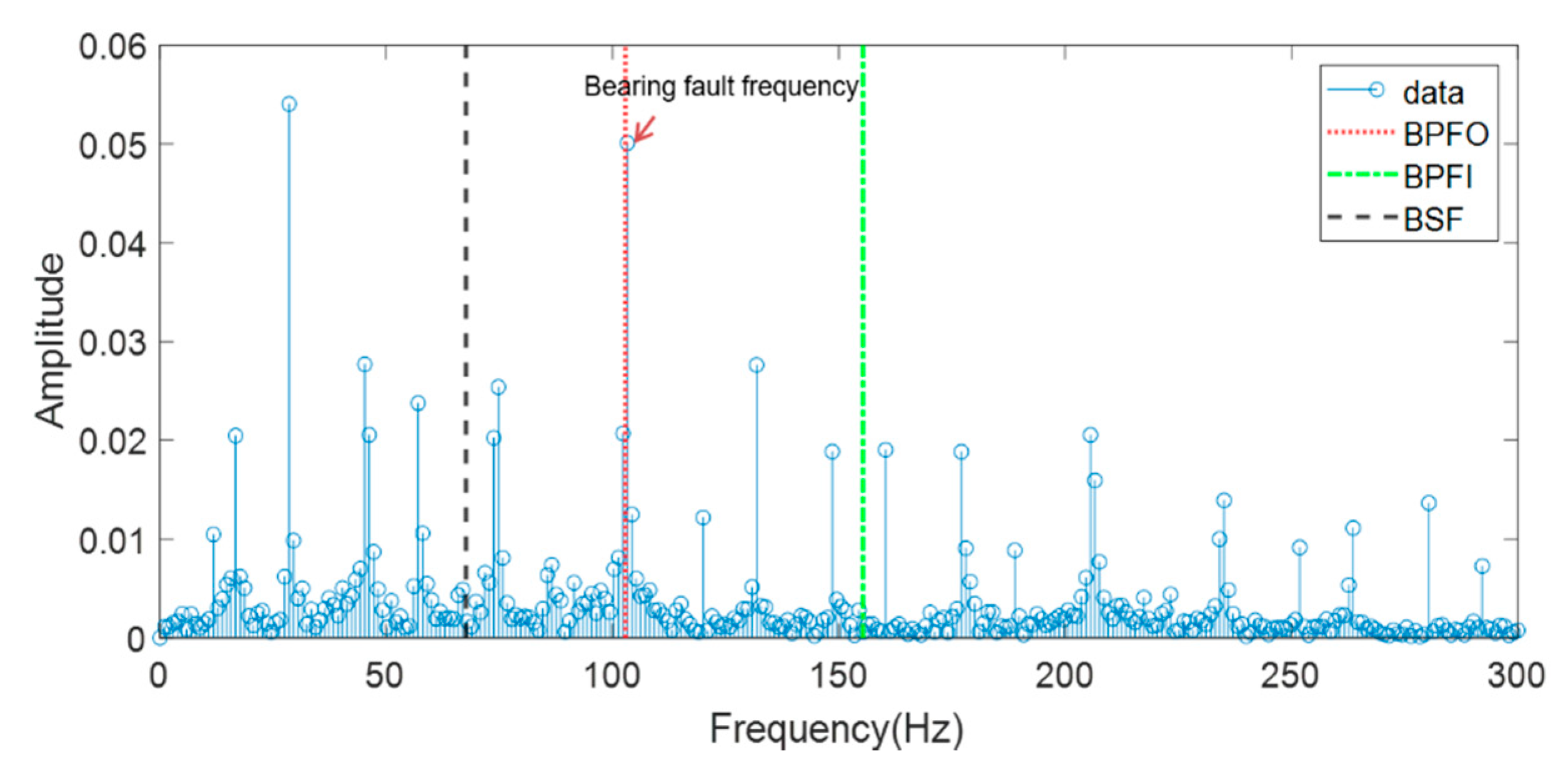
where D, B_D, N_B and α are the bearing diameter, ball diameter, number of the balls, and the contact angle, and w is the rotating frequency of the shaft, respectively. By examining the amplitudes at these frequencies—BPFO, BPFI, and BSF, the fault can be identified in the frequency domain as shown in Figure 6. For example, Figure 8 represents the frequency spectrum after performing fast Fourier transform (FFT) for the envelope signal of CWRU dataset where the outer race was artificially damaged. The peak is apparent at the f_BPFO, proving the presence of fault at the outer race. The corresponding Matlab function to extract the fault frequency features is [feature, feature_name] = Bear_feat(x,fs,bff,cutoff) where bff is the vector of bearing fault frequencies given by Equations (12)–(14), and cutoff is to account for the inaccuracy of these frequencies in the real bearing.

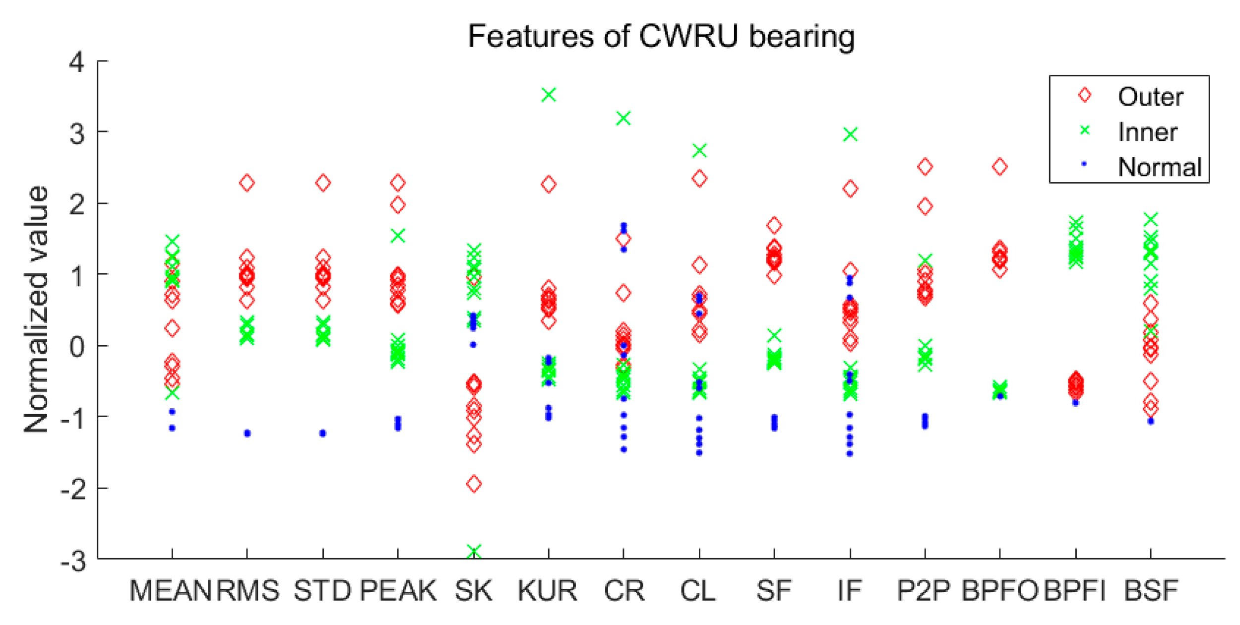
Figure 9 shows the extracted time domain and bearing-specific features altogether for the CWRU bearing dataset: 10 normal, 10 outer race fault, and 10 inner race fault, with each feature normalized by their mean and SD, respectively. While the gear example handled two classes: only the normal and fault, this is a three-class classification: normal, outer and inner, which is more complex for purposes of distinction. Nevertheless, the visual inspection of the results indicates that the RMS, STD, and SF are good classifiers whereas the others are not.

4. Feature Evaluation and Selection for Diagnosis

Feature evaluation is to assess how well the features can classify between the normal and faults. Once this is done, a few numbers of the most significant features can be selected for the efficient fault classification. Although there are many feature evaluation methods for the diagnosis such as Kullback Leibler (KL) divergence, Bhattacharyya distance, features selection by adjusted rand index and standard deviation ratio (FSASR), and support margin local Fisher discriminant ratio (SM-LFDA) [25,26], two of the most popular metrics are introduced in this study to evaluate the performance: Fisher’s discriminant ratio (FDR) and $J_3$, which share the same mathematical background where the former is for the two classes, whereas the latter is for the higher dimensions. Since the HS gear has two classes, it is evaluated by the FDR. The KAUG and CWRU have three classes and are evaluated by the $J_3$.

4.1. Fisher’s Discriminant Ratio

Suppose that the two classes are Gaussian distributed with the mean and standard deviation being ${\mu }_1,{\mu }_2$, and ${\sigma }_1,{\sigma }_2$ respectively. Then, the FDR is defined as follows [25]

$$FDR=\frac{{\left({\mu }_1-{\mu }_2\right)}^2}{{\sigma }_1^2+{\sigma }_2^2},$$

(15)

where the numerator ${\left({\mu }_1-{\mu }_2\right)}^2$ indicates how far the distance is between the centers of two classes, and the denominator ${\sigma }_1^2+{\sigma }_2^2$ indicates how large the dispersion of the two classes is.

Table 3. Rank of FDR value for HS gear.

Top 5	Feature Name	FDR Value	Bottom 5	Feature Name	FDR Value
1	MEAN	57.0285	1	SK	0.0000
2	NB4	15.9001	2	M6A	0.0012
3	M8A	13.0798	3	SER	0.2256
4	FM4	12.9912	4	SF	0.2274
5	CR	12.1305	5	NA4	1.8612

shows the top 5 and bottom 5 FDR values for the total 19 features of HS gear obtained in Figure 4 and Figure 5. Figure 10 shows the probability density functions (PDF) of the MEAN and SK for the two classes, which are those with the highest and lowest FDR values, respectively. Obviously, the MEAN distinguishes the fault from the normal well, whereas the SK does not. These Gaussian PDFs have been obtained by using the mean and standard deviation of the normalized features.

4.2. Scatter Matrices

In the more than two classes problem, the following process should be considered. Denoting the number of classes as M and the prior probability of class as $P_i\cong n_i/N$ where n_i is the number of samples in the ith class and N is the number of total samples, the Within-class scatter matrix, which represents the degree of dispersion within each class, is defined as follows:

$${\mathit{S}}_w={\displaystyle \sum }_{i=1}^M{P}_i{\mathit{S}}_i, where {\mathit{S}}_i=E\left[\left(\mathit{x}-{\mathit{\mu }}_i\right){\left(\mathit{x}-{\mathit{\mu }}_i\right)}^T\right],$$

(16)

where ${\mathit{S}}_i$ is the covariance of the feature vector $\mathit{x}$ with the mean ${\mathit{\mu }}_i$ at the ith class. The Between-class scatter matrix, which represents the distance of the mean of each individual class from the global mean, is then defined as

$${\mathit{S}}_b={\displaystyle \sum }_{i=1}^M{P}_i\left({\mathit{\mu }}_i-{\mathit{\mu }}_0\right){\left({\mathit{\mu }}_i-{\mathit{\mu }}_0\right)}^T, where {\mathit{\mu }}_0={\displaystyle \sum }_{i=1}^M{P}_i{\mathit{\mu }}_i.$$

(17)

The mixture scatter matrix is then defined as

$${\mathit{S}}_m=E\left[\left(\mathit{x}-{\mathit{\mu }}_0\right){\left(\mathit{x}-{\mathit{\mu }}_0\right)}^T\right]={\mathit{S}}_w+{\mathit{S}}_b$$

(18)

With these matrices, a new criterion for feature evaluation is defined as follows [25]:

$$J_3=trace\left\{{\mathit{S}}_w^{-1}{\mathit{S}}_m\right\}$$

(19)

Similar to the FDR, the smaller the ${\mathit{S}}_w$, namely the smaller dispersion within the class, and the larger the ${\mathit{S}}_m$, meaning the larger distance between the different classes, the larger the $J_3$ value we obtain, which means a better classification between the classes. The corresponding Matlab function is in Appendix A as J₃ = ScattMat(data,label) where data are the feature vectors obtained in Section 4 and label is the fault mode. In this study, $J_3$ is calculated to select the two features out of the total features as an illustration. It is applied to the two examples: KAUG and CWRU, which are the three class problems as shown in Table 1. Note in the KAUG problem that the encoder signals are those preprocessed by the TSA. Hence, the 11 time domain features are extracted after applying the HPF only to the signal. Then the $J_3$ are calculated for any two features combinations from 11 features which amount to 55 cases. The features for top 5 and bottom 5 results are listed in

Table 4. Rank of $J_3$ value for KAUG.

Top 5	Feature Combination	${\mathit{J}}_3 \mathbf{Value}$	Bottom 5	Feature Combination	${\mathit{J}}_3 \mathbf{Value}$
1	PEAK & CL	12.341	1	STD & SK	2.2299
2	RMS & IF	12.229	2	RMS & SK	2.2299
3	STD & IF	12.229	3	MEAN & RMS	2.4531
4	PEAK & IF	12.220	4	MEAN & STD	2.4531
5	RMS & CL	12.104	5	RMS & STD	2.4929

. The scatter plot of the best (PEAK & CL) and worst (STD & SK) features are also given in Figure 11a,b, respectively. The differences are outstanding: the features with larger $J_3$ classify the faults much better. In the CWRU problem, the 14 features as shown in Figure 9 are used to find out the two best features based on the $J_3$. The top 5 and bottom 5 results are given in

Table 5. Rank of $J_3$ value for CWRU.

Top 5	Feature Combination	${\mathit{J}}_3 \mathbf{Value}$	Bottom 5	Feature Combination	${\mathit{J}}_3 \mathbf{Value}$
1	SF & P2P	151.38	1	SK & IF	2.5375
2	SF & BPFI	133.34	2	SK & CR	2.5435
3	PEAK & SF	110.48	3	SK & CL	2.6373
4	KUR & SF	108.00	4	KUR & CL	2.8185
5	BPFO & BPFI	100.29	5	KUR & IF	2.9564

. The scatter plots of the two features with best (SF & P2P) and worst (SK & IF) are also given in Figure 12a,b. The same observations are found in this case as well.

5. Feature Evaluation and Selection for Prognosis

This section addresses how to evaluate the predictability performance of the features and select useful ones for the purpose of prognosis. Note that the principle for this is very different from those of diagnosis as the words suggest. The procedure is described via the IMS bearing datasets mentioned in Section 3. Bear in mind that the IMS bearing datasets contain the vibration signals for four bearings, in which dataset 1 contains those of the both (horizontal and vertical) directions for each bearing, whereas datasets 2 and 3 contain only one direction. Among these, the horizontal signal for the bearing #3 of dataset 1 is used for the demonstration, where the inner race is damaged during the experiment. As opposed to the diagnosis where the data are acquired for each discrete class such as the normal, inner race fault and so on, the data in the prognosis are acquired with a certain interval over time for the purpose of monitoring the degradation of the fault. In the IMS bearing, the duration for a single measurement is one second, which are stored in an individual file. They are done by every 5 min for the first 43 numbers, which is followed by every 10 min until failure. In the prognosis, construction of a suitable health index (HI) is necessary, which represents the current health state and enables its monitoring against the failure. The HI can be constructed using the diverse features extracted in the previous section. According to the literature, a good HI is characterized by three metrics: correlation, monotonicity, and robustness in terms of time (or cycles). Higher values of the three metrics give better performance in the prognosis. Therefore, the criterion for feature selection is given by the average of the three metrics in this study.

The first metric for the prognosis is the correlation, which represents the linearity between the features and time:

$$Corr\left(T,X\right)=\frac{cov\left(T,X\right)}{{\sigma }_T{\sigma }_X} ,$$

(20)

where T is time, X is the feature, and σ is the standard deviation over the period. The value toward 1 or −1 means that it has near the perfect linear relationship. The Matlab built-in function for this is Rho = corr(X,Y). Note that this is also called the Pearson correlation. The second metric is the monotonicity, which evaluates the degree of continuous increase or decrease of the feature over time. It is also called Spearman correlation, which is obtained by replacing the variables of the Pearson correlation by its rank variable that represents the standing of the variable in the increasing order:

$$Mon\left(T,X\right)=\frac{cov\left(r{g}_T,r{g}_X\right)}{{\sigma }_{rg}{}_T{\sigma }_{r{g}_X}},$$

(21)

where, rg is the rank of the variables, and σ is its standard deviation. The Matlab built-in function is Rho = corr(X,Y,′Spearman′). Monotonicity also has a value between −1 and 1, of which the absolute value near 1 means that the feature is good for the prognosis. The third metric is the robustness, which has to do with the measurement noise arising in the data acquisition. Because the larger noise can cause poorer performance in the prognosis, selecting features robust to this noise is important. The robustness for this objective is defined as [8]

$$Rob\left(X\right)=\frac{1}{k}{\displaystyle \sum }_k\exp \left(-\left|\frac{X\left(k\right)-\tilde{X}\left(k\right)}{X\left(k\right)}\right|\right),$$

(22)

where $\tilde{X}$ is the smoothed value of X in terms of time. Smoothing is generally conducted by the moving average, which is to average out the current value by the finite number of recent data. It can be obtained by the Matlab built-in function xt = smooth(x). Robustness can be easily calculated by substituting the smoothed data xt in Equation (22).

The three metrics are calculated and averaged for each of the 11 time domain- and 3 bearing- specific features for dataset 1, IMS bearing #3. The results are given in Figure 13a, in which the P2P shows the highest value with 0.749, whereas the SK is the lowest with 0.182. While there are further issues of how to construct a single HI out of these features, this paper ends by representing the trend of the two features over time in Figure 13b,c, in which the P2P shows the distinct increase at around 1800 cycles whereas the SK does not show any trend at all. From this result, it can be concluded that exploiting the metric values in constructing the HI is important for good prognostic performance.

6. Conclusions

While feature engineering is the crucial and practical step for successful PHM, no paper has addressed the basic concepts along with providing the codes for engineers to implement by themselves. The authors have published other tutorial papers with this objective for signal processing [13], which is a very first step, and the particle filter [4], which is the last step of the PHM, respectively. This is another effort towards this end, regarding the feature engineering of the gears and bearings, another preliminary step in order to conduct diagnosis and prognosis. Three public datasets and one dataset by the authors are employed to illustrate the concepts and implement the algorithms via the MATLAB codes given in Appendix A.

References

1. Randall, R.B.; Antoni, J. Rolling element bearing diagnostics—A tutorial. Mech. Syst. Signal. Process. 2011, 25, 485–520. [Google Scholar] [CrossRef]
2. Niu, G. Data-Driven Technology for Engineering Systems Health Management: Design Approach, Feature Construction, Fault Diagnosis, Prognosis, Fusion and Decision; Springer: Beijin, China, 2016; ISBN 9789811020322. [Google Scholar]
3. Lei, Y. Intelligent Fault Diagnosis and Remaining Useful Life Prediction of Rotating Machinery; Elsevier BV: Amsterdam, The Netherlands, 2017. [Google Scholar]
4. An, D.; Choi, J.-H.; Kim, N.H. Prognostics 101: A tutorial for particle filter-based prognostics algorithm using Matlab. Reliab. Eng. Syst. Saf. 2013, 115, 161–169. [Google Scholar] [CrossRef]
5. Vachtsevanos, G.; Lewis, F.; Roemer, M.; Hess, A.; Wu, B. Intelligent Fault Diagnosis and Prognosis for Engineering Systems; Wiley: Hoboken, NJ, USA, 2006. [Google Scholar]
6. Goodman, D.; Hofmeister, J.P.; Szidarovszky, F. Prognostics and Health Management: A Practical Approach to Improve System Reliability Using Condition-Based Data; Wiley: New York City, NY, USA, 2019; ISBN 9781119356691. [Google Scholar]
7. Lee, J.; Wu, F.; Zhao, W.; Ghaffari, M.; Liao, L.; Siegel, D. Prognostics and health management design for rotary machinery systems—Reviews, methodology and applications. Mech. Syst. Signal Process. 2014, 42, 314–334. [Google Scholar] [CrossRef]
8. Lei, Y.; Li, N.; Guo, L.; Li, N.; Yan, T.; Lin, J. Machinery health prognostics: A systematic review from data acquisition to RUL prediction. Mech. Syst. Signal Process. 2018, 104, 799–834. [Google Scholar] [CrossRef]
9. Jardine, A.K.; Lin, D.; Banjevic, D. A review on machinery diagnostics and prognostics implementing condition-based maintenance. Mech. Syst. Signal Process. 2006, 20, 1483–1510. [Google Scholar] [CrossRef]
10. Faulstich, S.; Hahn, B.; Tavner, P.J. Wind turbine downtime and its importance for offshore deployment. Wind. Energy 2011, 14, 327–337. [Google Scholar] [CrossRef]
11. Kim, S.; Choi, J.-H. Convolutional neural network for gear fault diagnosis based on signal segmentation approach. Struct. Health Monit. 2018, 18, 1401–1415. [Google Scholar] [CrossRef]
12. Ham, S.; Han, S.-Y.; Kim, S.; Park, H.J.; Park, K.-J.; Choi, J.-H. A Comparative Study of Fault Diagnosis for Train Door System: Traditional versus Deep Learning Approaches. Sensors 2019, 19, 5160. [Google Scholar] [CrossRef] [PubMed] [Green Version]
13. Kim, S.; Lim, C.; Ham, S.-J.; Park, H.; Choi, J.-H. Tutorial for Prognostics and Health Management of Gears and Bearings: Advanced Signal Processing Technique. Trans. Korean Soc. Mech. Eng. A 2018, 42, 1119–1131. [Google Scholar] [CrossRef]
14. Bechhoefer, E. High Speed Gear Dataset. Available online: https://www.kau-sdol.com/kaug (accessed on 10 December 2019).
15. Bearing Data Center, Case Western Reserve University. Available online: https://csegroups.case.edu/bearingdatacenter/pages/download-data-file (accessed on 10 December 2019).
16. Lee, J.; Qiu, H.; Yu, G.; Lin, J. Rexnord Technical Services IMS Bearing Data. Available online: https://ti.arc.nasa.gov/c/3/ (accessed on 13 August 2020).
17. Caesarendra, W. Vibration and Acoustic Emission-Based Condition Monitoring and Prognostic Methods for Very Low Speed Slew Bearing. Ph.D. Thesis, University of Wollongong, Wollongong, Australia, 2015. [Google Scholar]
18. Lei, Y.; Zuo, M.J. Gear crack level identification based on weighted K nearest neighbor classification algorithm. Mech. Syst. Signal Process. 2009, 23, 1535–1547. [Google Scholar] [CrossRef]
19. Lebold, M.; McClintic, K.; Campbell, R.; Byington, C.; Maynard, K. Review of vibration analysis methods for gearbox diagnostics and prognostics. In Proceedings of the 54th Meeting of the Society for Machinery Failure Prevention Technology, Virginia Beach, VA, USA, 1–4 May 2000; pp. 623–634. [Google Scholar]
20. Pattabiraman, T.R.; Srinivasan, K.; Malarmohan, K. Assessment of sideband energy ratio technique in detection of wind turbine gear defects. Case Stud. Mech. Syst. Signal Process. 2015, 2, 1–11. [Google Scholar] [CrossRef] [Green Version]
21. Decker, H.J.; Lewicki, D.G. Spiral Bevel Pinion Crack Detection in a Helicopter Gearbox. In Proceedings of the American Helicopter Society 59th Annual Forum, Phoenix, AZ, USA, 6–8 May 2003; pp. 1222–1232. [Google Scholar]
22. Sreejith, B.; Verma, A.K.; Srividya, A. Fault diagnosis of rolling element bearing using time-domain features and neural networks. In Proceedings of the 2008 IEEE Region 10 and the Third international Conference on Industrial and Information Systems, Kharagpur, India, 8–10 December 2008; pp. 1–6. [Google Scholar]
23. Hanna, J.; Hatch, C.; Kalb, M.; Weiss, A.; Luo, H. Detection of Wind Turbine Gear Tooth Defects Using Sideband Energy Ratio. In Proceedings of the China Wind Power 2011, Beijing, China, 19–21 October 2011. [Google Scholar]
24. Park, J.; Kim, S.; Choi, J.-H.; Lee, S.H. Frequency energy shift method for bearing fault prognosis using microphone sensor. Mech. Syst. Signal Process. 2021, 147, 107068. [Google Scholar] [CrossRef]
25. Theodoridis, S.; Koutroumbas, K. Pattern Recognition, 2nd ed.; Elsevier Science: San Diego, CA, USA, 2003; ISBN 9780080513621. [Google Scholar]
26. Yu, X.; Dong, F.; Ding, E.; Wu, S.; Fan, C. Rolling Bearing Fault Diagnosis Using Modified LFDA and EMD with Sensitive Feature Selection. IEEE Access 2018, 6, 3715–3730. [Google Scholar] [CrossRef]
Figure 1. Framework of Prognostics and health management (PHM).
Applsci 10 05639 g001
Figure 2. Overall procedure of traditional versus deep learning-based diagnostics [11].
Applsci 10 05639 g002
Figure 3. Features extraction process for gears.
Applsci 10 05639 g003
Figure 4. Normalized time domain features of high speed (HS) gears.
Applsci 10 05639 g004
Figure 5. Normalized gear specific features of HS gear.
Applsci 10 05639 g005
Figure 6. Features extraction process for bearing.
Applsci 10 05639 g006
Figure 7. Bearing geometry.
Applsci 10 05639 g007
Figure 8. Frequency domain data of CWRU outer race fault bearing.
Applsci 10 05639 g008
Figure 9. General time domain features and bearing specific features of CWRU bearing.
Applsci 10 05639 g009
Figure 10. PDF of (a) MEAN, and (b) SK, representing the max and min FDR, respectively, for HS gear.
Applsci 10 05639 g010
Figure 11. Scatter plot of two features with (a) max J 3 and (b) min J 3 for KAUG.
Applsci 10 05639 g011
Figure 12. Scatter plot of two features with (a) max J 3 and (b) min J 3 for CWRU bearing.
Applsci 10 05639 g012
Figure 13. Feature evaluation of IMS bearing dataset 1 bearing #3, (a) calculated feature selection criteria, (b) best feature for prognosis, (c) worst feature for prognosis.
Applsci 10 05639 g013