Bearing Fault Identification Using Machine Learning and Adaptive Cascade Fault Observer

Abstract

In this work, a hybrid procedure for bearing fault identification using a machine learning and adaptive cascade observer is explained. To design an adaptive cascade observer, the normal signal approximation is the first step. Therefore, the fuzzy orthonormal regressive (FOR) technique was developed to approximate the acoustic emission (AE) and vibration (non-stationary and nonlinear) bearing signals in normal conditions. After approximating the normal signal of bearing using the FOR technique, the adaptive cascade observer is modeled in four steps. First, the linear observation technique using a FOR proportional-integral (PI) observer (FOR-PIO) is developed. In the second step, to increase the power of uncertaintie rejection (robustness) of the FOR-PIO, the structure procedure is used serially. Next, the fuzzy like observer is selected to increase the accuracy of FOR structure PI observer (FOR-SPIO). Moreover, the adaptive technique is used to develop the reliability of the cascade (fuzzy-structure PI) observer. Additionally to fault identification, the machine-learning algorithm using a support vector machine (SVM) is recommended. The effectiveness of the adaptive cascade observer with the SVM fault identifier was validated by a vibration and AE datasets. Based on the results, the average vibration and AE fault diagnosis using the adaptive cascade observer with the SVM fault identifier are 97.8% and 97.65%, respectively.

1. Introduction

Most countries are currently facing energy-related challenges. Generally, fossil fuels are a major source of energy in most countries. However, the use of fossil fuels causes many problems, such as greenhouse gas emissions like CO₂. In recent years, we have produced about 29 gigatons of CO₂ annually, and around 40% of this can be absorbed naturally. Therefore, we have issues with around 60% of the CO₂ we produce. Increasing CO₂ in the atmosphere causes several challenges, such as global warming and pollution. Heavy industries have played a large role in increasing the emission rate of CO₂. Numerous components are used in heavy industries, including various types of motors. Several factors can be analyzed in attempts to increase the efficiency of motors. Among these, condition monitoring and fault diagnosis of motors are important methods that can be taken advantage of to increase efficiency and reduce CO₂ emissions. Various kinds of faults have been introduced for motors, which can be divided into two main categories: (a) mechanical faults, such as bearing faults (around 69% of faults) and the other types of mechanical faults (around 10%) and (b) electrical faults (around 21%). Bearings are clearly a significant component in motors. Inner race faults (IRF), outer race faults (ORF), and ball faults (BLF) are the main fault types in bearings. Various kinds of condition monitoring have been used for fault diagnosis of bearings, such as methods based on vibration analysis, acoustic emission (AE) analysis, lubricant/debris analysis, power quality analysis and microscope analysis, and motor current signature analysis (MCSA) [1].

Various procedures have been recommended for fault diagnosis in bearings, including techniques based on signal processing procedures, methods based on data-driven techniques, techniques using model-based approaches, and mixtures of the above techniques using hybrid approaches [2,3,4,5,6,7,8]. Regarding the advantages of signal processing techniques, they have some challenges when used in uncertain conditions. Additionally, data-driven approaches have some limitations when used with large datasets, and model-based techniques have limitations in terms of accurate system modeling. To address the above issues a hybrid technique is recommended in this work. To analyze the vibration and AE signals, the signal processing techniques play an important role. A system with a bearing fault is identified as a complex nonlinear and non-stationary one [9]. Due to these issues and the limitation of the conventional time- and frequency-domain analysis, the researchers and engineers are forced to define two scenarios: (a) utilize complex time-frequency analysis (TFA) methods, and (b) utilize the hybrid approach for extracting valuable information about the mechanical fault and performing fault diagnosis. The most frequently used TFAs are empirical mode decomposition (EMD) [10] and its derivative methods, such as ensemble EMD (EEMD) [11,12], and wavelet transform with its variations [13,14,15]. Apart from various positive points of these techniques for fault diagnosis in the bearing, these methods suffer some drawbacks in real industries including mode-mixing in the EMD [16], computational complexity in the EEMD, energy leakage and interference terms, and selection of the mother wavelet function the wavelet transform [17,18,19]. Due to the complexity and the problems of TFA signal analysis techniques for extracting discriminative fault features as well as the problems of the classical machine learning methods which are dependent on the quality of the feature, two scenarios have been recommended by researchers and engineers: the family of (machine/deep) learning approaches and the family of modern control algorithms. The (machine/deep) learning techniques can be used for fault feature extraction and including convolutional neural networks [20,21,22,23,24,25,26] to autonomously extract the features, generative adversarial networks [27] to generate the new signals that resemble the original ones, different types of autoencoders [28,29] for latent coding for signal reconstruction; generation; compression; anomaly detection, and deep neural network (DNN) [30] to increase the performance of classification accuracy in high-dimensional and uncertain input data. The second scenario is the modern control-based algorithm for fault feature identification. The observation-based approach is one of the powerful techniques in the family of modern control algorithms and can be classified into two main categories: linear and nonlinear observers. The modern control procedures using linear observers have been used in real industries. The main issues of these techniques are robustness and reliability. To address these issues, two different scenarios have been defined by researchers: nonlinear-based observers that have the challenge of complexities and hybrid approaches. Various kinds of hybrid approaches have been reported in [31,32,33,34]. The first step to develop a hybrid observer is a function approximation [35]. Although function approximation using a mathematical approach is reliable, it has two important problems: high complexity and low accuracy in uncertain conditions [36,37,38]. System identification techniques are the next scenario for function approximation. Several system identification techniques have been used for function approximation such as auto-regressive with external inputs (ARX), ARX-Laguerre, and intelligent-based ARX-Laguerre techniques [35,36,39].

To estimate the different classes of signals using observers, diverse methods have been introduced such as sliding mode, feedback linearization, backstepping, fuzzy, and proportional-integral (PI) observers [40,41,42]. High reliability and robustness are the main characteristics of sliding mode observer, but the most important negative characteristics of this technique are high-frequency fluctuation and complexity [41,43]. The second scenario to estimate the unknown signal is the feedback linearization observer. A lack of robustness and complexity are the main negative characteristics of this technique [44]. To address the issues of complexity of implementation for sliding mode and feedback linearization observers, the PI observer was developed. Implementing this technique is simple, but the main drawbacks of this technique are estimation accuracy and resistance, especially when the signal is non-stationary. The ARX-Laguerre PI observer technique was recommended in [36,39,45] to improve the accuracy estimation. The extended technique has been recommended to solve the challenge of robustness in the ARX-Laguerre PI observer [39]. The ARX-Laguerre procedure does not provide a favorable result when dealing with the complex, non-stationary, and nonlinear faults that occur in rotating machinery. In this work, this issue is addressed by proposing a fuzzy orthonormal regressive technique. After approximating the normal signal of bearing using the fuzzy orthonormal regressive, the adaptive cascade observer is developed in four steps. First, the linear observation technique using a proportional-integral (PI) observer with the fuzzy orthonormal regressive signal approximation is developed. In the second step, to increase the power of uncertainties rejection in the PI observer, the structure procedure is used serially. Next, the fuzzy like observer is selected to increase the accuracy of structure PI observer. Moreover, the adaptive technique is used to develop the reliability of the cascade (fuzzy-structure PI) observer. Therefore, in this work, an adaptive cascade observer is recommended for highly accurate signal estimation.

After approximating the normal signal function using a fuzzy orthonormal regressive method and estimating the signals using an adaptive cascade observer, the residual signals are generated and faults can be classified. Moreover, the residual signals are calculated by the difference between various conditions of the original signals and estimated signals obtained using an adaptive cascade observer. Since the adaptive cascade observer is tuned for working in the normal condition, the estimated signal is generated by the proposed adaptive cascade observer with minimum error for normal states. However, in the abnormal condition, the accuracy of signal estimation is reduced. Therefore, the difference between original signal and estimated signal in the abnormal condition will increase. In addition, the residual signals can be used as high discriminative features for fault detection and diagnosis of bearing. These residual signals are used at the next step as the input for machine learning technique to perform fault identification and the values of the residual of signals for adaptive cascade observer. In this work, we employ a machine learning technique for classification of the faults using the support vector machines (SVM) algorithm [46] to complete the proposed hybrid adaptive cascade fault diagnosis method. The SVM is known as a robust machine learning algorithm that is insensitive to the curse of dimensionality problem [47]. One of the main advantages of the SVM is that it can be efficiently applied for classification of both linear and nonlinear-separable types of datasets which is possible due to the availability of different types of kernels, such as linear, polynomial, and radial basis function kernels [48]. However, despite its flexibility, several challenges in this classifier should be addressed to obtain the best possible performance on the target task. Specifically, the first challenge is the selection of the kernel function itself. This is an important step since it directly affects the performance of the classifier when applied to the specific dataset. The kernel selection dilemma can be resolved by applying the prior knowledge about the data being analyzed (i.e., whether it is linearly separable or not) or the kernel can be selected experimentally by trial and error. The second challenge, which is also closely related to the first one, is the selection of the hyperparameter values which is dependent on the kernel type. In this paper, the linear kernel was selected for the SVM classifier experimentally because it demonstrated the most accurate separation of the features belonging to different classes in the dataset used. The conventional grid search algorithm was applied to fine-tune its hyperparameter value (i.e., the maximum distance for the boundary).

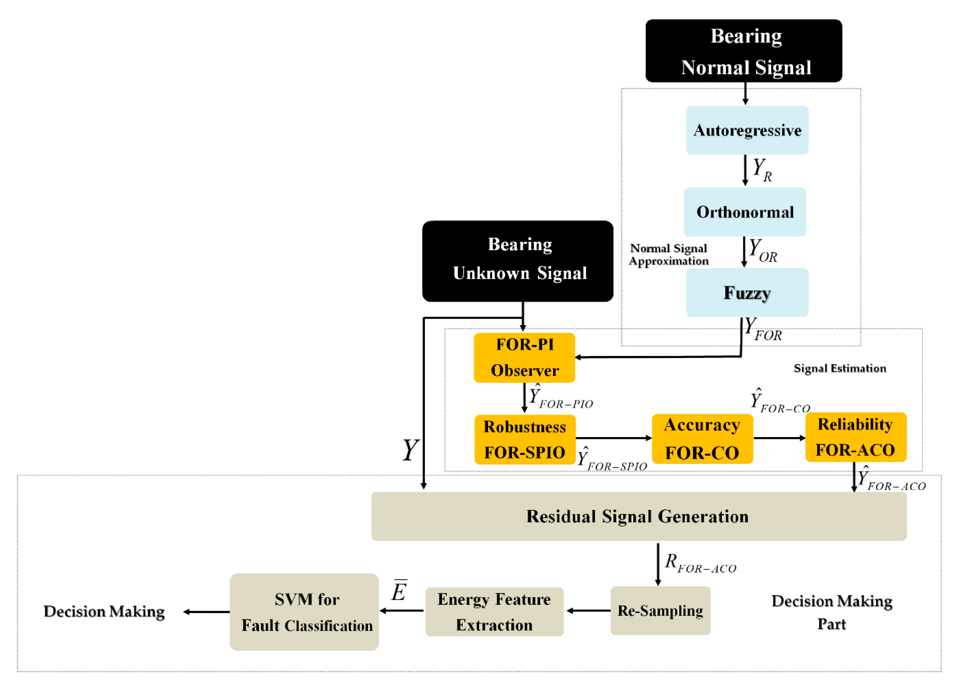
Figure 1 illustrates the block diagram of the adaptive cascade observer with the SVM method for fault diagnosis in rotary machinery. According to this figure, this method has three main blocks: signal approximation using fuzzy orthonormal regressive (FOR), signal estimation using a FOR-adaptive cascade observer (FOR-ACO), and fault decision using SVM. For signal approximation, in the first step, a regressive technique is proposed. To increase the strength of resistance to disturbances in the regressive technique, the orthonormal regressive is used in the next step. Besides, to increase the accuracy of the signal approximation, the fuzzy orthonormal regressive technique (FOR) is developed. After approximating the normal signal using the FOR technique, the FOR-PI observer (FOR-PIO) fault estimation is developed. This technique presents two important challenges: low robustness and high estimation error. The structure fault observer is proposed to modify the robustness of FOR-PIO. Moreover, the fuzzy logic algorithm is represented to reduce the signal estimation error in FOR-SPIO. Additionally, the adaptive technique is proposed to improve the reliability of the cascade observer. The decision-making part has three sub-blocks: residual generation; windows characterization and energy feature extraction; fault classification using the SVM algorithm.

Three main contributions in this research are listed as follows:

• Normal signal approximation for time-series normal signal using fuzzy orthonormal regressive technique.
• Developing an adaptive cascade observer for signal estimation.
• Improving the performance of the classification technique by generating the residual signals, extracting the features of energy from them, and applying to SVM for fault identification.

The remainder of this manuscript is organized as follows. The second section outlines the datasets. The third section outlines the fuzzy orthonormal regressive signal approximation. The adaptive cascade observer with SVM for unknown signal classification is represented in Section 4. In the next section, verification of the adaptive cascade method with the SVM fault classifier is analyzed. In the last section, conclusions are explained.

2. Experimental Datasets

To test the effectiveness of the adaptive cascade observer and SVM technique, two datasets are represented:

• The Case Western Reserve University (CWRU) vibration bearing dataset to test the single fault diagnosis accuracy.

  Table 1. Case Western Reserve University (CWRU) Vibration Datasets.

  Datasets	Conditions	Load (hp)	Crack Sizes (in)
  A	NRM	0	0.007, 0.014, and 0.021
  	BLF	0
  	IRF	0
  	ORF	0
  B	NRM	1	0.007, 0.014, and 0.021
  	BLF	1
  	IRF	1
  	ORF	1
  C	NRM	2	0.007, 0.014, and 0.021
  	BLF	2
  	IRF	2
  	ORF	2
  D	NRM	3	0.007, 0.014, and 0.021
  	BLF	3
  	IRF	3
  	ORF	3

  shows information related to the vibration CWRU bearing dataset [1,49]. A 2-hp motor is used to rotate the bearing in the various rotational speeds and a vibration sensor is used to collect the normal and abnormal data in 48 kHz. This dataset has four classes such as normal (NRM), ball fault (BLF), inner fault (IRF), and outer fault (ORF). In addition, the crack sizes in the abnormal conditions are 0.007, 0.014, and 0.021 inches in diameter, respectively.
• The Ulsan Industrial Artificial Intelligence (UIAI) Lab AE bearing dataset is used as a second dataset to test the power of adaptive cascade with SVM technique for multiple fault identification.

  Table 2. Ulsan Industrial Artificial Intelligence (UIAI) Lab Acoustic Emission Bearing Datasets.

  Datasets	Faults	Motor (RPM)	Crack Sizes (mm)
  A	NRM	300	3 and 6
  	IRF	300
  	ORF	300
  	BLF	300
  	IRF-ORF	300
  	IRF-BLF	300
  	ORF-BLF	300
  	IRF-ORF-BLF	300
  B	NRM	400	3 and 6
  	IRF	400
  	ORF	400
  	BLF	400
  	IRF-ORF	400
  	IRF-BLF	400
  	ORF-BLF	400
  	IRF-ORF-BLF	400
  C	NRM	450	3 and 6
  	IRF	450
  	ORF	450
  	BLF	450
  	IRF-ORF	450
  	IRF-BLF	450
  	ORF-BLF	450
  	IRF-ORF-BLF	450
  D	NRM	500	3 and 6
  	IRF	500
  	ORF	500
  	BLF	500
  	IRF-ORF	500
  	IRF-BLF	500
  	ORF-BLF	500
  	IRF-ORF-BLF	500

  shows the information of UIAI dataset [39]. This dataset has eight classes, such as normal (NRM), ball fault (BLF), inner fault (IRF), outer fault (ORF), inner-ball fault (IRF-BLF), outer-ball fault (ORF-BLF), inner-outer fault (IRF-ORF), and inner-outer-ball fault (IRF-ORF-BLF) conditions. This motor is working under four rotational speeds, such as 300, 400, 450, and 500 RPM. In addition, the crack sizes are 3 and 6 mm in diameter.

3. Normal Signal of Bearing Approximation Using Fuzzy Orthonormal Regressive Technique

Designing the observer for nonlinear and nonstationary signals is a vital challenge. Therefore, to develop an observer, normal signal of bearing approximation using the time-series identification technique is the first step. In this work, we develop the fuzzy orthonormal regressive procedure. Based on Figure 1, the orthonormal regressive technique is implemented to approximate and extract the state-space equation from the bearing signals. Moreover, the orthonormal regressive approach is selected to improve the robustness of the state-space bearing function approximation. Finally, the error of the state-space bearing model can be reduced using the fuzzy orthonormal regressive technique. The regressive (R) algorithm for approximate the REB vibration and AE normal signals is [36,45]:

$$Y_R\left(k\right)={\sum }_{i=1}^{{\delta }_Y}{\complement }_Y\left(i\right)Y_R\left(k-i\right)+{\sum }_{i=1}^{{\delta }_{U_i}}{\complement }_{U_i}\left(i\right)U_i\left(k-i\right),$$

(1)

where $Y_R\left(k\right),U_i\left(k\right),\left({\complement }_x\left(i\right),{\complement }_y\left(i\right)\right)$, and $\left({\delta }_{U_i},{\delta }_Y\right)$ are the normal bearing signal approximation using the R-technique, the uncertainties for REB signal approximation, parameters to tune the function approximation, and the order of the function approximation technique, respectively. To increase the resistance of the modeled regressive function against uncertainties and disturbance, the orthonormal regressive (OR) procedure is used.

The state-space equation using the OR technique to model the REB is:

$$Y_{OR}\left(k\right)={\displaystyle \sum _{n=0}^{i_Y-1}}{\complement }_Y\left(i\right){\overline{O}}_{n,Y_{OR}}\left(k,{\gamma }_Y\right)Y_{OR}\left(k-i\right)+{\displaystyle \sum _{n=0}^{i_{U_i}-1}}{\complement }_{U_i}\left(i\right){\overline{O}}_{n,U_i}\left(k,{\gamma }_{U_i}\right)U_i\left(k-i\right)$$

(2)

Here, $Y_{OR}\left(k\right),{\overline{O}}_{n,Y_{OR}}\left(k,{\gamma }_Y\right)$, and ${\overline{O}}_{n,U_i}\left(k,{\gamma }_{U_i}\right)$ are the normal bearing signal approximation using the OR technique, the function of orthonormal, and the orthonormal of uncertain condition for REB, respectively. The accuracy of the normal signal approximation is an important factor for function approximation. To reduce the signal approximation error and increase the nonlinear approximation accuracy, the fuzzy technique is recommended. Generally, the fuzzy algorithm can be introduced using the following definition:

$$if\langle I_1\rangle is\langle L{V}_1\rangle and\langle I_2\rangle is\langle L{V}_2\rangle then\langle O\rangle is\langle L{V}_O\rangle .$$

(3)

Here, $\langle I_1\rangle \mathrm{and}\langle I_2\rangle ,\langle L{V}_1\rangle \mathrm{and}\langle L{V}_2\rangle ,\langle O\rangle ,$ and $\langle L{V}_O\rangle$ are fuzzy logic input signals, linguistic variables for input signals, the fuzzy logic output signal, and the linguistic variable for the fuzzy logic output signal, respectively. Thus, the state-space function approximation for normal bearing signal using fuzzy orthonormal regressive (FOR) is represented using Equation (4).

$$\{\begin{array}{c}{X}_{FOR}\left(k+1\right)=\left[{\sigma }_X{X}_{FOR}\left(k\right)+{\sigma }_Y{Y}_{FOR}\left(k\right)+{\sigma }_U{U}_i\left(k\right)\right]+{\sigma }_F{\varnothing }_F\left(k\right)\\ Y_{FOR}\left(k\right)={\left(\beta \right)}^T{X}_{FOR}\left(k\right)\end{array}$$

(4)

Here, $X_{FOR}\left(k\right), Y_{FOR}\left(k\right), {\varnothing }_F\left(k\right)$, and $\left({\sigma }_X,{\sigma }_Y,{\sigma }_U,\beta ,{\sigma }_F\right)$ are the state of normal signal approximation for REB using the fuzzy orthonormal regressive technique, the output function of normal signal approximation for REB using the fuzzy orthonormal regressive technique, the fuzzy parameter used to reduce the error of signal approximation, and parameters to adjust the signal approximation function, respectively. To find the error of the function approximation using the FOR technique, the following formulation is used.

$$e_{FOR}\left(k\right)=Y_o\left(k\right)-Y_{FOR}\left(k\right).$$

(5)

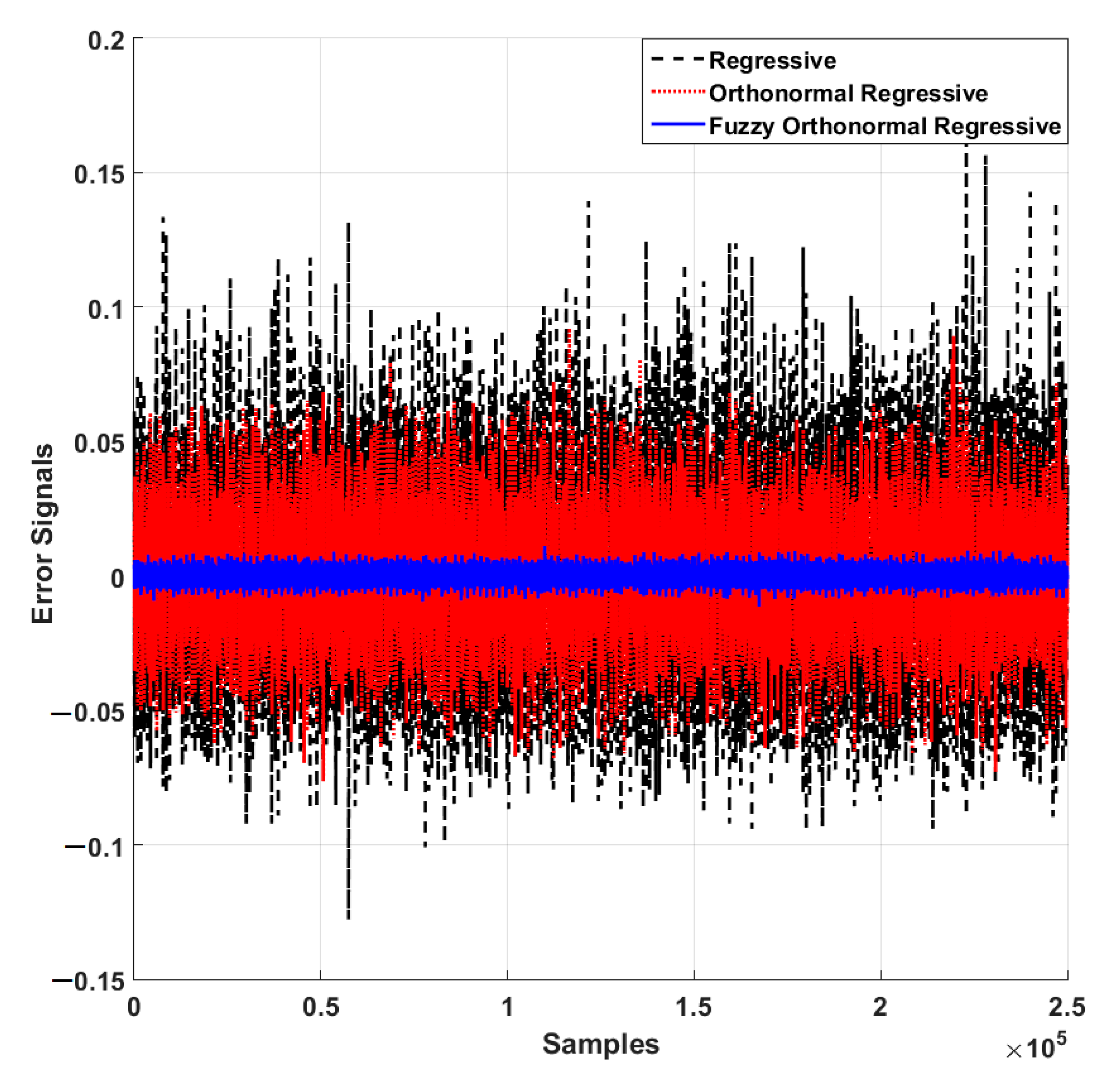
Here, $e_{FOR}\left(k\right)$ and $Y_o\left(k\right)$ are the error of the function approximation using FOR technique and the original normal (RAW) signal, respectively. Figure 2 illustrates the comparison between the error of function approximation using the regressive (R) technique, the orthonormal regressive (OR) algorithm, and the FOR procedure. Regarding this figure, the accuracy of the FOR technique is higher than others. Consequently, this technique is more suitable to evaluate the adaptive cascade observer, which is used for signal estimation.

4. Adaptive Cascade Observer with Machine Learning for Fault Identification

After finding the state-space equation for the normal signal function approximation part, the adaptive cascade observer for unknown signal estimation is developed. This Section has two main sub-sections: (a) development of the adaptive cascade observer for unknown signal estimation, and (b) generating the residual signals, extracting the energy features from those signals to evaluate the highly accurate technique for fault identification using the SVM technique.

4.1. Adaptive Cascade Observer for Signal Estimation

To modify the bearing signal estimation accuracy, the adaptive cascade observer is recommended. The cascade observer is developed using the fuzzy-structure PI observer and the fuzzy orthonormal regressive technique is used to approximate the normal signal. Based on Figure 1, the adaptive cascade observer follows four steps: (a) establish a linear observer using an PI observer and FOR normal signal approximation, (b) the structure fault observer is used to increase the resistance of the PI observer against uncertainties such as rotational speed variation or torque load variation, (c) the fuzzy logic algorithm is used to improve the accuracy of the structure PI observer and develop cascade observer, and (d) the adaptive algorithm is used for auto tuning and important parameter of cascade observer using fuzzy logic technique. The first step of cascade observer using PI observation technique and FOR normal signal approximation is represented using the Equations (6) and (7):

$$\{\begin{array}{c}\begin{array}{c}{\widehat{X}}_{FOR-PIO}\left(k+1\right)=\left[{\sigma }_X{\widehat{X}}_{FOR-PIO}\left(k\right)+{\sigma }_Y{\widehat{Y}}_{FOR-PIO}\left(k\right)+{\sigma }_U{U}_i\left(k\right)\right]+{\widehat{\phi }}_{FOR-PIO}\left(k\right)+\\ {\sigma }_1\times e_{FOR-PIO}\end{array}\\ {\widehat{Y}}_{FOR-PIO}\left(k\right)={\left(\beta \right)}^T{\widehat{X}}_{FOR-PIO}\left(k\right)\\ e_{FOR-PIO}=X_{FOR}\left(k\right)-{\widehat{X}}_{FOR-PIO}\left(k\right)\\ e_{r-FOR-PIO}=Y_o\left(k\right)-{\widehat{Y}}_{FOR-PIO}\left(k\right)\end{array}$$

(6)

To improve the uncertainties accuracy in PI observer with FOR normal signal approximation, the following technique is developed.

$${\widehat{\phi }}_{FOR-PIO}\left(k+1\right)={\widehat{\phi }}_{FOR-PIO}\left(k\right)+{\sigma }_2\times e_{r-FOR-PIO}.$$

(7)

Here, ${\widehat{X}}_{FOR-PIO}\left(k\right),{\widehat{ Y}}_{FOR-PIO}\left(k\right), {\widehat{\phi }}_{FOR-PIO}\left(k\right), Y_o\left(k\right)$, and $\left({\sigma }_1,{\sigma }_2\right)$ are the state estimation using the PI observer with FOR normal signal approximation, the estimation of the unknown signals using the PI observer with FOR normal signal approximation, unknown condition (the speed or torque variant) observation using the PI observer with FOR normal signal approximation, the original signal, and the coefficients, respectively. Notwithstanding, this technique is easy to implement, in unknown conditions the accuracy is reduced. Thus, the structure fault observer is established to increase the resistance of the PI observer against uncertainties such as rotational speed variation or torque load variation. Moreover, the structure PI observer with FOR normal signal approximation is defined as follows.

$$\{\begin{array}{c}\begin{array}{c}{\widehat{X}}_{FOR-SPIO}\left(k+1\right)=\left[{\sigma }_X{\widehat{X}}_{FOR-SPIO}\left(k\right)+{\sigma }_Y{\widehat{Y}}_{FOR-SPIO}\left(k\right)+{\sigma }_U{U}_i\left(k\right)\right]+{\widehat{\phi }}_{FOR-SPIO}\left(k\right)+\\ {\sigma }_1\times e_{FOR-SPIO}\end{array}\\ {\widehat{Y}}_{FOR-SPIO}\left(k\right)={\left(\beta \right)}^T{\widehat{X}}_{FOR-SPIO}\left(k\right)\\ e_{FOR-SPIO}=X_{FOR}\left(k\right)-{\widehat{X}}_{FOR-SPIO}\left(k\right)\\ e_{r-FOR-SPIO}=Y_o\left(k\right)-{\widehat{Y}}_{FOR-SPIO}\left(k\right)\end{array}$$

(8)

That, the ${\widehat{\phi }}_{FOR-SPIO}\left(k\right)$ is defined as follows.

$${\widehat{\phi }}_{FOR-SPIO}\left(k+1\right)={\widehat{\phi }}_{FOR-SPIO}\left(k\right)+{\sigma }_2\times e_{r-FOR-SPIO}+{\sigma }_3.sgn\times e_{r-FOR-SPIO}$$

(9)

Here, ${\widehat{X}}_{FOR-SPIO}\left(k\right), {\widehat{Y}}_{FOR-SPIO}\left(k\right), {\widehat{\phi }}_{FOR-SPIO}\left(k\right)$, and ${\sigma }_3$ are the state estimation using the structure PI observer with FOR normal signal approximation, the estimation of the unknown signals using the structure PI observer with FOR normal signal approximation, unknown condition (the speed or torque variant) observation using the structure PI observer with FOR normal signal approximation, and the variable structure surface coefficient, respectively. Next, the fuzzy logic algorithm is used to improve the accuracy of the structure PI observer and develop cascade observer. Therefore, to modify the efficiency in the structure PI observer with FOR normal signal approximation, the fuzzy logic approach is developed here. First, the T-S fuzzy logic approach is defined as follows.

$$if{e}_{FOR-fSPIO}\left(k\right)isThthen{\widehat{\phi }}_f\left(k+1\right)={\widehat{\phi }}_f\left(k\right)+{\sigma }_f\times e_{FOR-fSPIO}.$$

(10)

Here, $e_{FOR-fSPIO}\left(k\right), Th,{\widehat{\phi }}_f\left(k\right)$, and ${\sigma }_f$ are the error of estimation based on the cascade observer with FOR normal signal approximation, the threshold level for tuning, the T-S fuzzy estimation function, and fuzzy logic tuning parameter, respectively. Based on Equation (10), the cascade observer with FOR normal signal approximation is developed by Equations (11) and (12).

$$\{\begin{array}{c}\begin{array}{c}{\widehat{X}}_{FOR-fSPIO}\left(k+1\right)=\left[{\sigma }_X{\widehat{X}}_{FOR-CO}\left(k\right)+{\sigma }_Y{\widehat{Y}}_{FOR-CO}\left(k\right)+{\sigma }_U{U}_i\left(k\right)\right]+{\widehat{\phi }}_{FOR-CO}\left(k\right)+\\ {\sigma }_1\times e_{FOR-CO}\end{array}\\ {\widehat{Y}}_{FOR-CO}\left(k+1\right)={\left(\beta \right)}^T{\widehat{X}}_{FOR-CO}\left(k\right)\\ e_{FOR-CO}=X_{A-L}\left(k\right)-{\widehat{X}}_{FOR-CO}\left(k\right)\\ e_{r-FOR-CO}=Y_o\left(k\right)-{\widehat{Y}}_{FOR-CO}\left(k\right)\end{array}.$$

(11)

That, the ${\widehat{\phi }}_{FOR-CO}\left(k\right)$ is defined as follows.

$${\widehat{\phi }}_{FOR-CO}\left(k+1\right)={\widehat{\phi }}_{FOR-CO}\left(k\right)+{\sigma }_2\times e_{r-FOR-CO}+{\sigma }_3.sgn\times e_{FOR-r-CO}+{\sigma }_4\times {\widehat{\phi }}_f\left(k\right).$$

(12)

Here, ${\widehat{X}}_{FOR-CO}\left(k\right), {\widehat{Y}}_{FOR-CO}\left(k\right),{\widehat{ \phi }}_{FOR-CO}\left(k\right)$, and ${\sigma }_4$ are state estimation using the fuzzy logic structure PI (cascade) observer with FOR normal signal approximation, the estimation of the unknown signals using the cascade observer with FOR normal signal approximation, unknown condition (motor speed variant) estimation using the cascade observer with FOR normal signal approximation, and the constant for tuning the fuzzy parameters of function, respectively.

To increase the reliability and accuracy of bearing signal estimation in normal condition, the adaptive (online tuning) technique is developed to auto-tune the important coefficient. For auto-tuning the coefficient of robust function, the fuzzy logic algorithm is recommended. This definition is provided below.

$${\sigma }_{3-adaptive}={\sigma }_3\times \theta .$$

(13)

Therefore, the improved cascade observer using adaptive technique is expressed as follows:

$$\{\begin{array}{c}\begin{array}{c}{\widehat{X}}_{FOR-ACO}\left(k+1\right)=\left[{\sigma }_X{\widehat{X}}_{FOR-ACO}\left(k\right)+{\sigma }_Y{\widehat{Y}}_{FOR-ACO}\left(k\right)+{\sigma }_U{U}_i\left(k\right)\right]+{\widehat{\phi }}_{FOR-ACO}\left(k\right)+\\ +{\sigma }_1\times e_{FOR-ACO}\end{array}\\ {\widehat{Y}}_{FOR-ACO}\left(k+1\right)={\left(\beta \right)}^T{\widehat{X}}_{FOR-ACO}\left(k\right)\\ e_{FOR-ACO}=X_{A-L}\left(k\right)-{\widehat{X}}_{FOR-ACO}\left(k\right)\\ e_{r-FOR-ACO}=Y_o\left(k\right)-{\widehat{Y}}_{FOR-ACO}\left(k\right)\end{array},$$

(14)

$$\begin{array}{c}{\widehat{\phi }}_{FOR-ACO}\left(k+1\right)={\widehat{\phi }}_{FOR-ACO}\left(k\right)+{\sigma }_2\times e_{r-FOR-ACO}+\\ {\sigma }_{3-adaptive}.sgn\times e_{FOR-r-ACO}+{\sigma }_4\times {\widehat{\phi }}_f\left(k\right).\end{array}$$

(15)

Here, ${\widehat{X}}_{FOR-ACO}\left(k\right), {\widehat{Y}}_{FOR-ACO}\left(k\right),{\widehat{ \phi }}_{FOR-ACO}\left(k\right), \theta$, and ${\sigma }_{3-adaptive}$ state estimation using the adaptive cascade observer with FOR normal signal approximation, the estimation of the unknown signals using the adaptive cascade observer with FOR normal signal approximation, unknown condition (motor speed variant) estimation using the adaptive cascade observer with FOR normal signal approximation, the adaptive auto-tuning parameter using the fuzzy algorithm, and the auto-tuned coefficient using the adaptive technique, respectively. Therefore, due to Figure 1 and Equations (14) and (15), the adaptive cascade observer is developed to estimate the unknown vibration and AE signals of a bearing. The stability and robustness for proposed algorithm are proof in the Appendix A. Next, the residual signal is generated, and the energy features are extracted from residual signals for fault identification using machine learning.

4.2. Fault Detection and Classification Using SVM

In the previous section, the signal was estimated using the adaptive cascade observer. Additionally, the residual signals for the adaptive cascade observer with FOR normal signal approximation $\left(r_{FOR-r-ACO}\left(k\right)\right)$ is defined by the following functions, respectively.

$$r_{FOR-r-ACO}\left(k\right)=Y_o\left(k\right)-{\widehat{Y}}_{FOR-ACO}\left(k\right).$$

(16)

Figure 3 illustrates the residual signals for the REB vibration dataset using the adaptive cascade observer. Regarding this figure, it is clear that the adaptive cascade observation technique for signal estimation obtained differentiable signals for fault diagnosis.

After calculating the residual signals, in the next step, the energy signals are extracted from the residual signals. These signals are used for classification algorithm using SVM. Therefore, the energy signals $\left(\overline{E}\right)$ extracted from the residual signals is calculated as follows.

$$\overline{E}={\displaystyle \sum }_{i=1}^K{r}_{FOR-r-ACO-i}{}^2.$$

(17)

Here, $r_{FOR-r-ACO-i}$ is the $ith$ sample of the residual signal obtained by the adaptive cascade observer and $K$ is the number of samples. The features of energy that are extracted from the residual signals for the CWRU dataset using adaptive cascade observer are shown in Figure 4. Since the adaptive cascade observer is tuned for working in the normal condition, the amplitude of the energy of the residual signal is reduced. However, in the abnormal condition, the accuracy of signal estimation is reduced. Therefore, the energy of residual signal in the abnormal condition is increased. Thus, after determining the energy of residual signals using Equations (16) and (17) as a high discriminative feature, the machine learning algorithm using support vector machine (SVM) is selected for identification the faults in the bearing. This technique is a mathematical-based algorithm and used for classification. The soft margin SVM is selected according the following definition [34,50].

$$w_i\left({\varnothing }^T\rho (q_i)+c\right)\ge w_i-v_i.$$

(18)

Here, $\left(q_i, w_i\right), \left(\varnothing ,c\right), \rho \left(q_i\right),$ and $v_i$ are the SVM inputs, the SVM outputs, features that are used in SVM, and maximum distance for boundary, respectively. The primal algorithm is used to solve Equation (18) and defined as follows.

$$\begin{array}{c}\begin{array}{cc}min& \frac{1}{2}\end{array}{\varnothing }^T\varnothing +\rho {\displaystyle {\displaystyle \sum }_i}{v}_i\\ \begin{array}{cc}s.t.& \begin{array}{cc}{w}_i\left({\varnothing }^T\rho (q_i)+c\right)\ge w_i-v_i& v_i\ge 0\end{array}\end{array}\end{array}$$

(19)

Here, $\rho$ is a penalty to tuning the boundary of SVM. To solve this equation, the minmax (saddle) point is defined based on the following equation.

$$M{M}_p=\frac{1}{2}{\varnothing }^T\varnothing +\rho {\displaystyle \sum }_i{v}_i-{\displaystyle \sum }_i{\partial }_i\left[w_i\left({\varnothing }^T\rho (q_i)+c\right)-w_i+v_i\right]-{\displaystyle \sum }_i{\sigma }_i{v}_i$$

(20)

where $M{M}_p$ and $({\partial }_i,{\sigma }_i)$ are the minmax point and the saddle function coefficients, respectively. To maximize the saddle point, $({\partial }_i,{\sigma }_i)$ and to minimize it $\left(\varnothing , v_i,c\right)$ have an essential role. To solve the minmax challenge the quadratic programming is represented. Therefore, the ${\partial }_i$ is represented as follows:

$$\begin{array}{cc}min& \frac{1}{2}{\partial }^{T}K\partial +H^T\partial \\ s.t.& \begin{array}{c}{\displaystyle {\displaystyle \sum }_i}{\partial }_i{w}_i=0\\ \begin{array}{cc}0\le {\partial }_i\le \rho & \forall i\end{array}\end{array}\end{array}$$

(21)

Here, $H=\left[\begin{array}{c}-1\\ -1\\ \begin{array}{c}⋮\\ -1\end{array}\end{array}\right]$. Next, the other parameters $\left(\varnothing , c\right)$ are represented as:

$$\varnothing ={\displaystyle \sum }_i{\partial }_i{w}_{i}K\left(x_i,x\right)$$

(22)

$$c=\frac{1}{\left|SV\right|}{\displaystyle \sum }_{i\in SV}(w_i-{\displaystyle \sum }_j{\partial }_j{w}_{j}K\left(x_i,x_j\right))$$

(23)

Here $K\left(x_i,x_j\right)$ and $SV$ are kernel function which is defined as a nonlinear function and support vector, respectively. In Equation (23), the support vector is represented as:

$$SV=\left\{i|0\le v_i\le \rho \right\}$$

(24)

Finally, the SVM with nonlinear function is represented as:

$$w_i=sgn({\displaystyle \sum }_i{\partial }_i{w}_{i}K\left(x_i,x_j\right)+c)$$

(25)

The FOR-adaptive cascade observer and SVM technique for fault classification are detailed in Algorithm 1.

Algorithm 1. The adaptive cascade observation technique for fault diagnosis in a bearing
1:	Approximate the normal signal using FOR technique (4)
2:	Estimate the signal based on the FOR-PI observer (FOR-PIO) (6,7)
3:	Improve the power of uncertain and unknown condition rejection using FOR-SPI observer (FOR-SPIO) (8,9)
4:	Increase the accuracy using FOR-cascade observer (10–12)
5:	The reliability and stability are improved using FOR-adaptive cascade observer (FOR-ACO) (13–15)
6:	Residual signal is generated using Equation (16)
7:	The energy feature is extracted from residual signal using Equation (17)
8:	The signal and fault are classified using SVM (25)

5. Experimental Results

To test the effectiveness of bearing fault identification using the FOR-adaptive cascade observer (FOR-ACO), this procedure is validated and compared with two state-of-the-art techniques: the FOR-SPIO and the FOR-PIO. Additionally, the CWRU vibration signal is used to test the power of single-type fault classification and UIAI-Lab acoustic emission signal is selected to test the power of multi-type fault identification in crack-variant and load-variant conditions.

Table 3. Window Characterization for Training and Testing: CWRU Data.

Classes	Four, (NRM, IRF, ORF, BLF)
Samples Per Classes	400
Training Samples	1200 (300 samples per classes)
Testing Samples	400 (100 samples per classes)

and

Table 4. Window Characterization for Training and Testing: SHSE Lab Dataset.

Classes	Eight, (NRM, IRF, ORF, BLF, IRF-ORF, IRF-BLF, ORF-BLF, IRF-ORF-BLF)
Samples Per Classes	800
Training Samples	2400 (300 samples per classes)
Testing Samples	800 (100 samples per classes)

illustrate the window characterization for training and testing samples for CWRU and UIAI-Lab datasets, respectively.

5.1. CWRU Dataset

In this section, the SVM is directly applied to FOR-ACO, FOR-SPIO, and FOR-PIO that further are referred to as SVM + FOR-ACO, SVM + FOR-SPIO, and SVM + FOR-PIO, respectively. These methods are used to test single-type fault identification in two different conditions: crack-variant and load-variant conditions.

5.1.1. Vibration Crack-Variant CWRU Dataset

First, we investigate the fault identification capabilities of the SVM + FOR-ACO, the SVM + FOR-SPIO, and the SVM + FOR-PIO on four vibration crack-variant datasets provided by CWRU. For these investigations, the torque load remains fixed and the average accuracy (ACA) values are exposed in

Table 5. The Accuracy of Single-Type Fault Identification When the Torque Load is 0-hp.

Techniques	SVM + FOR-ACO			SVM + FOR-SPIO			SVM + FOR-PIO
Crack Sizes (inch)	0.007	0.014	0.021	0.007	0.014	0.021	0.007	0.014	0.021
NRM	100%	100%	100%	100%	100%	100%	88%	88%	88%
BLF	96%	96%	97%	93%	93%	94%	88%	78%	78%
ORF	87%	93%	95%	80%	93%	96%	75%	81%	78%
IRF	96%	96%	97%	95%	93%	93%	70%	70%	71%
ACA	94.8%	96.3%	97.3%	92%	94.8%	95.7%	80.3%	79.3%	78.8%

,

Table 6. The Accuracy of Single-Type Fault Identification When the Torque Load is 1-hp.

Techniques	SVM + FOR-ACO			SVM + FOR-SPIO			SVM + FOR-PIO
Crack Sizes (inch)	0.007	0.014	0.021	0.007	0.014	0.021	0.007	0.014	0.021
NRM	100%	100%	100%	100%	100%	100%	88%	88%	88%
BLF	97%	97%	99%	95%	93%	95%	80%	81%	85%
ORF	98%	98%	99%	91%	91%	93%	78%	80%	81%
IRF	95%	90%	96%	91%	93%	96%	70%	74%	75%
ACA	97.5%	96.3%	98.5%	94.3%	94.3%	96%	79%	80.8%	82.3%

,

Table 7. The Accuracy of Single-Type Fault Identification When the Torque Load is 2-hp.

Techniques	SVM + FOR-ACO			SVM + FOR-SPIO			SVM + FOR-PIO
Crack Sizes (inch)	0.007	0.014	0.021	0.007	0.014	0.021	0.007	0.014	0.021
NRM	100%	100%	100%	100%	100%	100%	85%	85%	85%
BLF	95%	95%	96%	93%	93%	96%	79%	81%	84%
ORF	97%	97%	98%	95%	90%	90%	79%	75%	80%
IRF	96%	98%	99%	95%	94%	94%	75%	76%	79%
ACA	97%	97.5%	93.3%	95.8%	94.3%	95%	79.5%	79.3%	82%

and

Table 8. The Accuracy of Single-Type Fault Identification When the Torque Load is 3-hp.

Techniques	SVM + FOR-ACO			SVM + FOR-SPIO			SVM + FOR-PIO
Crack Sizes (inch)	0.007	0.014	0.021	0.007	0.014	0.021	0.007	0.014	0.021
NRM	100%	100%	100%	100%	100%	100%	90%	90%	90%
BLF	95%	97%	100%	91%	90%	91%	79%	79%	80%
ORF	96%	97%	100%	90%	90%	94%	76%	78%	80%
IRF	94%	97%	100%	90%	91%	91%	75%	77%	79%
ACA	96.3%	97.8%	100%	92.8%	92.8%	94%	80%	81%	82.3%

.

Based on these tables, the SVM + FOR-ACO (proposed scheme) outperforms the SVM + FOR-SPIO and SVM + FOR-PIO for fault identification in bearing. Moreover, the average accuracy of fault classification for the SVM + FOR-ACO is about 96.7%, while the SVM + SOR-SPIO and SVM + FOR-PIO show accuracy values of 94.3% and 80.3%, respectively. Besides, the SVM+FOR-ACO outperforms the SVM + FOR-SPIO, yielding, on average, the accuracy of identification improved by about 2.7%, 3%, and 1.1% for 0.007, 0.014, and 0.021-inch crack sizes, respectively. Additionally, the SVM + FOR-ACO outperforms the SVM + FOR-PIO, yielding, on average, the accuracy of identification improved by about 16.7%, 16.9%, and 15% for 0.007, 0.014, and 0.021 inch crack sizes, respectively.

5.1.2. Vibration Load-Variant CWRU Dataset

To validate the reliability, stability, and robustness, we investigated the fault identification capabilities of the SVM + FOR-ACO, the SVM + FOR-SPIO, and the SVM + FOR-PIO on the vibration load-variant datasets provided by CWRU when the cracks remain fixed. The average accuracy values (ACA) are shown in the following table (

Table 9. The Accuracy of Single-Type Fault Identification to Test the Load-Variant Dataset.

Techniques	SVM + FOR-ACO			SVM + FOR-SPIO			SVM + FOR-PIO
Crack Sizes (inch)	0.007	0.014	0.021	0.007	0.014	0.021	0.007	0.014	0.021
NRM	100%	100%	100%	100%	100%	100%	91%	91%	88%
BLF	96%	97%	97%	91%	90%	91%	80%	81%	83%
ORF	87%	93%	94%	87%	90%	90%	73%	75%	79%
IRF	94%	97%	97%	90%	92%	92%	80%	84%	84%
ACA	97.8%	96.8%	97%	92%	93%	93.3%	81%	82.8%	83.5%

).

Concerning this table, the average accuracy of the identification of the degradation for the SVM + FOR-ACO, which was used to validate the robustness, is about 97.2%. For the SVM + FOR-SPIO method, it is about 92.8%, and for the SVM + FOR-PIO plan, it is about 82.4%. Furthermore, the SVM + FOR-ACO outperforms the SVM + FOR-SPIO, yielding, on average, the accuracy of identification improved by about 5.8%, 3.8%, and 3.7% for 0.007, 0.014, and 0.021 inch crack sizes, respectively. Moreover, the SVM + FOR-ACO also outperforms the SVM + FOR-PIO, yielding, on average, the accuracy of identification improved by about 16.8%, 14%, and 13.5% for 0.007, 0.014, and 0.021 inch crack sizes, respectively. Regarding the power of the SVM + FOR-ACO for single-type fault detection and classification of a bearing for crack-variant and load-variant tests, the SVM + FOR-ACO is more persuasive than the other two schemes.

5.2. UIAI-Lab Dataset

In the second scenario, the SVM + FOR-ACO, SVM + FOR-SPIO, and SVM + FOR-PIO are used to test multi-type fault identification in two different conditions: crack-variant and load-variant conditions.

5.2.1. Acoustic Emission Crack-Variant UIAI-Lab Dataset

Now, we investigate the fault identification capabilities of the SVM + FOR-ACO, the SVM + FOR-SPIO, and the SVM + FOR-PIO on AE crack-variant datasets provided by UIAI-Lab. For these investigations, the torque speed remains fixed, crack sizes are 3 and 6 mm. The ACA values are exposed in

Table 10. The Accuracy of Multi-Type Fault Identification When the Torque Speed is 300 RPM.

Techniques	SVM + FOR-ACO		SVM + FOR-SPIO		SVM + FOR-PIO
Crack Sizes (mm)	3	6	3	6	3	6
NRM	100%	100%	100%	100%	83%	83%
IRF	94%	95%	93%	94%	69%	73%
ORF	96%	97%	95%	95%	71%	75%
BLF	97%	97%	94%	94%	78%	77%
IRF-BLF	98%	98%	93%	96%	79%	81%
ORF-BLF	99%	99%	95%	97%	80%	80%
IRF-ORF	96%	96%	94%	94%	78%	82%
IRF-ORF-BLF	98%	99%	95%	96%	78%	80%
ACA%	97.3	97.6	94.9	95.8	77	77.9

,

Table 11. The Accuracy of Multi-Type Fault Identification When the Torque Speed is 400 RPM.

Techniques	SVM + FOR-ACO		SVM + FOR-SPIO		SVM + FOR-PIO
Crack Sizes (mm)	3	6	3	6	3	6
NRM	100%	100%	100%	100%	86%	86%
IRF	97%	98%	94%	96%	73%	73%
ORF	97%	98%	93%	93%	71%	78%
BLF	98%	98%	95%	94%	76%	77%
IRF-BLF	98%	98%	95%	96%	80%	83%
ORF-BLF	96%	97%	94%	95%	83%	84%
IRF-ORF	96%	97%	98%	96%	78%	80%
IRF-ORF-BLF	97%	98%	96%	95%	78%	79%
ACA%	97.4	98	95.5	95.6	78.1	80

,

Table 12. The Accuracy of Multi-Type Fault Identification When the Torque Speed is 450-RPM.

Techniques	SVM + FOR-ACO		SVM + FOR-SPIO		SVM + FOR-PIO
Crack Sizes (mm)	3	6	3	6	3	6
NRM	100%	100%	100%	100%	88%	88%
IRF	97%	98%	94%	94%	74%	74%
ORF	97%	97%	95%	94%	76%	78%
BLF	98%	98%	94%	95%	80%	80%
IRF-BLF	98%	96%	93%	95%	80%	81%
ORF-BLF	97%	98%	94%	94%	79%	78%
IRF-ORF	98%	98%	96%	97%	80%	81%
IRF-ORF-BLF	96%	97%	95%	96%	80%	80%
ACA%	97.7	97.7	95.1	95.6	79.6	80

and

Table 13. The Accuracy of Multi-type Fault Identification When the Torque Speed is 500 RPM.

Techniques	SVM + FOR-ACO		SVM + FOR-SPIO		SVM + FOR-PIO
Crack Sizes (mm)	3	6	3	6	3	6
NRM	100%	100%	100%	100%	88%	88%
IRF	97%	98%	95%	95%	80%	80%
ORF	97%	99%	96%	94%	78%	80%
BLF	98%	98%	97%	96%	81%	83%
IRF-BLF	98%	99%	94%	94%	82%	84%
ORF-BLF	98%	97%	95%	95%	85%	84%
IRF-ORF	97%	98%	94%	96%	80%	82%
IRF-ORF-BLF	97%	97%	95%	96%	81%	81%
ACA%	97.8	98.3	95.8	95.6	81.9	82.8

.

Based on Table 10, Table 11, Table 12 and Table 13, the SVM + FOR-ACO (proposed scheme) outperforms the SVM + FOR-SPIO and SVM + FOR-PIO for fault identification in bearing. Moreover, the average accuracy of fault classification for the SVM + FOR-ACO is about 97.8%, while the SVM + SOR-SPIO and SVM + FOR-PIO show accuracy values of 95.5% and 79.7%, respectively. Besides, the SVM + FOR-ACO outperforms the SVM + FOR-SPIO, yielding, on average, the accuracy of identification improved by about 2.3% and 2.2% for 3 and 6 mm crack sizes, respectively. Furthermore, the SVM + FOR-ACO outperforms the SVM + FOR-PIO, yielding, on average the accuracy of identification improved by about 18.4% and 17.7% for 3 and 6 mm crack sizes, respectively.

5.2.2. Acoustic Emission Load-Variant UIAI-Lab Datasets

To validate the reliability, stability, and robustness, we investigated the fault identification capabilities of the SVM + FOR-ACO, the SVM + FOR-SPIO, and the SVM + FOR-PIO on the AE load-variant datasets provided by UIAI-Lab when the cracks remain fixed. The ACA values are shown in the following table (

Table 14. The Accuracy of Multi-Type Fault Identification to Test the Motor Speed-Variant Dataset.

Techniques	SVM + FOR-ACO		SVM + FOR-SPIO		SVM + FOR-PIO
Crack Sizes (mm)	3	6	3	6	3	6
NRM	100%	100%	100%	100%	86%	86%
IRF	98%	96%	90%	90%	80%	80%
ORF	96%	97%	92%	94%	75%	78%
BLF	96%	99%	94%	95%	80%	81%
IRF-BLF	97%	98%	93%	96%	80%	86%
ORF-BLF	98%	98%	96%	94%	84%	85%
IRF-ORF	98%	97%	94%	94%	80%	82%
IRF-ORF-BLF	97%	97%	94%	95%	80%	83%
ACA%	97.5	97.8	94.1	94.8	80.6	82.6

). Concerning this table, the average accuracy of the identification of the degradation for the SVM + FOR-ACO, which was used to validate the robustness, is about 97.65%. For the SVM + FOR-SPIO method, it is about 94.45%, and for the SVM + FOR-PIO plan, it is about 81.6%. Additionally, the SVM + FOR-ACO outperforms the SVM + FOR-SPIO, yielding, on average, the accuracy of identification improved by about 3.4% and 3% for 3 and 6 mm crack sizes, respectively. Moreover, the SVM + FOR-ACO also outperforms the SVM + FOR-PIO, yielding, on average, the accuracy of identification improved by about 16.9% and 15.2% for 3 and 6 mm crack sizes, respectively. Regarding the power of the SVM+FOR-ACO for multi-type fault identification of a bearing for crack-variant and load-variant tests, the SVM+FOR-ACO is more persuasive than the other two schemes.

6. Conclusions

In this paper, an adaptive cascade observer with SVM technique was developed for fault identification of rotating machinery. This algorithm was industrialized using the following steps: (a) time-series signal approximation using the fuzzy orthonormal regressive (FOR) technique, (b) signal estimation using an adaptive cascade observer, and (c) fault identification using the SVM technique. The fuzzy orthonormal regressive technique was developed to model the AE and vibration (non-stationary and nonlinear) bearing signals in normal conditions to develop a high-accuracy observer. Moreover, to obtain accurate classification of the signals in various conditions, an adaptive cascade observer was developed. Therefore, the linear observation technique using a FOR proportional-integral (PI) observer (FOR-PIO) was developed in the initial step. After that, to increase the power of uncertainties rejection in the FOR-PIO, the structure procedure was settled. Next, to improve the performance of FOR-structure PI observer (FOR-SPIO) the fuzzy like observer was selected and the developed cascade observer. Moreover, the adaptive technique was selected to develop the reliability of the cascade observer and the developed FOR-adaptive cascade observer (FOR-ACO). Additionally, the fault was identified by support vector machine (SVM). The effectiveness of the adaptive cascade observer with the SVM fault identifier was validated by a vibration and AE datasets. Regarding the results, the average vibration and AE fault diagnosis using the FOR-ACO with the SVM fault identifier are 97.8% and 97.65%, respectively. In the future, the parallel deep-learning technique will be used to improve the accuracy and flexibility of the cascade observers.

References

1. Adams, M.L. Analysis of Rolling Element Bearing Faults in Rotating Machinery: Experiments, Modeling, Fault Detection and Diagnosis; Case Western Reserve University: Cleveland, OH, USA, 2001. [Google Scholar]
2. Cecati, C. A Survey of Fault Diagnosis and Fault-Tolerant Techniques—Part II: Fault Diagnosis With Knowledge-Based and Hybrid/Active Approaches. IEEE Trans. Ind. Electron. 2015, 62, 1. [Google Scholar]
3. Gao, Z.; Cecati, C.; Ding, S.X. A survey of fault diagnosis and fault-tolerant techniques—Part I: Fault diagnosis with model-based and signal-based approaches. IEEE Trans. Ind. Electron. 2015, 62, 3757–3767. [Google Scholar] [CrossRef] [Green Version]
4. Liu, Z.; Liu, T.; Han, J.; Bu, S.; Tang, X.; Pecht, M. Signal model-based fault coding for diagnostics and prognostics of analog electronic circuits. IEEE Trans. Ind. Electron. 2016, 64, 605–614. [Google Scholar] [CrossRef]
5. Ahmad, W.; Khan, S.A.; Kim, J.-M. A hybrid prognostics technique for rolling element bearings using adaptive predictive models. IEEE Trans. Ind. Electron. 2017, 65, 1577–1584. [Google Scholar] [CrossRef]
6. Glowacz, A. Acoustic-based fault diagnosis of commutator motor. Electronics 2018, 7, 299. [Google Scholar] [CrossRef] [Green Version]
7. Huo, Z.; Zhang, Y.; Shu, L.; Gallimore, M. A new bearing fault diagnosis method based on fine-to-coarse multiscale permutation entropy, laplacian score and SVM. IEEE Access 2019, 7, 17050–17066. [Google Scholar] [CrossRef]
8. Chu, Z.; Meng, F.; Zhu, D.; Luo, C. Fault reconstruction using a terminal sliding mode observer for a class of second-order MIMO uncertain nonlinear systems. ISA Trans. 2020, 97, 67–75. [Google Scholar] [CrossRef]
9. Chu, F.; Lu, W. Experimental observation of nonlinear vibrations in a rub-impact rotor system. J. Sound Vib. 2005, 283, 621–643. [Google Scholar] [CrossRef]
10. Cheng, J.; Yu, D.; Tang, J.; Yang, Y. Local rub-impact fault diagnosis of the rotor systems based on EMD. Mech. Mach. Theory 2009, 44, 784–791. [Google Scholar] [CrossRef]
11. Prosvirin, A.E.; Islam, M.M.M.; Kim, J.-M. An Improved Algorithm for Selecting IMF Components in Ensemble Empirical Mode Decomposition for Domain of Rub-Impact Fault Diagnosis. IEEE Access 2019, 7, 121728–121741. [Google Scholar] [CrossRef]
12. Lei, Y.; He, Z.; Zi, Y. Application of the EEMD method to rotor fault diagnosis of rotating machinery. Mech. Syst. Signal Process. 2009, 23, 1327–1338. [Google Scholar] [CrossRef]
13. Zhihao, J.; Shangwei, J.; Wen, J.; Bangchun, W. Rubbing Fault Diagnosis of Rotary Machinery Based on Wavelet and Support Vector Machine; IEEE: Piscataway, NJ, USA, 2009; pp. 287–290. [Google Scholar]
14. Lu, Y.; Meng, F.; Li, Y. Research on Rub Impact Fault Diagnosis Method of Rotating Machinery Based on Wavelet Packet and Support Vector Machine. In Proceedings of the 2009 International Conference on Measuring Technology and Mechatronics Automation, Zhangjiajie, China, 11–12 April 2009; pp. 707–710. [Google Scholar]
15. Roy, S.D.; Shome, S.K.; Laha, S.K. Impact of wavelets and filter on vibration-based mechanical rub detection using Neural Networks. In Proceedings of the 2014 Annual IEEE India Conference (INDICON), Pune, India, 11–13 December 2014; pp. 1–6. [Google Scholar]
16. Lei, Y.; Lin, J.; He, Z.; Zuo, M.J. A review on empirical mode decomposition in fault diagnosis of rotating machinery. Mech. Syst. Signal Process. 2013, 35, 108–126. [Google Scholar] [CrossRef]
17. Tse, P.W.; Yang, W.; Tam, H.Y. Machine fault diagnosis through an effective exact wavelet analysis. J. Sound Vib. 2004, 277, 1005–1024. [Google Scholar] [CrossRef]
18. Bessous, N.; Zouzou, S.E.; Bentrah, W.; Sbaa, S.; Sahraoui, M. Diagnosis of bearing defects in induction motors using discrete wavelet transform. Int. J. Syst. Assur. Eng. Manag. 2018, 9, 335–343. [Google Scholar] [CrossRef]
19. Bessam, B.; Menacer, A.; Boumehraz, M.; Cherif, H. Wavelet transform and neural network techniques for inter-turn short circuit diagnosis and location in induction motor. Int. J. Syst. Assur. Eng. Manag. 2017, 8, 478–488. [Google Scholar] [CrossRef]
20. Krizhevsky, A.; Sutskever, I.; Hinton, G.E. ImageNet classification with deep convolutional neural networks. Commun. ACM 2017, 60, 84–90. [Google Scholar] [CrossRef]
21. Moeskops, P.; Viergever, M.A.; Mendrik, A.M.; de Vries, L.S.; Benders, M.J.N.L.; Isgum, I. Automatic Segmentation of MR Brain Images With a Convolutional Neural Network. IEEE Trans. Med Imaging 2016, 35, 1252–1261. [Google Scholar] [CrossRef] [Green Version]
22. Arab, D.M.; Benmoussa, S.; Zio, E. Review on Health Indices Extraction and Trend Modeling for Remaining Useful Life Estimation. In Artificial Intelligence Techniques for a Scalable Energy Transition; Springer: Cham, Switzerland, 2020; pp. 183–223. [Google Scholar]
23. Liu, R.; Meng, G.; Yang, B.; Sun, C.; Chen, X. Dislocated Time Series Convolutional Neural Architecture: An Intelligent Fault Diagnosis Approach for Electric Machine. IEEE Trans. Ind. Inform. 2017, 13, 1310–1320. [Google Scholar] [CrossRef]
24. Appana, D.K.; Prosvirin, A.; Kim, J.-M. Reliable fault diagnosis of bearings with varying rotational speeds using envelope spectrum and convolution neural networks. Soft Comput. 2018, 22, 6719–6729. [Google Scholar] [CrossRef]
25. Wu, X.; Peng, Z.; Ren, J.; Cheng, C.; Zhang, W.; Wang, D. Rub-Impact Fault Diagnosis of Rotating Machinery Based on 1-D Convolutional Neural Networks. IEEE Sens. J. 2020, 20, 8349–8363. [Google Scholar] [CrossRef]
26. Chen, X.; Kopsaftopoulos, F.; Wu, Q.; Ren, H.; Chang, F.-K. A Self-Adaptive 1D Convolutional Neural Network for Flight-State Identification. Sensors 2019, 19, 275. [Google Scholar] [CrossRef] [PubMed] [Green Version]
27. Khan, S.A.; Prosvirin, A.E.; Kim, J.-M. Towards bearing health prognosis using generative adversarial networks: Modeling bearing degradation. In Proceedings of the 2018 International Conference on Advancements in Computational Sciences (ICACS), Lahore, Pakistan, 19–21 February 2018; pp. 1–6. [Google Scholar]
28. Principi, E.; Rossetti, D.; Squartini, S.; Piazza, F. Unsupervised electric motor fault detection by using deep autoencoders. IEEE/CAA J. Autom. Sin. 2019, 6, 441–451. [Google Scholar] [CrossRef]
29. Jiang, G.; He, H.; Xie, P.; Tang, Y. Stacked Multilevel-Denoising Autoencoders: A New Representation Learning Approach for Wind Turbine Gearbox Fault Diagnosis. IEEE Trans. Instrum. Meas. 2017, 66, 2391–2402. [Google Scholar] [CrossRef]
30. Chen, Z.; Li, Z. Research on fault diagnosis method of rotating machinery based on deep learning. In Proceedings of the 2017 Prognostics and System Health Management Conference (PHM-Harbin), Harbin, China, 9–12 July 2017; pp. 1–4. [Google Scholar]
31. Xue, X.; Zhou, J. A hybrid fault diagnosis approach based on mixed-domain state features for rotating machinery. ISA Trans. 2017, 66, 284–295. [Google Scholar] [CrossRef] [PubMed]
32. Ahmed, H.O.; Nandi, A.K. Three-stage hybrid fault diagnosis for rolling bearings with compressively sampled data and subspace learning techniques. IEEE Trans. Ind. Electron. 2018, 66, 5516–5524. [Google Scholar] [CrossRef] [Green Version]
33. Zhou, S.; Qian, S.; Chang, W.; Xiao, Y.; Cheng, Y. A novel bearing multi-fault diagnosis approach based on weighted permutation entropy and an improved SVM ensemble classifier. Sensors 2018, 18, 1934. [Google Scholar] [CrossRef] [Green Version]
34. Piltan, F.; Prosvirin, A.E.; Sohaib, M.; Saldivar, B.; Kim, J.-M. An SVM-Based Neural Adaptive Variable Structure Observer for Fault Diagnosis and Fault-Tolerant Control of a Robot Manipulator. Appl. Sci. 2020, 10, 1344. [Google Scholar] [CrossRef] [Green Version]
35. Piltan, F.; Prosvirin, A.E.; Jeong, I.; Im, K.; Kim, J.-M. Rolling-Element Bearing Fault Diagnosis Using Advanced Machine Learning-Based Observer. Appl. Sci. 2019, 9, 5404. [Google Scholar] [CrossRef] [Green Version]
36. Bouzrara, K.; Garna, T.; Ragot, J.; Messaoud, H. Decomposition of an ARX model on Laguerre orthonormal bases. ISA Trans. 2012, 51, 848–860. [Google Scholar] [CrossRef]
37. Forrai, A. System identification and fault diagnosis of an electromagnetic actuator. IEEE Trans. Control Syst. Technol. 2016, 25, 1028–1035. [Google Scholar] [CrossRef]
38. Mishra, C.; Samantaray, A.; Chakraborty, G. Ball bearing defect models: A study of simulated and experimental fault signatures. J. Sound Vib. 2017, 400, 86–112. [Google Scholar] [CrossRef]
39. Piltan, F.; Kim, J.-M. Nonlinear Extended-state ARX-Laguerre PI Observer Fault Diagnosis of Bearings. Appl. Sci. 2019, 9, 888. [Google Scholar] [CrossRef] [Green Version]
40. Mien, V.; Kang, H.-J.; Shin, K.-S. Backstepping quasi-continuous high-order sliding mode control for a Takagi–Sugeno fuzzy system with an application for a two-link robot control. Proc. Inst. Mech. Eng. Part C J. Mech. Eng. Sci. 2014, 228, 1488–1500. [Google Scholar] [CrossRef]
41. Mien, V.; Franciosa, P.; Ceglarek, D. Fault diagnosis and fault-tolerant control of uncertain robot manipulators using high-order sliding mode. Math. Probl. Eng. 2016, 2016, 1–14. [Google Scholar]
42. Yang, H.; Yin, S. Reduced-Order Sliding-Mode-Observer-Based Fault Estimation for Markov Jump Systems. IEEE Trans. Autom. Control 2019, 64, 4733–4740. [Google Scholar] [CrossRef]
43. Piltan, F.; Kim, J.-M. Bearing fault diagnosis by a robust higher-order super-twisting sliding mode observer. Sensors 2018, 18, 1128. [Google Scholar] [CrossRef] [Green Version]
44. Piltan, F.; Kim, J.-M. Bearing fault diagnosis using an extended variable structure feedback linearization observer. Sensors 2018, 18, 4359. [Google Scholar] [CrossRef] [Green Version]
45. Najeh, T.; Njima, C.B.; Garna, T.; Ragot, J. Input fault detection and estimation using PI observer based on the ARX-Laguerre model. Int. J. Adv. Manuf. Technol. 2017, 90, 1317–1336. [Google Scholar] [CrossRef] [Green Version]
46. Prosvirin, A.; Kim, J.; Kim, J.-M. Efficient Rub-Impact Fault Diagnosis Scheme Based on Hybrid Feature Extraction and SVM. In Advances in Computer Communication and Computational Sciences; Bhatia, S.K., Tiwari, S., Mishra, K.K., Trivedi, M.C., Eds.; Springer: Singapore, 2019; Volume 759, pp. 405–415. ISBN 9789811303401. [Google Scholar]
47. Wu, X.; Kumar, V.; Quinlan, J.R.; Ghosh, J.; Yang, Q.; Motoda, H.; McLachlan, G.J.; Ng, A.; Liu, B.; Yu, P.S.; et al. Top 10 algorithms in data mining. Knowl. Inf. Syst. 2008, 14, 1–37. [Google Scholar] [CrossRef] [Green Version]
48. Hsu, C.-W.; Chang, C.-C.; Lin, C.-J. A Practical Guide to Support Vector Classification. Available online: https://www.researchgate.net/ (accessed on 15 April 2010).
49. Bearing Data Center. Case Western Reserve University Seeded Fault Test Data. Available online: https://csegroups.case.edu/bearingdatacenter/pages/welcome-case-western-reserve-university-bearing-data-center-website (accessed on 17 August 2020).
50. Manevitz, L.M.; Yousef, M. One-class SVMs for document classification. J. Mach. Learn. Res. 2001, 2, 139–154. [Google Scholar]
51. Tayebi-Haghighi, S.; Piltan, F.; Kim, J.M. Robust Composite High-Order Super-Twisting Sliding Mode Control of Robot Manipulators. Robotics 2018, 7, 13. [Google Scholar] [CrossRef] [Green Version]
52. Nauman, M.; Mattsson, P.; Smith, C.; Isaksson, M. On stability and performance of disturbance observer-based-dynamic load torque compensator for assistive exoskeleton: A hybrid approach. Mechatronics 2020, 69, 102373. [Google Scholar]
53. Xie, W.-B.; Lim, C.H.; Zhang, J.; Huang, L. New approaches to observer design and stability analysis for T–S fuzzy system with multiplicative noise. J. Frankl. Inst. 2017, 354, 887–901. [Google Scholar] [CrossRef]
Figure 1. Bearing fault identification using machine learning and adaptive cascade observer by fuzzy orthonormal regressive bearing signal approximation, SVM (support vector machine).
Applsci 10 05827 g001
Figure 2. The error of normal signal approximation for the CWRU (Case Western Reserve University) dataset using the R-approach, the orthonormal regressive (OR) technique, and the fuzzy orthonormal regressive (FOR) procedure.
Applsci 10 05827 g002
Figure 3. The residual signals for the CWRU dataset using the FOR (fuzzy orthonormal regressive)-adaptive cascade observation procedure.
Applsci 10 05827 g003
Figure 4. The energy extracted from residual signals of the CWRU dataset using the Adaptive Cascade Observer.
Applsci 10 05827 g004