Abstract
Facilitated by rapid development of the data-intensive techniques together with communication and sensing technology, we can take advantage of smart card data collected through Automatic Fare Collection (AFC) systems to establish connections between public transit and urban spatial structure. In this paper, with a case study on Shenzhen metro system in China, we investigate the agglomeration pattern of passenger flow among subway stations. Specifically, leveraging inbound and outbound passenger flows at subway stations, we propose a clustering refinement approach based on cluster member stability among multiple clusterings produced by isomorphic or heterogeneous clusterers. Furthermore, we validate and elaborate five clusters of subway stations in terms of regional functionality and urban planning by comparing station clusters with reference to government planning policies and regulations of Shenzhen city. Additionally, outlier stations with ambiguous functionalities are detected using proposed clustering refinement framework.
1. Introduction
With the rapid development of urban economy and continuous agglomeration of population, urban rail transit such as subway has been a significant option for alleviating traffic congestion as well as improving public transportation and urban construction. On account of transit network layout and passenger flow benefits, the spatial-temporal concepts have been reshaped, thus leading to the change of people’s lifestyle and redistribution of urban spatial structure.
In this work, we study revealing urban spatial structure through station-oriented clustering using public transit smart card data with a case study on Shenzhen metro system in China. Indeed the application motivation could be facilitating urban regional planning and public infrastructure deployment guided by Transit-Oriented Development (TOD) [1] strategies. For example, typical administrative division is a relatively constant geographical setting developed for regional governance and functional management; nevertheless, distinguished from global administrative division, finer grained functional areas depend on multiple factors and could be reflected by urban mobility. The intuition behind is that public transit behavior reflects geographical agglomeration in terms of passenger riderships among stations, and thus contributes to regional functions and urban spatial structure.
Along this line, the most common practice is to leverage clustering technique for identifying agglomeration pattern hidden in public transit behavior. Significantly, we observe that given a specific data set, there could be multiple good (i.e., stable clustering in terms of algorithm itself [2]) clustering solutions with different initial settings or clustering algorithms. Besides, on account of various methods for determining optimal number of clusters and evaluating clustering results, there might not exist a single clusterer (a clustering instance of particular algorithm with parameter settings specified and clustering results produced [3]) that is optimal in every respect. Therefore, in order to produce stable, accurate and explanatory clusters, we propose a clustering refinement approach with cluster ensemble using inbound and outbound passenger flow at subway stations.
The contributions of this study can be highlighted as follows:
- We propose a clustering refinement approach with cluster ensemble for discovering stable, reliable and rational partitions of subway stations, and meanwhile capable of outlier detection. Specifically, suppose there exists an optimal or suboptimal initialization, and each clusterer produces stable clustering results respectively, clustering refinement procedure is further performed through member based stability across instead of within isomorphic or heterogeneous clusterers.
- We formulate the concept of cluster member based stability. Typically, clustering stability indicates that a “good” clusterer is supposed to produce same clustering results on the same data set despite of different parameter settings among repeatedly executions. By contrast, we investigate stability across multiple good clusterers by exploring member shifting pattern between clusterings.
- Through a case study on Shenzhen city, China, we emphasize on interpretability of clustering results upon subway stations considering administrative division together with urban construction and land utilization. In this way, we validate regional functions of subway stations from the perspectives of urban planning as well as daily commuting behavior.
The remainder of this paper is organized as follows. Related work is summarized in Section 2, and problem statement, data description and preliminary analysis are presented in Section 3. Next, Section 4 introduces cluster member based stability and clustering refinement framework. Clustering results are discussed in Section 5, together with comprehensive interpretation of station clusters. Finally, Section 6 concludes the paper.
2. Related Work
From the perspective of urban development, the interaction effects between urban rail transit and urban spatial structure could be supported by urban planning. It is generally believed that rail transit implements urban spatial structure in terms of urban master planning, land use planning and transportation planning, and meanwhile guides the overall planning of urban city and optimization of urban spatial structure. For example, a concept that integrates transport and land use together is called Transit-Oriented Development (TOD) [1], which refers to urban development that enables efficient and mixed land use oriented by public transit and public transit stations; it has been recognized that planning, construction and adjustment of stations and surrounding land use is conducive to urban development [4]. To this end, we therefore introduce government policies and regulations on urban development planning for regional functionality validation of public transit stations.
Existing research efforts on the interactive effects between urban rail transit and urban spatial structure typically lie in transport accessibility [5,6,7,8], traveling behavior transformation [9,10,11], land use functions [12], land value and housing price [13,14,15], etc. It has been acknowledged that urban rail transit can effectively enhance transport accessibility in urban cities [8], and thus produces favorable impacts on land use and commercial development. For example, Zhao et al. [12] proposed a consolidated multinomial logit and land use allocation model to quantify the impacts of urban rail transit on land use through a case study on Wuhan in China. Xiaohui et al. [15] examined the close relationship between rail transit and land parcel price, which includes information on price, parcel location, land use type and transaction mode, by calculating distances from each parcel to its nearest metro station, and verified that metro investment has a great impact on land price and thus helps shape the urban structure. However in this work, taking Shenzhen metro as a specific example of urban rail transit, we attempt to enrich existing literature by exploring agglomeration pattern of subway stations through clustering technique and interpreting the urban spatial structure represented by station clusters with references to urban development planning policies and regulations.
From a data-driven perspective, urban rail transit could be digitalized as smart card data collected through Automatic Fare Collection (AFC) systems. Specifically, public transit smart card data concerning passenger ridership transactions could provide better insights on understanding urban travel behavior through interconnection between people, vehicles and public transit network. Literature reviews on smart card data in public transit could be found in [16,17]. Generally, urban research based on public transit smart card data include data processing and Origin-Destination (OD) estimation [18,19,20], transportation system operation and management [21,22,23,24], travel behavior analysis [25,26,27,28,29], as well as urban spatial structure analysis [30,31,32]. Specifically in terms of urban spatial structure, academic efforts attempt to reveal urban spatial structure by investigating passenger commuting patterns [33] and leveraging travel survey data [34,35,36], Point of Interest (POI) data [32] and social media check-in data [37], etc. Yet, there are relatively few studies establishing linkage between public transit smart card data and urban planning, which is indeed achieved by incorporating clustering results with government policies and regulations on urban development planning in this paper.
From the clustering perspective, there exist many clustering efforts upon smart card data. Comprehensive literature reviews on clustering could be found in [38,39]. Besides, considering the high-dimensional characteristics of public transit smart card transactions with massive matrices about stations and passengers, there are three broad categories of high-dimensional clustering algorithms [40]: (1) subspace (or axis-parallel) clustering; (2) correlation clustering; and (3) model-based high-dimensional clustering. Specifically we propose a clustering refinement approach with cluster ensemble to produce stable, accurate and explanatory clusters. Indeed, there have been many efforts on cluster ensemble [41]. For example, Fern et al. [42] utilized random projection on high dimensional data to improve clustering results; Yang et al. [43] explored the clustering diversity with random sampling and random projection; Topchy et al. [44] attempted to present formal arguments on consensus solution; Alizadeh et al. [45] established cluster ensemble based on clustering stability measure; etc. In this work, we propose a multi-faceted clustering ensemble with isomorphic or heterogeneous clusterers by introducing the concept of cluster member based stability. Unlike traditional clustering stability [2], we investigate the shifting pattern of cluster members across multiple good clusterers.
Interestingly, one of the most related works could be [32], in which the authors intended to discover regions of different functions based on public transit smart card data, POI and Traffic Analysis Zones (TAZ) through a case study of bus platform in Beijing. Specifically, model based clustering using Expectation Maximization (EM) algorithm was applied, and consequently six clusters of bus stops were identified. However our work could be distinguished in the following aspects. First, we investigate subway smart card data, which includes more accurate passenger ridership transactions compared with bus transit. Second, both [32] and our work are motivated by urban planning; however, [32] tried to discover sophisticated functional zones at TAZ scale by introducing POI data, combined with public transit smart card data, which indicates that urban spatial structure could be explained through not only public transit but also location based services. In addition, administrative functions of TAZs were introduced for clustering bus stops, and further employed to explain clustering results, which constitutes a circular argument to some extent. By contrast, in this work we use smart card data alone for clustering subway stations, demonstrating that public transit relates to urban spatial structure without being affected by other factors; besides, the functionality of station clusters is further validated with references to urban development. Third, [32] employed single clustering algorithm without consideration of clustering stability issue, i.e., the reproducibility and variability among different clustering methods. However in this study, we focus on solving clustering stability through a cluster ensemble method, and experimentally elaborate the connection between public transit and urban structure.
3. Problem Statement and Preliminary Analysis
3.1. Problem Statement
Cluster analysis could be formalized as follows. Given dataset D with n objects, i.e., . A clustering is a finite partition on D, which assigns label to each data object, that is, . Here K is the number of clusters, and is called cluster vector, where denotes the cluster label of . One partition composed of members is termed as a cluster. The center of cluster is called centroid, notated as , . A clusterer is an instance procedure of clustering algorithm which takes D as input, and produces as output. Notations and explanations are listed in Table 1. The objective of cluster analysis is to find an optimal clustering which best reveals the internal structure of D.

Table 1.
List of notations.
3.2. Data Description
Smart card data stores original transactions about metro ridership, where a transaction refers to either tap-in or tap-out of stations. Data was extracted from the AFC system of Shenzhen Metro Cooperation (Shenzhen Metro Cooperation: http://www.szmc.net/) from August to November in 2013, consisting of over 330 millions transactions in total with more than 2 million passengers per day. In 2013, there were five metro lines and 118 stations in Shenzhen. Table 2 lists the attributes of AFC transaction data used in this paper.
Table 2.
List of AFC data fields.
As shown in Figure 1a, there are 7 days of incomplete data as highlighted in red: data for August 9th (Fri) are totally missing, transactions on Aug 1th (Thu), Sept 2nd (Mon), Sept 3rd (Tue), Sept 5th (Thu) and Sept 9th (Mon) are incomplete, and the number of transactions falls off drastically on Nov 12 (Tue) out of a sudden because of Typhoon Haiyan (https://en.wikipedia.org/wiki/Typhoon_Haiyan). Note that it is reasonable to assume that the reduction of passenger flow at the beginning of September and October is due to the school season and the National Day holiday respectively. In order to eliminate influences of extreme values, we use the average volume over days of week respectively to deal with inaccuracy data issue, as shown in Figure 1b. Specifically, we preprocess incomplete data during given time window at given station using the average passenger flow volume over the same days of week during the same time window. For example, the volume at the station Huizhanzhongxin at 8:00 a.m. on 12 November (Tue) would be corrected by the average in-station volume at Huizhanzhongxin at 8:00 a.m. over all Tuesdays.
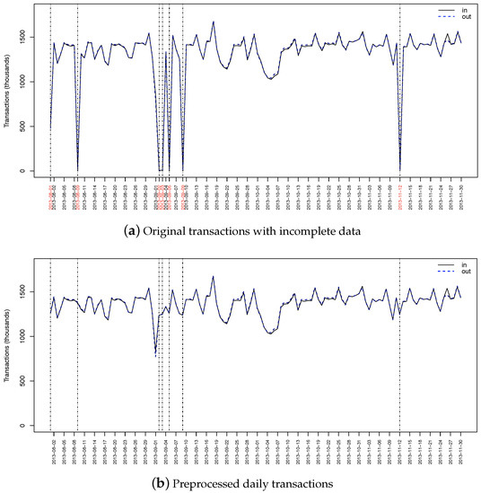
Figure 1.
Aggregated daily transactions in Shenzhen metro smart card data of all transactions over 4-month period, where the black line represents in-station volume, and the dashed blue line denotes out-station volume.
In order to understand the passenger flow at metro stations, we construct Station Flow Data (SFD) from Shenzhen metro smart card data, which reflects streaming tap-in or tap-out passenger flow at stations. We denote hourly tap-in passenger flow data as SFD-in and hourly tap-out flow as SFD-out. Both SFD-in and SFD-out have 118 rows (stations) and 2928 columns (122 days*24 h). For each SFD-in or SFD-out, , , the assignment of is denoted as , meaning which cluster belongs to. Therefore, the objective is to discover accurate partitions for stations.
Each data point in SFD matrix is normalized as
where denotes the passenger volume at h-th time slot of station s, means the vector of stations, and is the normalized value within range .
3.3. Multiple Clusterings Issue
In this section, taking K-means algorithm [46] for example, we illustrate multiple clusterings issue through two observations as follows.
Observation 1.
The optimal number of clusters K might not be unique due to different methods.
For example in Figure 2, when different methods are considered to determine optimal K for SFD-out data, we might have multiple optimal Ks as 2, 3 or 4. Thus, we have three different clusterings as shown in Figure 3.
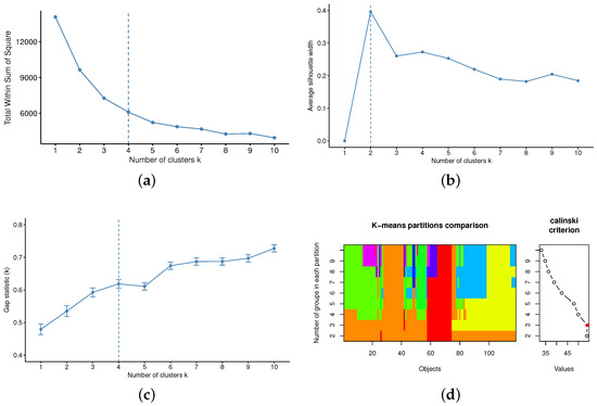
Figure 2.
Determine optimal K with different methods for SFD-out data, which shows that optimal number of clusters depends on the clustering algorithms and metrics. (a) Elbow method [46]: ; (b) Silhouette method [47]: ; (c) Gap statistic method [48]: ; (d) Calinski criterion [49]: .
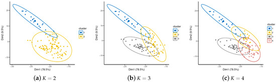
Figure 3.
K-means clustering on SFD-out data, when K takes different optimal values. Cluster plot is visualized using the factoextra package in R, where X-axis and Y-axis represent principal axes and their variable contributions.
Observation 2.
Evaluation of best clustering depends on what measures are considered.
Generally, there are three categories of measures to validate clustering results: (1) internal measures evaluate compactness, connectedness and separation among partitions within each clusterer, such as silhouette coefficient [50] and Dunn index [51]; (2) external measures compute similarity between different clusterings (when alternative clustering is provided), such as Rand index [52], Fowlkes–Mallows index [53], Jaccard index [54] and variation of information [55]; and (3) stability measures evaluate the consistency of clustering by comparing clusterings based on full data set and removal of specific column [56,57].
Table 3 demonstrates clustering performance validation with optimal using SFD-out data, where ↑ denotes larger is better while ↓ means smaller is better, and better clusterings are highlighted by stars. Specifically packages clValid [58], fpc [59] and NbClust [60] in R are employed for computing each measure. We observe that for Silhouette and DI, clusterer performs best; for ARI, FM and Jaccard index, clusterer outperforms others; for VI measure, clusterer stands out; in addition, depending on which stability measure is considered, any one of the three clusterers could be the best.
Table 3.
Clustering validation of K-means with using SFD-out data.
4. Clustering Refinement Framework
To this end, we propose a clustering refinement framework to ensemble isomorphic or heterogeneous clusterers. The intuitions behind are: (1) despite optimal K and parameter settings, it is not guaranteed that current clusterer is the best solution owing to various validation measures; and accordingly (2) clustering refinement—integrating clusterings from multiple clusterers with optimal K by some means— produces better solution. A proposed refinement approach is conducted through ensembling clusterers produced by optimal or near-optimal K settings and stable clustering algorithms, which thus effectively identifies more separative and cohesive partitions of data, and meanwhile is capable of outlier detection.
As a preliminary to our solution, we introduce the concept of cluster member based stability to illustrate instability issue across multiple clustering solutions.
4.1. Cluster Member Based Stability
As discussed in [2], the quality of clustering results can be evaluated through stability; and clustering instability comes from two kinds of random components: (1) different perturbations of data, such as data set sampling; and (2) different initialization and parameter settings of the algorithm.
However, consider exactly the same D with no data perturbations (i.e., data randomness excluded), stable clustering solutions are not yet unique when: (1) multiple Ks are produced when different criteria are used to determine optimal number of clusters; or (2) various measures are evaluated as indicators during clustering algorithm execution. Therefore, we define unstable members as individuals with inconsistent cluster labels across multiple clusterings.
Definition 1
(Unstable member). Suppose there exist two distinct clusterings , individual satisfying is called an unstable member.
As discussed before, instability issue across multiple clusterings remains due to: (1) non-unique optimal K, and (2) difficult-to-determine parameters. Take Figure 3 for example. Since our dataset is high-dimensional, cluster plots are drawn by first two principle components after Principal Component Analysis (PCA) for visualization purpose. For each individual optimal K, in order to eliminate the unstability caused by initialization conditions, we use set.seed() to ensure the repeatability of results, and nstart=50 to generate multiple initial configurations, and thus the best and stable results are reported by each clusterer. We can observe that cluster members in Cluster 1 remain stable in Figure 3a–c; however, when we increase K, members in Cluster 2 in Figure 3a partially shift to Cluster 3 in Figure 3b and later Cluster 4 in Figure 3c. Individuals with multiple cluster labels across different clusterings are unstable members, caused by non-unique optimal K in this scenario.
Another cause of instability issue is input parameters, which is hard to choose because of lack of established argumentation or too expensive computation, especially for some clustering algorithms especially high-dimensional algorithms. Take projected subspace clustering algorithm ProClus [61] for example. Here we use PCA to heuristically determine average cluster dimensionality L. As in Figure 4, is selected by the elbow point in the percentage of variances explained by each principal component; and are considered according to cumulative percentage of variances explained by principal components.
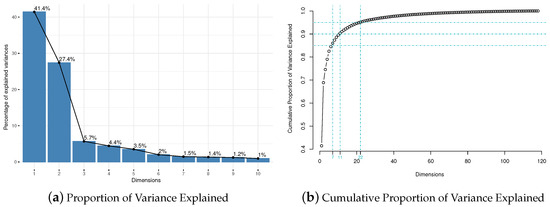
Figure 4.
Illustration of difficult-to-determine parameters. Heuristically choose L by: (a) elbow point in the percentage of variances explained by each principal component; (b) cumulative percentage of variances explained by principal components, i.e., .
Figure 5 demonstrates member based stability with ProClus clustering with different L using the subspace (https://cran.r-project.org/web/packages/subspace) package. For the sake of visualization and understanding, we define station IDs as follows: (1) non-transfer stations are composed of three digits, where the first digit denotes the line number, and the other two digits denote the sequential number of station; (2) transfer stations begin with t followed by three digits, where the first two digits denote intersected two lines, and the last digit means the sequential number of intersections between them. For example, 317 means the 17th station of Line 3, and t122 means the transfer station is the second intersection of Lines 1 and 2.
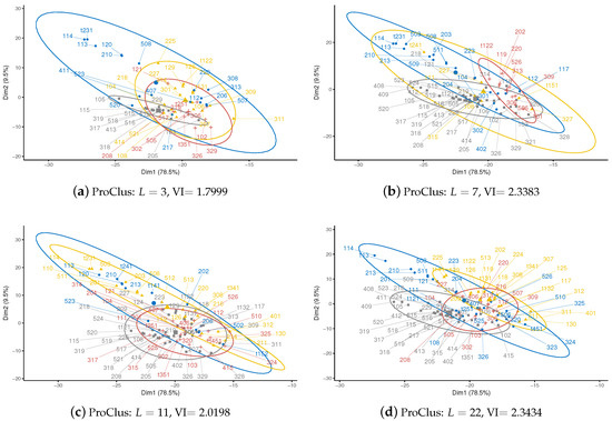
Figure 5.
ProClus clustering on SFD-out data when , where cluster notations are consistent with Figure 3, non-overlapping labels denote station IDs, and VI is measured by comparison with alternative clustering produced by K-means () clusterer. Cluster plot is visualized using the factoextra package in R.
As suggested in Figure 5, owing to difficult-to-determine parameters, which might be determined by some heuristic methods, member relationship between individuals (i.e., stations) and clusters could be unstable. For example, stations 317, 318, 319 are within the same cluster in Figure 5a,b,d, except that 317 shifts to another cluster in Figure 5c. That is, 318 and 319 are of the same group among four ProClus clusterers, while 317 is an unstable member. Note that ProClus detects outliers, which are not classified as objects in clustering results, and thus not shown in the figures accordingly.
However, members with different cluster labels could be still organized within the same cluster, while is the result of unaligned clustering vectors generated by different clusterers. Therefore, we introduce corrected unstable member to illustrate clustering alignment issue.
Definition 2
(Corrected unstable member). Suppose there exist two distinct stable clusterings (). Given individual , its cluster labels in two clusterings are and , and the corresponding cluster centroids are respectively. If , then is corrected unstable member.
Take model-based high-dimensional clustering algorithm HDDC [62] for example. As illustrated in Figure 6, Expectation-Maximisation (EM), Classification E-M (CEM) and Stochastic E-M (SEM) algorithms for model selection with BIC (Bayesian Information Criterion) or ICL (Integrated Complete-data Likelihood) criteria are employed respectively for HDDC clustering [63] using the HDclassif (https://cran.r-project.org/web/packages/HDclassif) package. All three clusterers report five clusters with various cluster labels, reflected as annotation of points in figures. However, it could be easily observed that the clusterings are identical except for notations, and therefore these three clusterings are regarded as the same solution. In fact, cluster labels are already aligned for previous visualization in Figure 3 and Figure 5. From now on, we refer to unstable members as Definition 2.
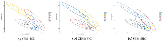
Figure 6.
Illustration of clustering alignment issue: HDDC clusterings on SFD-out data with EM, CEM or SEM models using either ICL or BIC report identical clusters. Cluster plot is visualized using the factoextra package in R.
4.2. Clustering Refinement with Member Based Stability
As discussed before, isomorphic or heterogeneous clusterers could generate multiple stable clusterings, and it is difficult to confirm the best clustering due to various validation measures. In addition, some individuals keep the same membership among multiple clusterings, while unstable members shift across clusters during multiple clusterers. To this end, we propose a clustering refinement procedure based on unstable members to integrate multiple stable clusterings produced by isomorphic or heterogeneous clusterers.
The proposed clustering refinement is illustrated in Algorithm 1. As mentioned before, input clusterer M is supposed to be relatively stable in its own nature. That is, input parameters are carefully selected using existing effective or heuristic methods. The intuition is that in most circumstances there are multiple good clustering solutions available, and each of them could be outstanding from different perspectives. Thus, we ensemble multiple sufficiently good clusterings for refinement.
Suppose we have a set of models with proper parameter settings to ensemble, and a candidate list of potential optimal K determined by various methods (Figure 2). Basically, there are three steps in clustering refinement framework.
Step 1. Initialization clusters by running qualified clusterer with . Since we would align cluster labels as sequentially, minimum K clusterer is first executed to produce minimum number of clusters for the purpose of clustering vector alignment later.
Step 2. Run other clusterers with remaining candidate K, and relabel members by clustering vector alignment. Parameter settings should be carefully chosen to reduce running time; however, details about how to choose parameters for specific clustering algorithm are not considered in the framework. Moreover, clustering vector alignment guarantees cluster labels produced by all clusterers are consistent.
| Algorithm 1: Clustering refinement procedure. |
 |
Figure 7 illustrates the principle of clustering vector alignment. Suppose initially we have two clusters as in Figure 7a, centroids are and respectively, and object belongs to Cluster 1, while belongs to Cluster 2. Later, clusterings Figure 7b,c are produced when using alternative K, and all subsequent clusterings are relabeled according to Figure 7a by nearest centroid. For example, suppose originally belongs to Cluster 2 in upper Figure 7b. Among three centroids, is closest to , so the cluster in which is located (Cluster 2) is relabeled as 1 (Cluster 1) and thus has label 1. Similarly, if originally belongs to Cluster 1 in upper Figure 7b, compared to existing in Figure 7a, is more close to , and thus a new label (Cluster 3) is assigned to the cluster in which is located (Cluster 1), as illustrated in lower Figure 7b. Later on, when a larger K is applied, members closest to newly generated centroid are assigned to greater label. For instance, in clustering Figure 7c, the cluster in which is located is relabeled as Cluster 4 because is the nearest centroid. In this way, we reconstruct clustering vectors by consistently labeling without changing clustering partitions.
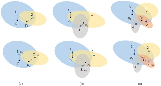
Figure 7.
Illustration of clustering vector alignment process, where denote centroids of clusters with different point annotations, are two example objects, and dashed lines denote distances between and . The upper figures are original clustering labels of (a) , (b) , and (c) , while the lower figures are relabeled clusterings.
Step 3. Make decisions about final cluster labels for all members. We use voting strategies for clustering integration.
- Majority rule: if there is a single label with more than a third of the votes, regard it as the final label directly. Here we use 1/3 instead of 1/2 to eliminate the randomness error in clustering vector alignment. For instance, some clusterers assign NA for detected outliers.
- If there exist multiple majority labels, that means objects are shifting back and forth between clusters, and therefore those packaged unstable members are assigned to a new cluster, determined by their shifting range.
- Otherwise, object occurrences in clusters are random. That is, each time we apply an alternative clusterer, its assignment changes correspondingly. Indeed, random assignment among all clusterers is probably outliers.
For example, suppose , and the clustering vectors are:
For each individual , count the vote of each label among all clusterers in the format of as following:
If vote , majority rule is applied. However, for , the majorities are not unique, and they frequently shift between Clusters 1 and 2. The reason behind could be that the role of is fuzzy between Clusters 1 and 2, and in order to differentiate them from explicit stable members, we assign new labels. Otherwise, if no majority exists, such as , an outlier is detected since it does not belong to any clusters explicitly. Therefore, the final clustering vector is . In this way, clustering results are refined by integrating good enough results from multiple established clusterers.
5. Clustering Results
In this section, we conduct experiments using proposed clustering refinement framework on SFD data. The input settings of Algorithm 1 are described as follows: (1) SFD-out and SFD-in data; (2) K-means, ProClus and HDDC clustering algorithms; (3) Optimal Ks for SFD-out data are , as suggested in Figure 2 and Figure 6; similarly, optimal K for SFD-in data is determined as by WSS, Silhouette, Gap statistics, Calinski criterion respectively; (4) Maximum number of iterations as 100.
The agglomeration property drawn from out-station passenger flow reflects human mobility destination, and the clustering in the light of in-station passenger flow reveals where people come from. According to execution results of Algorithm 1, Figure 8 shows final clustering results over both out-station and in-station passenger flows, from which five clusters of stations are detected. Basically, the final cluster labels are generated by consolidating the overlaps between in-station and out-station clusterings, while the inconsistent parts contribute to outliers. For the convenience of narration, we highlight each cluster from Figure 8a–e.
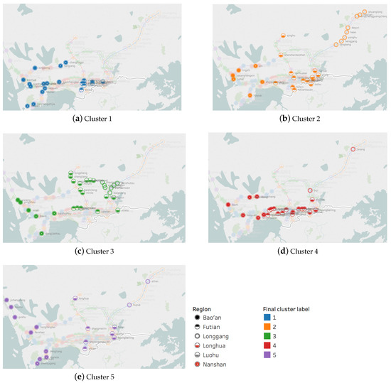
Figure 8.
Map-based visualization of station clusters. The marks are labeled by station names, shape shows details about administrative region, and color of stations shows final cluster labels produced by proposed method. The maps are plotted using Tableau Desktop.
Now we explore the implications of clustering results in Figure 8 with reference to government policy and regulatory documents (http://www.sz.gov.cn/cn/xxgk/zfxxgj/ghjh/), such as “Shenzhen City Master Plan”, “Shenzhen City Land Utilization Master Plan” and “Urban Construction and Land Use in Shenzhen for the Thirteenth Five-year Plan”.
Cluster 1: Strategic development core area—highlighted as blue in Figure 8a. Specifically, stations in Cluster 1 are located in: (1) Baoan central area for high-tech industry operations, research and development headquarters, business services, and cultural and creative industries, such as Baohua (Baohua Station) and Xingdong (Xingdong Station); (2) high-tech zone north district for emerging and future industries, such as Shenda (Shenzhen University Station) and Gaoxinyuan (Hi-Tech Park Station); (3) city government resident areas, such as Shiminzhongxin (Civic Center Station) and Huizhanzhongxin (Convention & Exhibition Center Station).
Cluster 2: Suburb area and transportation junctions—highlighted as orange in Figure 8b. Generally, Cluster 2 is distributed in suburb area, such as teleneurons of each line, and interfaces to other transit modes (i.e., airport, train and checkpoint), such as Shenzhenbeizhan (Shenzhen North Station), Luohu (Luohu Station) and Futiankouan (Futian Checkpoint Station). However, exceptions include: (1) Metro Airport Area, i.e., Jichangdong (Airport East Station), Houri (Hourui Station) and Gushu (Gushu Station); (2) Qianhai Shekou Free Trade Zone, including Chiwan (Chiwan Station), Shekougang (Shekou Port Station) and Haishangshijie (Sea World Station); (3) Ban Xue Gang Tech area, such as Longhua (Longhua Station) and Longsheng (Longsheng Station); (4) Shenzhen airport Longgang terminal, i.e., Ailian (Ailian Station).
Cluster 3: Technology and industrial development area—highlighted as green in Figure 8c. Specifically, regions around Cluster 3 are: (1) Ban Xue Gang Tech area for new generation of information industry such as high-end software and intelligent terminal, such as Longsheng (Longsheng Station) and Shangtang (Shangtang Station); (2) Shenzhen North Station business center area for commercial business, e-commerce and service industry, such as Minzhi (Minzhi Station) and Baishilong (Baishilong Station); (3) Luohu Sungang-Qingshuihe district, primarily for commercial commerce, cultural and creative industries, such as Caopu (Caopu Station).
Cluster 4: Futian-Luohu economic center—highlighted as red in Figure 8d, serving as the axis of the urban economy, such as Guomao (Guomao Station) and Chegongmiao (Chegongmiao Station). Note that Chegongmiao was a non-transfer station in 2013; however, as the center at Futian-Luohu economic center as well as one of the key development areas in Thirteenth Five-year Plan of Shenzhen, Chegongmiao becomes the first transfer hub of four lines in Shenzhen afterwards.
Cluster 5: Ambiguous functional stations—highlighted as purple in Figure 8e. To be specific, they are: (1) suburb but key development area, such as exceptions mentioned in Type II; (2) Meilin-Caitian district, a key area within Meilin industrial zone in the north of Futian, which is a newly qualified key development area in the Thirteenth Five-Year Plan of Shenzhen, i.e., Shangmeilin (Shangmeilin Station); (3) intermediate region nearby or between development areas, such as Honglangbei (Honglang North Station) nearby high-tech zone north district. Indeed, this type of stations are generated by unstable members randomly shifting among multiple clusterings for both SFD-out and SFD-in. We have 19 outlier stations detected as listed in Table 4.
Table 4.
Outlier stations of Cluster 5.
Moreover, Figure 9 demonstrates temporal patterns in terms of in-station and out-station passenger volume for each type of stations using typical examples. From the perspective of commuting behavior, temporal pattern of passengers can be explained in the following.
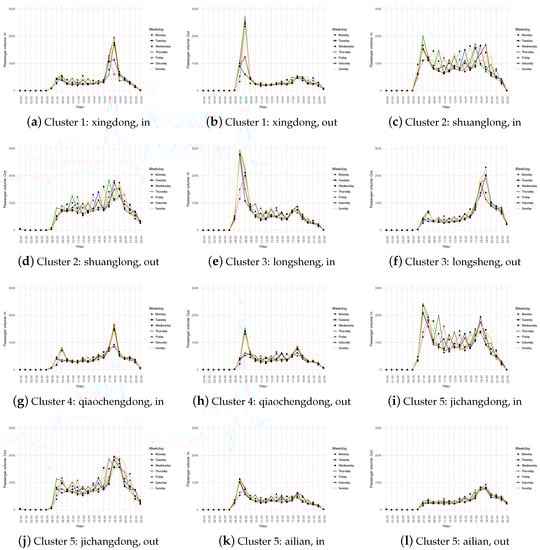
Figure 9.
Hourly passenger volume in terms of in-station and out-station by weekdays for example stations in Type I, II, III, IV, V.
- Cluster 1 in Figure 9a,b: morning peak only shows in out-station flow around 08:00, while evening peak only appears in in-station flow around 18:00, indicating Xingdong station might be workplace and people commute regularly to and from work. That is, people traveling at Cluster 1 stations are likely to be commuters.
- Cluster 2 in Figure 9c,d: no significant peak appears during the whole day period. Therefore, passengers at Cluster 2 stations probably exhibit random behavior.
- Cluster 3 in Figure 9e,f: morning peak only shows in in-station flow around 07:00, while evening peak only appears in out-station flow around 19:00, indicating Longsheng might be place of residence. Corresponding to Figure 9a,b, people travel from residence at 07:00 to workplace at 08:00, and return from work at 18:00 to home at 19:00. Therefore, we infer that passengers at residential stations are exactly the same with those appear at workplace stations. That is, passengers at Cluster 3 stations are also regular commuters.
- Cluster 4 in Figure 9g,h: both in-station and out-station have morning peaks and evening peaks. Specifically, the in-station morning peak is lower than in-station evening peak, and out-station shows the opposite pattern. Besides, the peak volumes are lower compared to Clusters 1 and 3. Hence, we speculate the function of Cluster 4 stations falls in between labor-intensive and densely settled area. However, the significant peak characteristics indicate commuters as well despite land use functionality.
- Cluster 5 in Figure 9i–l: temporal pattern of Cluster 5 is not that random as Cluster 2, as shown in Figure 9i,j; and meanwhile does not significantly follow the morning and evening peak laws as Clusters 1,3,4, as shown in Figure 9k,l. Therefore, passengers at Cluster 5 stations are neither random nor typical commuters; nevertheless, the traffic pattern basically follows the law of morning-evening traveling in daily life.
In order to further understand spatial aggregation of subway stations, we additionally introduce external environmental factors by collecting population size and POI counts from Baidu Map service (http://lbsyun.baidu.com) for each individual subway station. POI based variables include the number of hospitals, restaurants, residential units, working units, hotels, shopping centers, schools, banks and bus stops. Note that each variable is obtained by the number of POIs within 500-meter area [64] around each station.
Moran’s I [65] is a widely used statistic indicator for measuring spatial autocorrelation. In Table 5, Moran’s I Index value and associated z-value and p-value are calculated to evaluate the significance of spatial autocorrelation, and all statistics are computed in GeoDa [66]. In general, Moran’s I ranges from −1 to +1; positive Moran’s I close to +1 indicates clustering and negative Moran’s I value near −1 indicates dispersion. Z-value measures standard deviation, and p-value represents significant level. Basically when performing Moran’s I test, small p-value and a very high (or a very low, negative) z-value indicate observed pattern is unlikely to exhibit theoretical randomness pattern represented by null hypothesis.
Table 5.
Spatial autocorrelation analysis results of environmental variables.
In Table 5, Moran’s I is calculated as global univariate indicator, and adjusted Moran’s I is calculated as Anselin’s local Moran’s I test with Empirical Bayesian (EB) rate [67] when clustering pattern of subway stations is considered. The significance test is computed by 999 permutations. We observe that Moran’s I values of all variables are positive and could be up to 0.7638 (population), which means that environmental factors are spatially autocorrelated with highly significant confidence level (>99%). Moreover, adjusted Moran’s I turns to be close to global Moran’s I, which suggests the clustering pattern of subway stations is consistent with spatial autocorrelation of environmental factors of urban city.
Besides, regression analysis is performed to reconfirm the spatial dependence. As shown in Table 6, after classical Ordinary Least Square (OLS) regression, Moran’s I is highly significant (0.00002), indicating strong spatial autocorrelation of the residuals. The significant test results for spatial dependence in linear models are: LM-error (0.00775) ≻ Robust LM-error (0.01966) ≻ LM-lag (0.03238) ≻ Robust LM-lag (0.08694). Thus, regression with spatial error LM-error model is employed to deduce the correlation coefficients of all variables, as listed in the lower section in Table 5. Due to data integrity issues and the inconsistency in timespan (passenger flow data was collected in 2013 while POI data is obtained in 2018), the correlation coefficients between POI counts and clusters are not highly significant (<0.5). However, still, we can see that hospital (0.4646), hotel (0.3972) and bus stop (0.3661) are more positively correlated with the clustering pattern of subway stations, while school (−0.4447) and residential (−0.3882) are more negatively correlated.
Table 6.
Diagnostics for spatial dependence.
6. Conclusions
In this study, we utilized cluster analysis approach to reveal functional spatial structure embedded in subway stations using smart card data collected through AFC systems. Specifically, we developed a clustering refinement framework by introducing the concept of cluster member stability and investigating member shifting patterns across isomorphic or heterogeneous clusterers. Furthermore, the intrinsic connection between public transit and urban spatial structure was validated with references to urban government planning policies and strategies through a case study of Shenzhen city.
In this paper we demonstrate that urban spatial structure could be concealed in public transit smart card data clustering with no additional information required. However, we do not probe into the interaction details between public transit and urban spatial structure, because it is a complex issue which involves many factors and needs to be verified by historical evolution. Instead, based on the smart card data of Shenzhen Metro, urban spatial structure is conceptualized as geographical layout in urban planning orientation and land development policies, and implication of five clusters is explained through spatial overlapping between surrounding area of subway stations and urban layout. Moreover, to further understand the effectiveness of clustering results, we explore the spatial correlation between POI based environmental factors and subway clusters using Moran’s I statistics and spatial regression analysis. Consequently, the conclusion could be drawn that clustering pattern of subway stations is consistent with spatial autocorrelation of environmental factors of urban city.
In practice the clustering structure of subway stations could be one of the significant decision-making references for urban planning, land utilization planning and rail transit construction planning. Take Chegongmiao station as an example, in 2013 subway clusterings, Chegongmiao station is found to be located at Cluster 4 (Futian-Luohu economic center). Furthermore, Chegongmiao area is identified as one of the key development zones in Thirteenth Five-Year Plan of Shenzhen. Accordingly, Chegongmiao becomes the first transfer station of four lines in Shenzhen afterwards in 2016. Thus it can be inferred that according to subway clusterings and urban planning policies, considering surrounding properties of subway stations, rail transit lines could be extended and stations could become transfer hubs. In fact, as indicated by the spatial correlation between environmental factors and subway stations, the hidden aggregation pattern in public transit stations could be useful for expansion, optimization and construction of public infrastructure, hospital, industrial, entertainment, commercial, and transportation, etc.
In future works, we would like to extensively examine experimental comparison among different clustering algorithms with proposed ensemble refinement method; and further explore public transit data combined with fine-grained individual mobility data such as bicycles, taxis or mobile phone trajectories to capture a more elaborated picture of urban spatial structure. Besides, application oriented decision-making support on urban space management will be further investigated.
Author Contributions
Conceptualization, L.T. and Y.Z.; methodology, L.T. and Y.Z.; data analysis, L.T.; validation, L.T. and Y.H.; writing, original draft preparation, L.T.; writing, review and editing, L.T., Y.Z., K.L.T. and L.P.; supervision, K.L.T. All authors have read and agreed to the published version of the manuscript.
Funding
This research work was partly supported by National Key Research and Development Program of China (Grant No. 2016YFC0800100), National Natural Science Foundation of China (Grant No. 71901188), and the Research Grants Council Theme-based Research Scheme (Grant No. T32-101/15-R).
Conflicts of Interest
The authors declare no conflict of interest.
References
- Dittmar, H.; Ohland, G. The New Transit Town: Best Practices in Transit-Oriented Development; Island Press: Washington, DC, USA, 2004. [Google Scholar]
- Von Luxburg, U. Clustering stability: An overview. Found. Trends Mach. Learn. 2010, 2, 235–274. [Google Scholar]
- Strehl, A.; Ghosh, J. Cluster ensembles—A knowledge reuse framework for combining multiple partitions. J. Mach. Learn. Res. 2002, 3, 583–617. [Google Scholar]
- Suzuki, H.; Cervero, R.; Iuchi, K. Transforming Cities with Transit: Transit and Land-Use Integration for Sustainable Urban Development; World Bank: Washington, DC, USA, 2013. [Google Scholar]
- Murray, A.T. A Coverage Model for Improving Public Transit System Accessibility and Expanding Access. Ann. Oper. Res. 2003, 123, 143–156. [Google Scholar] [CrossRef]
- Daniels, R.; Mulley, C. Explaining walking distance to public transport: The dominance of public transport supply. J. Transp. Land Use 2013, 6, 5–20. [Google Scholar] [CrossRef]
- Guo, Q.; Dian-Tin, W.U.; Bao, J. Evaluation of Accessibility in Urban Rail Transit Network of Beijing Based on Transfer Efficiency Index and the Analyze of Its Cause. Econ. Geogr. 2012, 32, 38–44. [Google Scholar]
- Papa, E.; Bertolini, L. Accessibility and Transit-Oriented Development in European metropolitan areas. J. Transp. Geogr. 2015, 47, 70–83. [Google Scholar] [CrossRef]
- Kim, S.; Ulfarsson, G.F.; Hennessy, J.T. Analysis of light rail rider travel behavior: Impacts of individual, built environment, and crime characteristics on transit access. Transp. Res. Part Policy Pract. 2007, 41, 511–522. [Google Scholar] [CrossRef]
- Cheng, Y.H.; Chen, S.Y. Perceived accessibility, mobility, and connectivity of public transportation systems. Transp. Res. Part 2015, 77, 386–403. [Google Scholar] [CrossRef]
- Zhang, Y.; Martens, K.; Long, Y. Revealing group travel behavior patterns with public transit smart card data. Travel Behav. Soc. 2018, 10, 42–52. [Google Scholar] [CrossRef]
- Zhao, L.; Shen, L. The impacts of rail transit on future urban land use development: A case study in Wuhan, China. Transp. Policy 2018, 81, 396–405. [Google Scholar] [CrossRef]
- Bowes, D.R.; Ihlanfeldt, K.R. Identifying the Impacts of Rail Transit Stations on Residential Property Values. J. Urban Econ. 2001, 50, 1–25. [Google Scholar] [CrossRef]
- Du, H.; Mulley, C. The short-term land value impacts of urban rail transit: Quantitative evidence from Sunderland, UK. Land Use Policy 2007, 24, 223–233. [Google Scholar] [CrossRef]
- Xiaohui, L.E.; Chen, J.; Yang, J. Impact of rail transit on urban spatial structure in Shenzhen: Analysis based on land parcel price and FAR gradients. Geogr. Res. 2016, 11, 2091–2104. [Google Scholar]
- Long, Y.; Sun, L.; Tao, S.; Laboratory, F.C. A Review of Urban Studies Based on Transit Smart Card Data. Urban Plan. Forum 2015, 3, 70–77. [Google Scholar]
- Pelletier, M.; Trepanier, M.; Morency, C. Smart card data use in public transit: A literature review. Transp. Res. Part -Emerg. Technol. 2011, 19, 557–568. [Google Scholar] [CrossRef]
- Nassir, N.; Hickman, M.; Ma, Z.L. Activity detection and transfer identification for public transit fare card data. Transportation 2015, 42, 683–705. [Google Scholar] [CrossRef]
- Bauer, D.; Richter, G.; Asamer, J.; Heilmann, B.; Lenz, G.; Kölbl, R. Quasi-Dynamic Estimation of OD Flows From Traffic Counts Without Prior OD Matrix. IEEE Trans. Intell. Transp. Syst. 2018, 19, 2025–2034. [Google Scholar] [CrossRef]
- Munizaga, M.A.; Palma, C. Estimation of a disaggregate multimodal public transport Origin-Destination matrix from passive smartcard data from Santiago, Chile. Transp. Res. Part C 2012, 24, 9–18. [Google Scholar] [CrossRef]
- Utsunomiya, M.; Attanucci, J.; Wilson, N.H.M. Potential uses of transit smart card registration and transaction data to improve transit planning. Transp. Res. Rec. 2006, 1971, 119–126. [Google Scholar] [CrossRef]
- Wang, Z.J.; Li, X.H.; Chen, F. Impact evaluation of a mass transit fare change on demand and revenue utilizing smart card data. Transp. Res. Part Policy Pract. 2015, 77, 213–224. [Google Scholar] [CrossRef]
- Zhao, J.; Frumin, M.; Wilson, N.; Zhao, Z. Unified estimator for excess journey time under heterogeneous passenger incidence behavior using smartcard data. Transp. Res. Board Meet. 2013, 34, 70–88. [Google Scholar] [CrossRef]
- Hao, J.; Zhu, J.; Zhong, R. The rise of big data on urban studies and planning practices in China: Review and open research issues. J. Urban Manag. 2015, 4, 92–124. [Google Scholar] [CrossRef]
- Bagchi, M.; White, P.R. The potential of public transport smart card data. Transport Policy 2005, 12, 464–474. [Google Scholar] [CrossRef]
- Ma, X.; Wu, Y.J.; Wang, Y.; Chen, F.; Liu, J. Mining smart card data for transit riders travel patterns. Transp. Res. Part -Emerg. Technol. 2013, 36, 1–12. [Google Scholar] [CrossRef]
- Munizaga, M.; Devillaine, F.; Navarrete, C.; Silva, D. Validating travel behavior estimated from smartcard data. Transp. Res. Part 2014, 44, 70–79. [Google Scholar] [CrossRef]
- Zhao, J.; Zhang, F.; Tu, L.; Xu, C.; Shen, D.; Tian, C.; Li, X.Y.; Li, Z. Estimation of passenger route choice pattern using smart card data for complex metro systems. IEEE Trans. Intell. Transp. Syst. 2017, 18, 790–801. [Google Scholar] [CrossRef]
- Yang, Y.; Tian, L.; Yeh, A.G.O.; Li, Q.Q. Zooming into individuals to understand the collective: A review of trajectory-based travel behaviour studies. Travel Behav. Soc. 2014, 1, 69–78. [Google Scholar]
- Zhong, C.; Arisona, S.M.; Huang, X.; Batty, M.; Schmitt, G. Detecting the dynamics of urban structure through spatial network analysis. Int. J. Geogr. Inf. Sci. 2014, 28, 2178–2199. [Google Scholar] [CrossRef]
- Roth, C.; Kang, S.M.; Batty, M.; Barthelemy, M. Structure of Urban Movements: Polycentric Activity and Entangled Hierarchical Flows. PLoS ONE 2011, 6, e15923. [Google Scholar] [CrossRef]
- Long, Y.; Shen, Z. Discovering functional zones using bus smart card data and points of interest in Beijing. In Geospatial Analysis to Support Urban Planning in Beijing; Springer: Berlin/Heidelberg, Germany, 2015; pp. 193–217. [Google Scholar]
- Ma, X.; Liu, C.; Wen, H.; Wang, Y.; Wu, Y.J. Understanding commuting patterns using transit smart card data. J. Transp. Geogr. 2017, 58, 135–145. [Google Scholar] [CrossRef]
- Zhong, C.; Arisona, S.M.; Huang, X.; Schmitt, G. Identifying Spatial Structure of Urban Functional Centers Using Travel Survey Data: A Case Study of Singapore. In Proceedings of the ACM Sigspatial International Workshop on Computational MODELS of Place, Orlando, FL, USA, 5 November 2013; pp. 28–33. [Google Scholar]
- Long, Y.; Thill, J.C. Combining smart card data and household travel survey to analyze jobs-housing relationships in Beijing. Comput. Environ. Urban Syst. 2015, 53, 19–35. [Google Scholar] [CrossRef]
- Zhong, C.; Schlapfer, M.; Arisona, S.M.; Batty, M.; Ratti, C.; Schmitt, G. Revealing centrality in the spatial structure of cities from human activity patterns. Urban Stud. 2017, 54, 437–455. [Google Scholar] [CrossRef]
- Liu, Y.; Sui, Z.; Kang, C.; Gao, Y. Uncovering Patterns of Inter-Urban Trip and Spatial Interaction from Social Media Check-In Data. PLoS ONE 2014, 9, e86026. [Google Scholar] [CrossRef] [PubMed]
- Xu, R.; Wunsch, D. Survey of clustering algorithms. IEEE Trans. Neural Netw. 2005, 16, 645–678. [Google Scholar] [CrossRef]
- Kaufman, L.; Rousseeuw, P.J. Finding Groups in Data: An Introduction to Cluster Analysis; John Wiley & Sons: Hoboken, NJ, USA, 2009; Volume 344. [Google Scholar]
- Kriegel, H.P.; Kröger, P.; Zimek, A. Clustering high-dimensional data: A survey on subspace clustering, pattern-based clustering, and correlation clustering. ACM Trans. Knowl. Discov. Data 2009, 3, 1. [Google Scholar]
- Vegapons, S.; Ruizshulcloper, J. A survey of clustering ensemble algorithms. Int. J. Pattern Recognit. Artif. Intell. 2011, 25, 337–372. [Google Scholar] [CrossRef]
- Fern, X.Z.; Brodley, C.E. Random projection for high dimensional data clustering: A cluster ensemble approach. In Proceedings of the 20th International Conference on Machine Learning (ICML’03), Washington, DC, USA, 21–24 August 2003; pp. 186–193. [Google Scholar]
- Yang, F.; Li, X.; Li, Q.; Li, T. Exploring the diversity in cluster ensemble generation: Random sampling and random projection. Expert Syst. Appl. 2014, 41, 4844–4866. [Google Scholar] [CrossRef]
- Topchy, A.P.; Law, M.H.; Jain, A.K.; Fred, A.L. Analysis of consensus partition in cluster ensemble. In Proceedings of the Fourth IEEE International Conference on Data Mining, 2004. ICDM’04, Brighton, UK, 1–4 November 2004; pp. 225–232. [Google Scholar]
- Alizadeh, H.; Minaei-Bidgoli, B.; Parvin, H. Cluster ensemble selection based on a new cluster stability measure. Intell. Data Anal. 2014, 18, 389–408. [Google Scholar] [CrossRef]
- Hartigan, J.A.; Wong, M.A. Algorithm AS 136: A k-means clustering algorithm. J. R. Stat. Soc. Ser. (Appl. Stat.) 1979, 28, 100–108. [Google Scholar] [CrossRef]
- Rousseeuw, P.J.; Kaufman, L. Finding Groups in Data; Wiley Online Library Hoboken: Hoboken, NJ, USA, 1990. [Google Scholar]
- Tibshirani, R.; Walther, G.; Hastie, T. Estimating the number of clusters in a data set via the gap statistic. J. R. Stat. Soc. Ser. (Stat. Methodol.) 2001, 63, 411–423. [Google Scholar] [CrossRef]
- Caliński, T.; Harabasz, J. A dendrite method for cluster analysis. Commun.-Stat.-Theory Methods 1974, 3, 1–27. [Google Scholar] [CrossRef]
- Rousseeuw, P.J. Silhouettes: A graphical aid to the interpretation and validation of cluster analysis. J. Comput. Appl. Math. 1987, 20, 53–65. [Google Scholar] [CrossRef]
- Halkidi, M.; Batistakis, Y.; Vazirgiannis, M. On clustering validation techniques. J. Intell. Inf. Syst. 2001, 17, 107–145. [Google Scholar] [CrossRef]
- Rand, W.M. Objective criteria for the evaluation of clustering methods. J. Am. Stat. Assoc. 1971, 66, 846–850. [Google Scholar] [CrossRef]
- Fowlkes, E.B.; Mallows, C.L. A method for comparing two hierarchical clusterings. J. Am. Stat. Assoc. 1983, 78, 553–569. [Google Scholar] [CrossRef]
- Milligan, G.W.; Cooper, M.C. A study of the comparability of external criteria for hierarchical cluster analysis. Multivar. Behav. Res. 1986, 21, 441–458. [Google Scholar] [CrossRef]
- Meilă, M. Comparing clusterings—an information based distance. J. Multivar. Anal. 2007, 98, 873–895. [Google Scholar] [CrossRef]
- Datta, S.; Datta, S. Comparisons and validation of statistical clustering techniques for microarray gene expression data. Bioinformatics 2003, 19, 459–466. [Google Scholar] [CrossRef]
- Yeung, K.Y.; Haynor, D.R.; Ruzzo, W.L. Validating clustering for gene expression data. Bioinformatics 2001, 17, 309–318. [Google Scholar] [CrossRef]
- Brock, G.; Pihur, V.; Datta, S.; Datta, S. clValid, an R package for cluster validation. J. Stat. Softw. 2008, 25, 4. [Google Scholar] [CrossRef]
- Hennig, C. fpc: Flexible procedures for clustering. R Package Version 2010, 2, 3. [Google Scholar]
- Charrad, M.; Ghazzali, N.; Boiteau, V.; Niknafs, A.; Charrad, M.M. Package ‘NbClust’. J. Stat. Soft 2014, 61, 1–36. [Google Scholar]
- Aggarwal, C.C.; Wolf, J.L.; Yu, P.S.; Procopiuc, C.; Park, J.S. Fast algorithms for projected clustering. In Proceedings of the ACM SIGMoD Record, Philadelphia, PA, USA, 1–3 June 1999; ACM: New York, NY, USA, 1999; Volume 28, pp. 61–72. [Google Scholar]
- Bouveyron, C.; Girard, S.; Schmid, C. High-dimensional data clustering. Comput. Stat. Data Anal. 2007, 52, 502–519. [Google Scholar] [CrossRef]
- Bergé, L.; Bouveyron, C.; Girard, S. HDclassif: An R package for model-based clustering and discriminant analysis of high-dimensional data. J. Stat. Softw. 2012, 46, 1–29. [Google Scholar] [CrossRef]
- Kim Dovey, E.P.; Ristic, M. Mapping Urbanities: Morphologies, Flows, Possibilities; Routledge: New York, NY, USA, 2017. [Google Scholar]
- Moran, P.A.P. The Interpretation of Statistical Maps. J. R. Stat. Soc. 1948, 10, 243–251. [Google Scholar] [CrossRef]
- Anselin, L.; Syabri, I.; Kho, Y. GeoDa: An Introduction to Spatial Data Analysis. Geogr. Anal. 2006, 38, 5–22. [Google Scholar] [CrossRef]
- Pui-Jen, T. Application of Moran’s Test with an Empirical Bayesian Rate to Leading Health Care Problems in Taiwan in a 7-Year Period (2002–2008). Glob. J. Health Sci. 2012, 4, 63–77. [Google Scholar]
© 2020 by the authors. Licensee MDPI, Basel, Switzerland. This article is an open access article distributed under the terms and conditions of the Creative Commons Attribution (CC BY) license (http://creativecommons.org/licenses/by/4.0/).