Numerical Study on the Phase Sensitivity Variation in Low Frequency Primary Microphone Calibrations

Abstract

The low frequency phase characteristics of microphones in a monitoring system are crucial for characterizing large-scale natural and artificial activities—e.g., earthquakes, nuclear explosions, or rocket launchings. At present, microphones are simultaneously calibrated using in-situ or calibrator methods to get their phase consistency. However, the essential primary calibration, which traces their phase sensitivity to basic physical quantities, is grossly overlooked. Recently, we speculated that the microphone phase sensitivity is acoustically controlled by the pressure leakage and heat conduction effects in its back chamber, which will vary at low frequencies. Therefore, by means of the FEA (Finite Element Analysis) technique, simulations of laser pistonphone-based primary microphone calibrations are conducted both in the frequency and time domains. The frequency domain simulation quantifies the phase variation, while the time domain analysis helps us to understand the variation mechanism. It is found that the low frequency phase sensitivity is greatly influenced by its geometries and the venting state and should be pre-calibrated before serving.

1. Introduction

In the areas of sound source localization, photo-acoustic imaging, and sound intensity measurement, the phase characteristics of microphones are as important as their modulus characteristics [1,2,3,4]. Nowadays, the study of low-frequency sound and infrasound is developing rapidly, as promoted by the monitoring requirements for a wide variety of large-scale natural and artificial activities—e.g., earthquakes, volcanos, tsunamis, nuclear explosions, supersonic jets, rocket launchings, duct transportation, and industrial production [5,6,7,8]. All the above studies require simultaneous measurement using the microphone monitoring system; by resolving the time differences in acoustic signals from different microphones, the spatial localization and separation are determined. Apparently, the phase characteristics of microphones are key to low-frequency sound and infrasound measurements [9].

The techniques used for calibrating the phase response of the microphone mainly include the in situ method, the loudspeaker or exciter-based calibrator, the wave guide method, the newly proposed pressure gauge comparison method, the reciprocity method, and the laser pistonphone method. The in situ method is widely used to get the phase consistency of microphones in the array [10,11]. However, the calibration results are only applicable to the current system layout. Once the installation position is changed or the microphone is replaced, a recalibration is required. Moreover, due to the free field requirement and the wind noise in the infrasound measurement, the use of the in situ method in the infrasound range is quite limited. When multiple microphones are connected to the loudspeaker or exciter-based calibrator, their phase consistency can be calibrated in the frequency range of 0.01 to 100 Hz [12,13,14,15]. Y.C. Yang of the Institute of Acoustics, Chinese Academy of Sciences, has proposed a calibration system to calibrate the designed infrasound microphone down to 0.001 Hz. The microphones are arranged along a circumference and connected to the sound source by pipes of equal length so that their phase consistency is obtained [16]. More importantly, F. Larsonner et al. studied the phase sensitivities of MB 2005 and MB3 microbarometers in the frequency range of 0.02 to 20 Hz and reported the phase leading phenomenon [15]. The wave guide method and the pressure gauge comparison method require reference sensors to be the comparison standard [17,18]. Depending on that, the calibrating sound pressure in the above methods is obtained experimentally from a reference sensor but not theoretically, and thus these methods all belong to secondary calibration techniques.

The above infrasound calibration studies mainly focus on getting the phase consistency of infrasound sensors based on the comparative (secondary) calibrations, but the primary calibration technique is little studied. The reciprocity method as standardized in IEC (International Electrotechnical Commission) 61094-2 [19] is the most widely accepted primary calibration technique. R. Nel et al. studied the modulus and phase sensitivities of microphones based on the reciprocity method in the frequency range of 1 to 100 Hz and found that the low frequency phase sensitivity is influenced more by the coupler and microphone geometries [20]. R. Jackett et al. determined the phase sensitivity uncertainty and found that the low-frequency uncertainty caused by the pressure leakage effect cannot be ignored [21]. However, due to the great signal attenuation and the model inapplicability, this method is not applicable to the wide infrasound frequency range below 1 Hz.

The laser pistonphone technique is widely used in National Metrology Institutes (NMIs)—e.g., the National Physical Laboratory (NPL), the National Metrology Institute of Turkey (UME), the National Metrology Institute of Japan (NMIJ), the National Institute of Metrology, China (NIM), etc.—as a supplement to the reciprocity method to conduct primary microphone calibrations down to even 0.001 Hz [22,23,24,25]. The laser pistonphone, as shown in Figure 1, produces a sinusoidal sound pressure in the chamber. The time relationship between the calibrating sound pressure and the microphone voltage output is the desired phase sensitivity of the microphone.

For the primary calibration, the calibrating sound pressure in the chamber is given by [25]

$$\underset{\_}{p}=p_L{\underset{\_}{p}}_{\mathrm{lc}}{\underset{\_}{p}}_{\mathrm{hc}}{p}_{\mathrm{wc}},$$

(1)

in which,

$$p_L=\kappa P_0\Delta V/V_0,$$

(2)

$${\underset{\_}{p}}_{lc}=1/\left(1+1/j\omega T_a\right),$$

(3)

$${\underset{\_}{p}}_{\mathrm{hc}}=\left(1+(\kappa -1){\underset{\_}{E}}_{pV}\right)/\kappa ,$$

(4)

where p_L is the lumped pistonphone model, κ is the specific heat ratio, P₀ is the static pressure, △V is the volume variation in the chamber, and V₀ is the chamber volume. p_lc, p_hc, and p_wc are corrections for the pressure leakage, heat conduction, and wave motion effects [20,21,22], in which ω is the angular frequency, T_a is the leakage time constant of the pistonphone, E_pV is its temperature transfer function, and p_wc (wave motion correction) is quite small and can be omitted. It should particularly be noted that the pressure leakage and heat conduction corrections p_lc and p_hc are both complex quantities, which means that the calibrating sound pressure is not synchronized with the piston displacement excitation, and so the phase difference occurs between them.

Let us further analyze the calibration process as shown in Figure 1a. The microphone is essentially a parallel-plate capacitor enclosed by a chamber [26]. When the calibrating sound pressure excites the diaphragm, an associating sound pressure will be generated in the back chamber. This sound pressure will also experience pressure leakage and heat conduction effects [27], and the diaphragm deformation of the microphone is then determined by these two sound pressures and its elasticity. Due to the above amplitude attenuation and phase deviation of the generated sound pressures, the microphone voltage output (equivalent to the diaphragm deformation) will not be synchronized with the calibrating sound pressure, and so its phase sensitivity will vary at low frequencies.

However, the above considerations are only based on qualitative analysis, and the mechanism and characteristics of the variation phenomena are hard to imagine. In this paper, by taking advantage of the FEA (Finite Element Analysis) technique the independent phase responses of sound pressures both in the pistonphone and the microphone are simulated considering the influence of multi-physical factors. The phase sensitivities of the microphone when its vent is connected to the calibrating sound field or the outside atmosphere are obtained based on a proposed joint simulation method. Both frequency and time domain simulations are conducted to quantify the variation value of the phase sensitivity and reveal its variation mechanism. The results verified severe phase sensitivity variations at low frequencies, which are greatly influenced by the microphone geometries and the venting state during calibrations. It is therefore recommended to obtain the primary phase sensitivity of the microphone before serving.

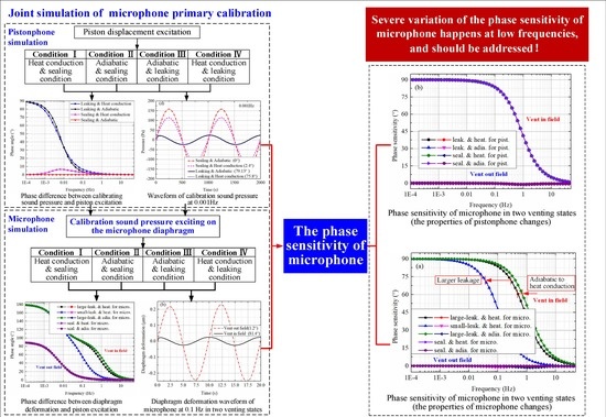
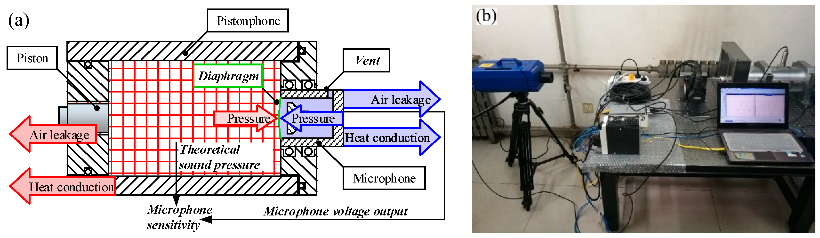
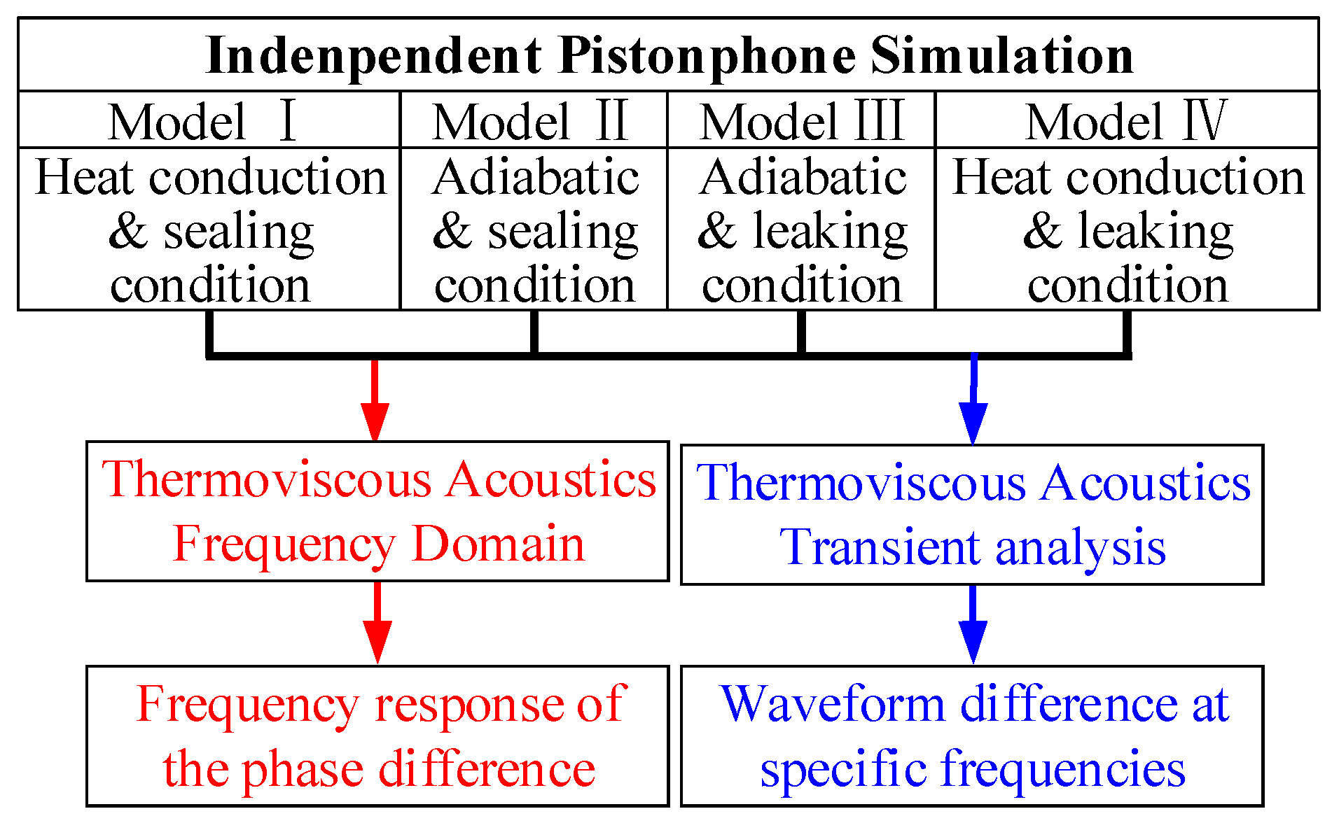
2. Independent Pistonphone Simulation

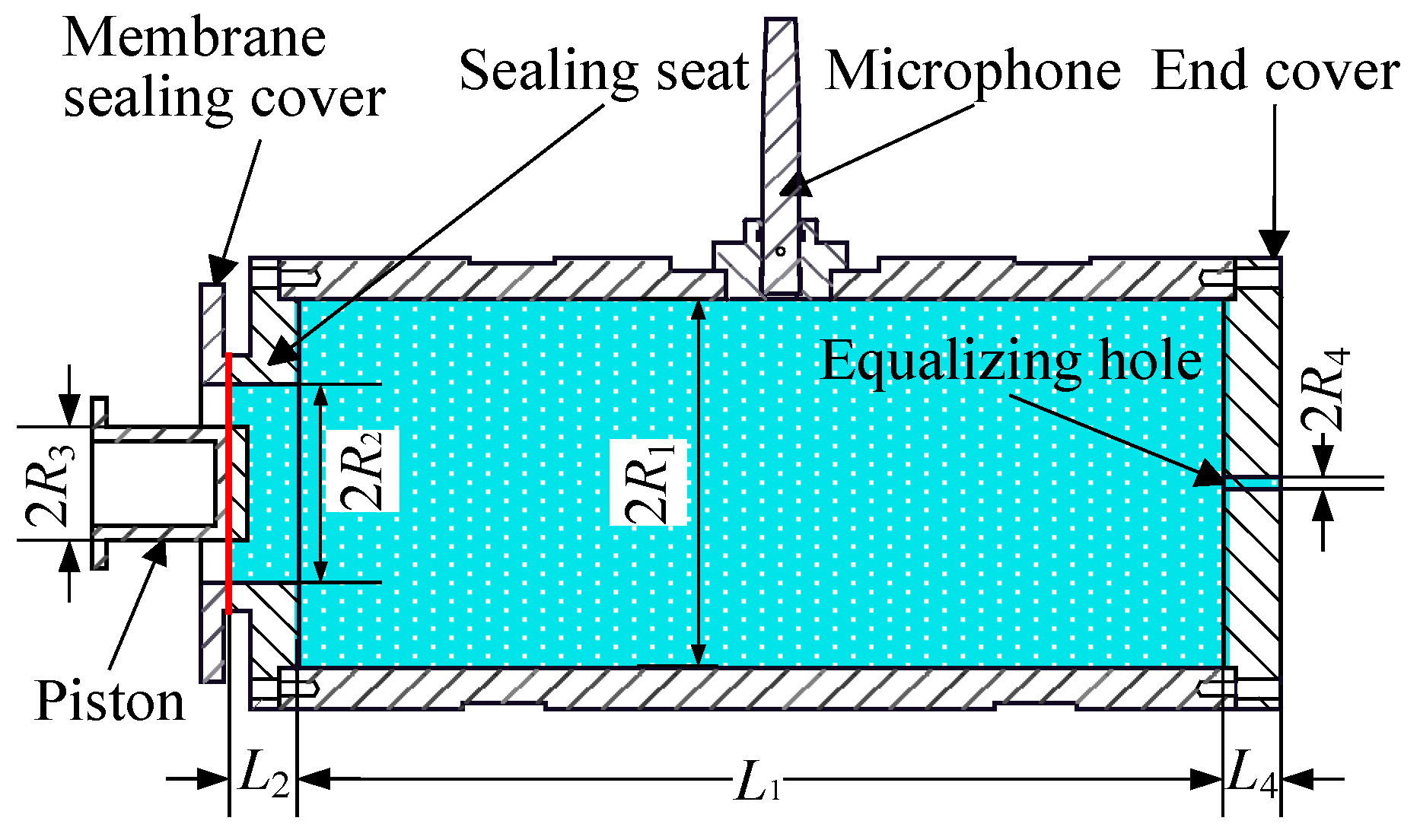
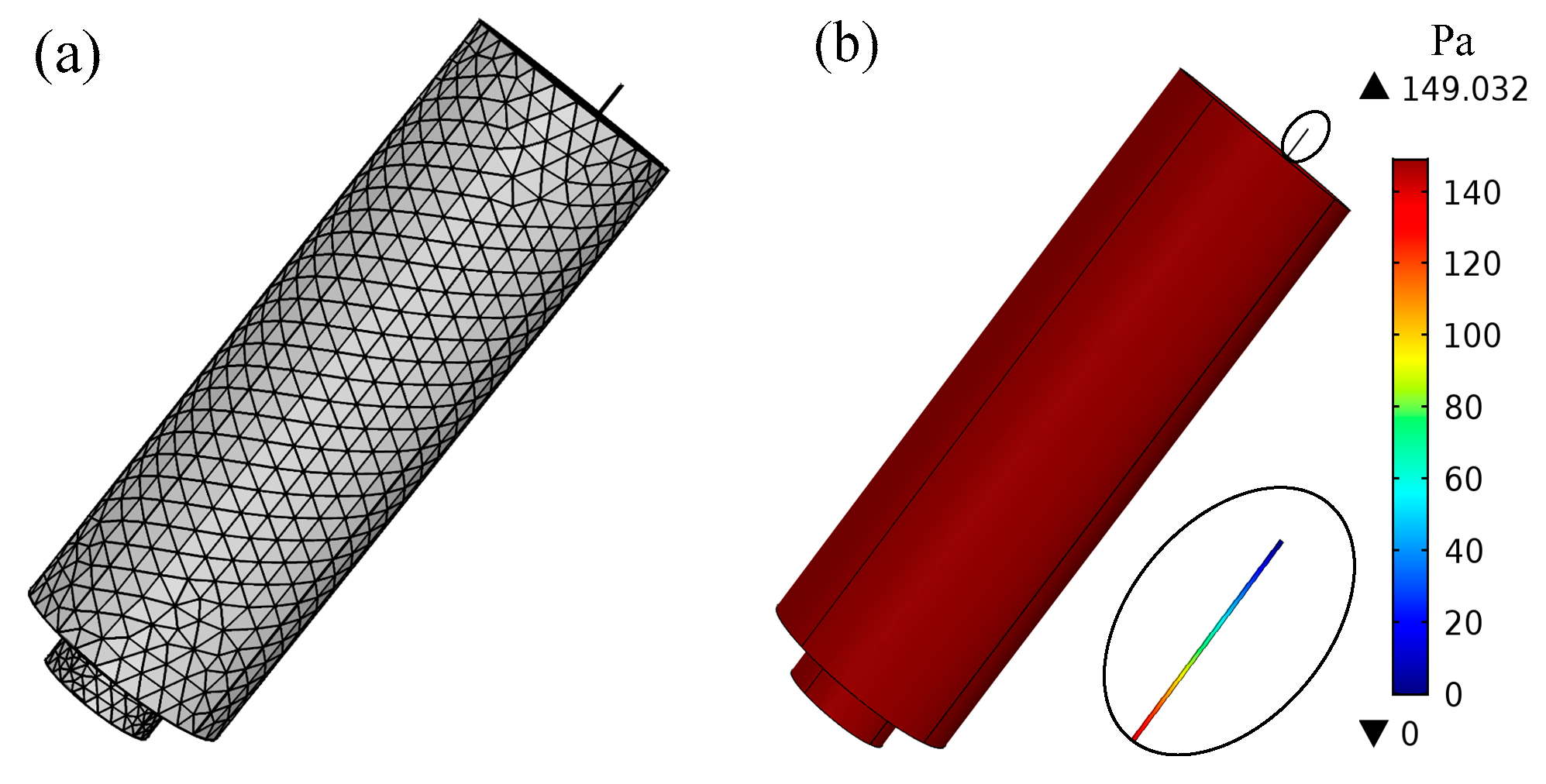
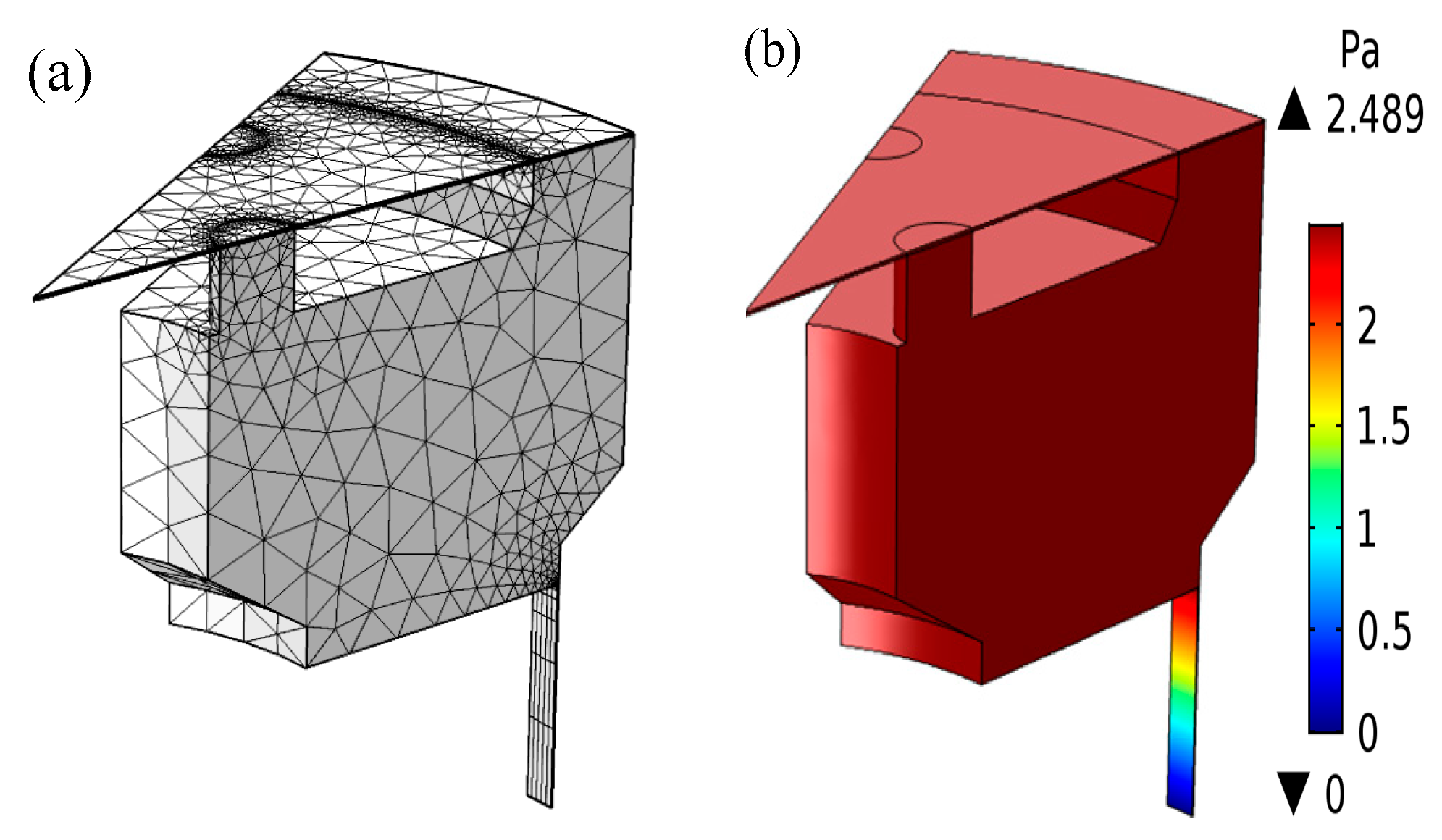
2.1. Model Description

A membrane sealing structure-based pistonphone is designed, as shown in Figure 2 [28]. The cavity is sealed by a silicone membrane, and the piston drives the membrane to vibrate. The cavity wall is made of a seamless steel tube, thus satisfying the rigid wall condition, and produces stable heat conduction. A tiny equalizing hole is opened at the end cover to achieve a static pressure equilibrium. The lower limiting frequency of the pistonphone is about 0.01 Hz and can be further extended by replacing the equalizing hole. All the specific parameters are given in

Table 1. Properties of the laser pistonphone.

Item	Symbol	Value
Chamber radius	R1	65 mm
Chamber length	L1	393 mm
Chamber volume	V0	5.3 × 106 mm3
Diaphragm radius	R2	35 mm
Sealing seat length	L2	24.2 mm
Piston radius	R3	20 mm
Piston internal length	L3	6 mm
Piston displacement	ξpa	5 mm
Equalizing hole radius	R4	0.205 mm
Equalizing hole length	L4	20 mm

.

In the calibration process, except at constant amplitude and zero initial phase with frequency-varying piston displacement excitation, there are pressure leakage, heat conduction, and wave motion effects that affect the phase response between the calibrating sound pressure and the piston displacement. Therefore, four models corresponding to the heat conduction and sealing condition, adiabatic and sealing condition, adiabatic and leaking condition, and heat conduction and leaking condition are respectively established in COMSOL 5.3, as shown in Figure 3. The thermoviscous acoustics modules of both the frequency domain and the transient analysis are used to respectively get the frequency response of the phase difference and the waveform difference between the calibrating sound pressure and the piston displacement [29].

It can be calculated that the temperature change caused by the generated sound pressure is less than 0.2 ℃. Thus, only the effective area of the air in the pistonphone is modeled as shown in Figure 4. Five boundary layers are refined at the surrounding walls to simulate the heat conduction and viscosity loss, and the other remaining area is freely divided into tetrahedral meshes.

For two models considering the pressure leakage effect, the outer end of the equalizing hole is connected to the atmosphere and the boundary condition is set as p_end = 0 Pa. Meanwhile, for two sealing models the outer end is closed. For the other aspect, for two models considering the heat conduction effect, the surrounding walls are set as isothermal—that is, the temperature boundary T_t is always 0. Meanwhile, for two adiabatic models the chamber walls are set as adiabatic—that is, the temperature gradient $-\mathbf{n}·(-k\nabla T_t)=0$, where $\mathbf{n}$ is the normal vector.

At the initial moment, the piston stays at its equilibrium position and outputs a sinusoidal vibration. The amplitude of the piston displacement is selected to be 5 mm, corresponding to a 150 Pa calibrating sound pressure at ideal conditions. In the frequency domain module of COMSOL 5.3, only the amplitude of piston velocity and not the displacement can be applied, and the sine function is set in its background. However, the piston velocity follows the cosine law, and thus will cause severe high-order noise at the time t = 0⁺. To solve this, the velocity amplitude of v = 2πf × 5 [mm] is applied, and the simulated phase results of the calibrating sound pressure at all frequencies are consistently subtracted by 90° to compensate for this model simplification.

The time domain analysis is also conducted by a transient analysis module to reveal the mechanism of phase variation. Only the piston displacement excitation is different from the frequency domain module, as given by $\mathbf{v}=2\mathsf{\pi }f\times 5[\mathrm{mm}]\cos (2\mathsf{\pi }ft)$.

2.2. Results

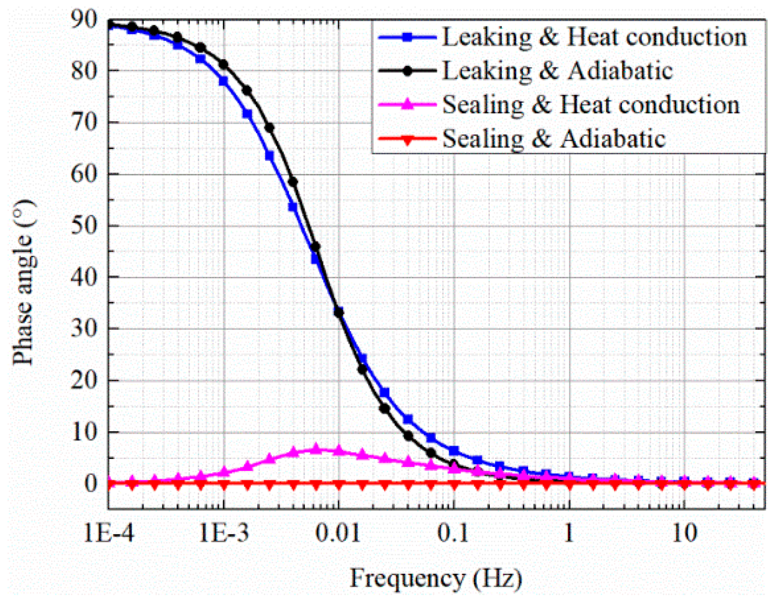
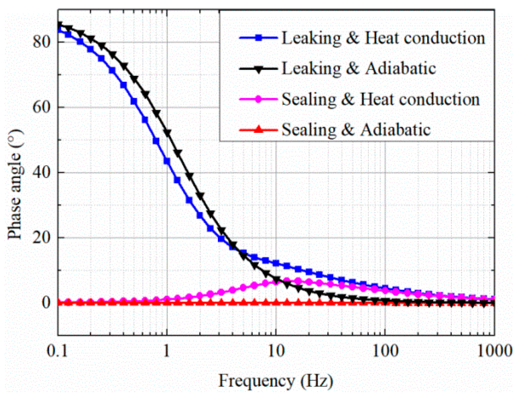
2.2.1. Results in Frequency Domain

The frequency is set from 0.1 mHz to 50 Hz and 1/3 octave for numerical simulation. A probe is inserted at the position where the microphone is installed to get the calibrating sound pressure. The phase difference between the calibrating sound pressure and the piston displacement is the desired phase response of the pistonphone, as given in Figure 5, whose angle is calculated from dividing their time difference by the calibration period and multiplying by 360°. Note that the constant 90° phase compensation has already been done.

As shown in Figure 5, in the ideal sealing and adiabatic conditions the generated sound pressure is exactly synchronized with the piston displacement. The heat conduction effect will cause the phase of the sound pressure to be ahead of the piston displacement, and it works only at middle frequencies. Meanwhile, the effect of the pressure leakage acting on the sound pressure is more obvious and will cause the sound pressure to be 90° ahead of the piston displacement.

The results are clear, but the phase lead phenomenon is quite incomprehensible. Therefore, the following transient simulation is conducted to explain this.

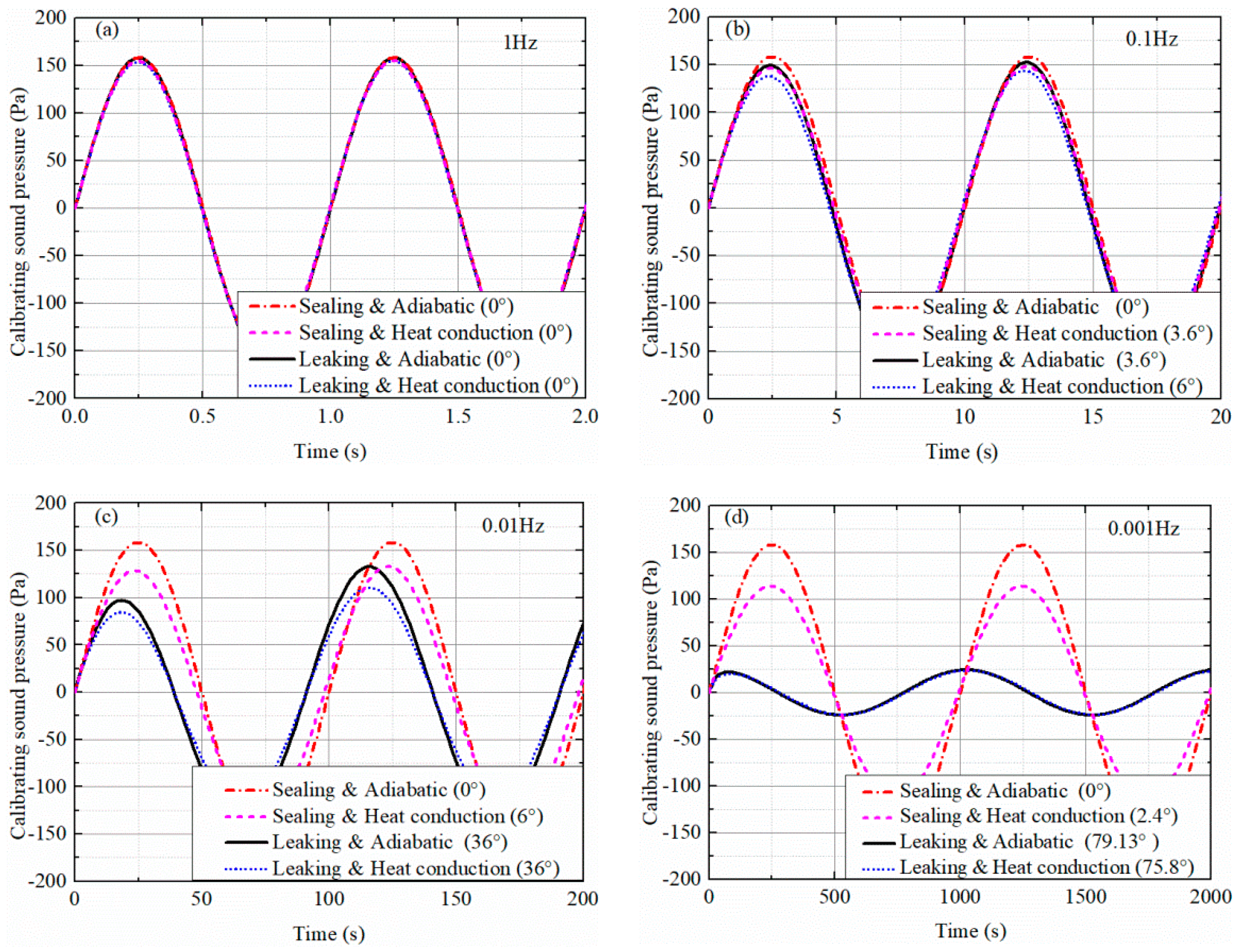
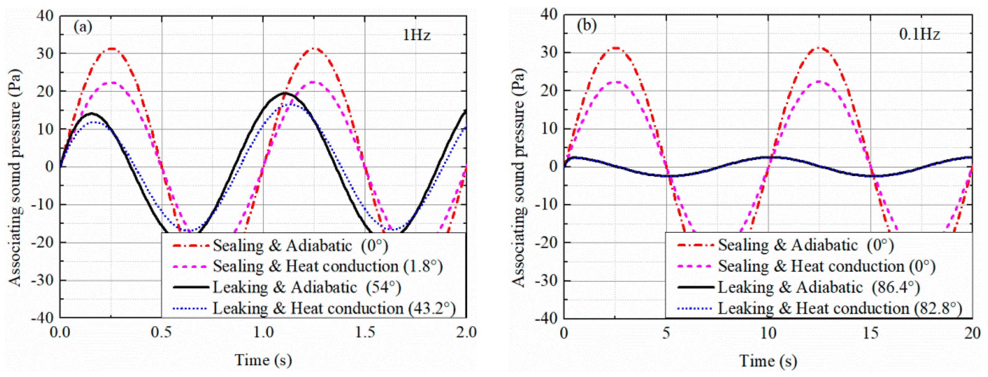
2.2.2. Results in Time Domain

The transient analysis is performed at frequencies of 1 Hz, 0.1 Hz, 0.01 Hz, and 0.001 Hz. The sound pressure waveforms in two cycles are obtained as shown in Figure 6.

Apparently, the sound pressure in the ideal sealing and adiabatic conditions is synchronized with the piston displacement, and thus its waveform can also characterize the waveform of the piston displacement. Then, the phase difference between the sound pressure and the piston displacement in other conditions can be obtained by calculating the time difference of its second peak with that of the sealing and adiabatic condition. The first peak of the waveform is only a transition state and is not selected.

It can be seen that the pressure leakage and heat conduction effects will cause the pressure attenuation, and the phase of the sound pressure will be ahead of the piston displacement rather than lagging behind. The greater the pressure decrease, the greater the phase leading. The angles of the phase lead are calculated and marked in the legends, and the results from the transient analysis are coincident with the frequency domain analysis.

Let us analyze the first three quarters of the first period of the leaking and heat conduction model at 0.001 Hz, as shown in Figure 6d. When the piston sinusoidally moves to its positive extreme position, the increase in the generated sound pressure slows down, and the severe pressure leakage effect causes it to decrease to 0. When the piston moves from this positive extreme position to the negative position, the air would all along be expanded from zero to negative pressure and would have no relation to the equilibrium position of the piston. Therefore, the phase lead of the calibrating sound pressure to the piston displacement occurs.

3. Independent Microphone Simulation

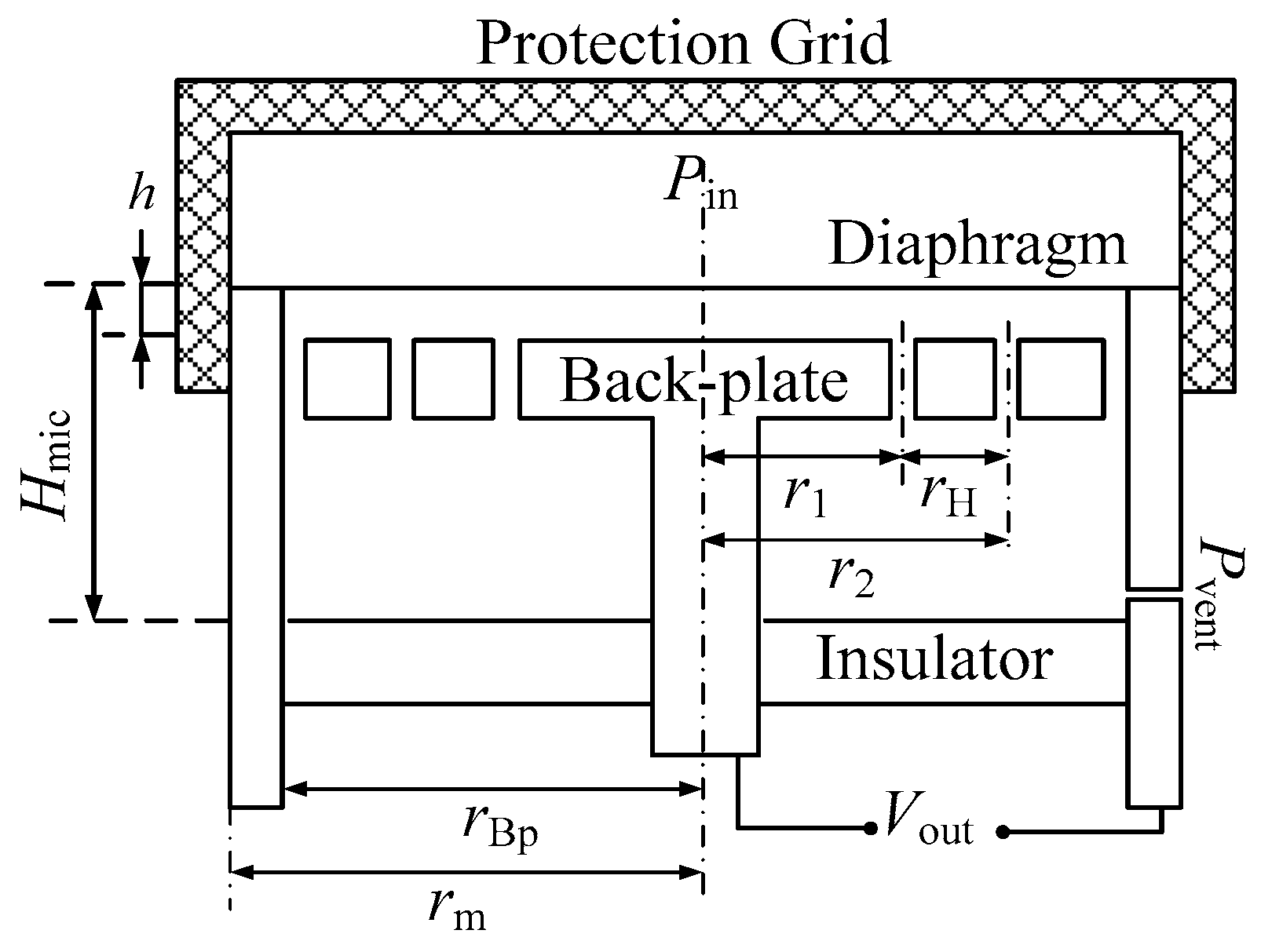
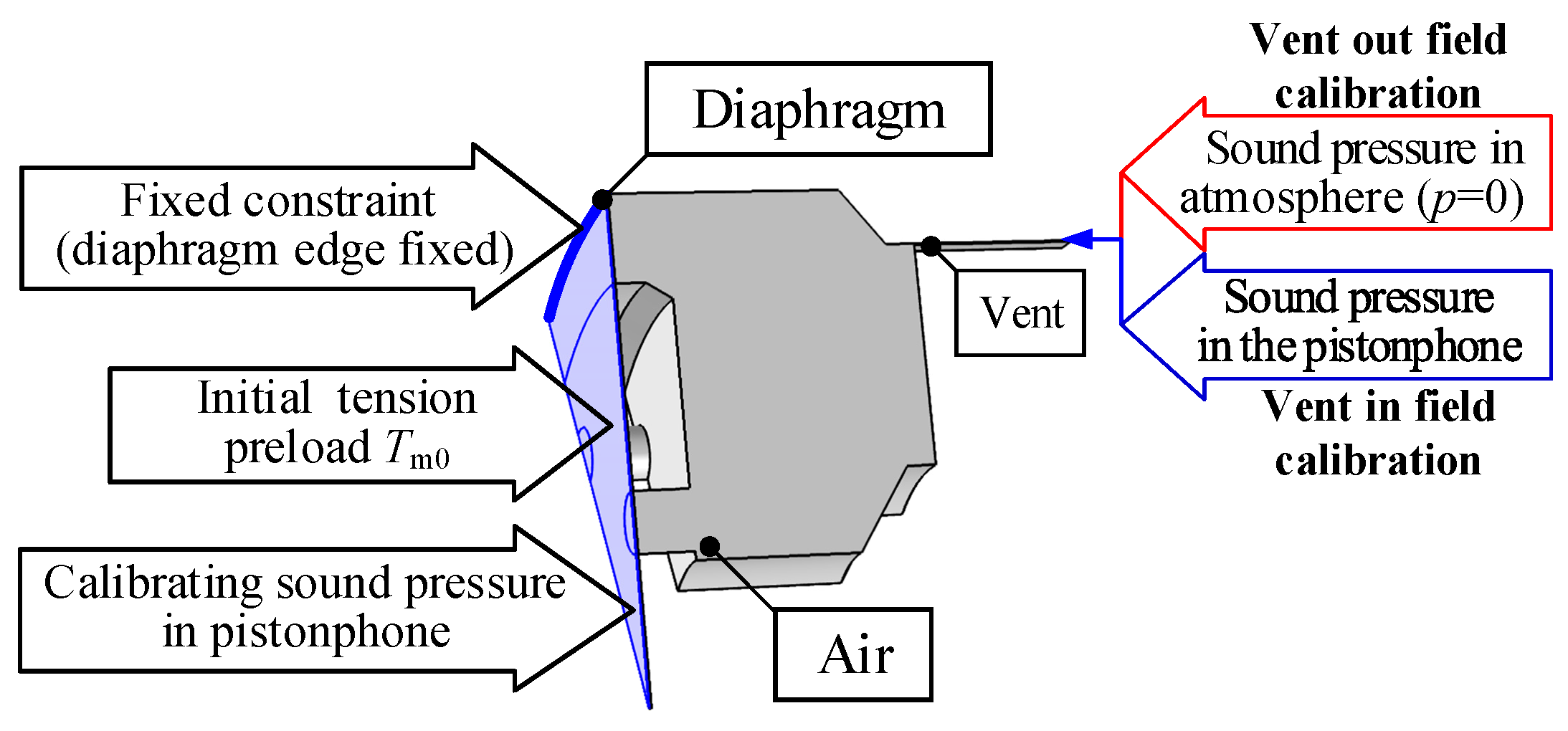
3.1. Model Description

The microphone, as shown in Figure 7, is composed of a diaphragm and a back chamber. A vent is always machined to achieve a static pressure equilibrium in and out of the microphone. When a low-frequency sound excites the diaphragm deformation, the associated sound pressure in the back chamber will also experience pressure leakage and heat conduction effects, so that the phase response of the diaphragm deformation, which is in a linear relationship with the voltage output of the microphone, will be affected [30].

The 1/12 model of the microphone is built as shown in Figure 8. The vent is divided into six sections, and the total acoustic impedance of the six sections is equivalent to the vent [31,32]. Only the effective volume of the air in the back chamber is modeled, and the parameters are consistent with those given in

Table 2. Properties of a microphone.

Item	Symbol	Value
Diaphragm radius	rm	4.5 mm
Diaphragm tension	Tm0	3160 N/m
Diaphragm thickness	tm	5 μm
Diaphragm density	ρm	8900 kg/m3
Gap	h	19 μm
Young’s modulus of diaphragm	Em	2.21 × 1011 Pa
Poisson’s ratio of diaphragm	νm	0.4
Back-plate radius	rBp	3.7 mm
Holes radius	rH	0.28 mm
Location of inner holes	r1	1.6 mm
Location of outer holes	r2	2.8 mm

* Properties of the diaphragm are used in Section 4.

. Proper mesh in the diaphragm region is helpful in correct and fast simulation. Other regions are coarsely meshed, as shown in the figure below.

The boundary conditions of the vent and surrounding walls both for the frequency domain and the transient simulations are the same as the settings of the pistonphone. The velocity excitation is also similar to the settings of the pistonphone, except that a 0.5 μm amplitude excitation is applied to the microphone diaphragm to produce a 32 Pa associated sound pressure at the ideal sealing and adiabatic conditions.

3.2. Results

3.2.1. Results in Frequency Domain

The phase difference between the associated sound pressure and the diaphragm deformation is shown in Figure 9. Due to the smaller chamber, the pressure leakage and heat conduction effects of the microphone are more severe than for the pistonphone. In other words, the phase lead will be larger than that of the pistonphone and will happen at higher frequencies. Therefore, the frequency is set from 0.1 Hz to 1000 Hz and 1/3 octave for the simulation. Note that the constant 90° phase compensation has already been done.

Similar to the trend of the pistonphone, in the ideal sealing and adiabatic conditions the sound pressure is synchronized with the diaphragm excitation. In actual cases, the effect of pressure leakage acting on the sound pressure is more obvious than the heat conduction effect, and will cause the sound pressure to be 90° ahead of the diaphragm deformation at low frequencies. Meanwhile, the heat conduction effect acts only at middle frequencies.

3.2.2. Results in Time Domain

Transient simulations are performed at 0.1 Hz and 1 Hz. The sound pressure waveforms in two cycles are obtained as shown in Figure 10.

Apparently, the pressure leakage and heat conduction effects will not only decrease the amplitude of the generated sound pressure but also result in the phase lead of the diaphragm deformation. A greater pressure attenuation will induce a greater phase lead. The results of the transient and frequency domain analyses can be verified by each other.

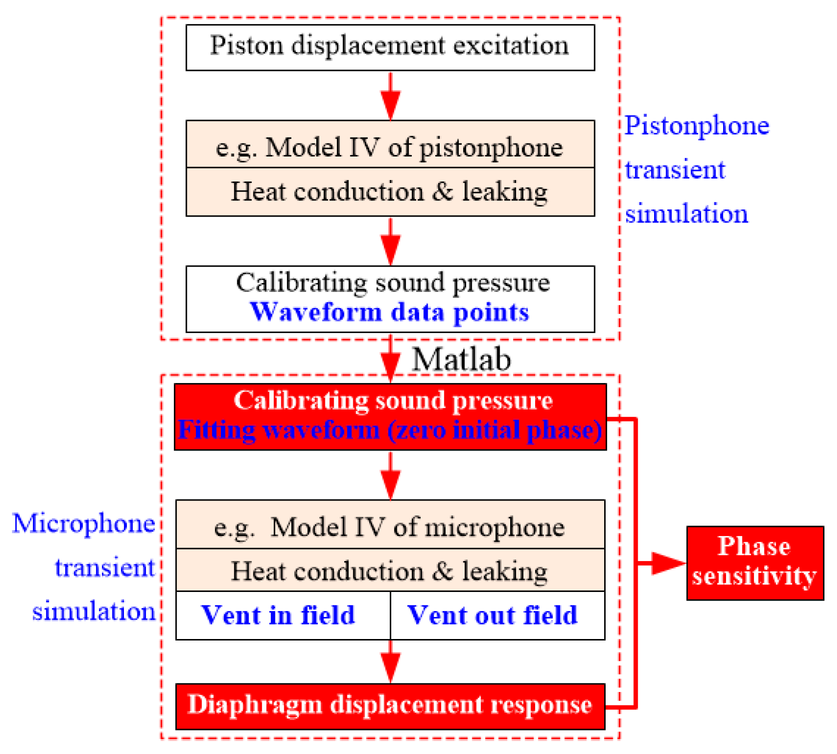
4. Joint Simulation of the Calibration Process

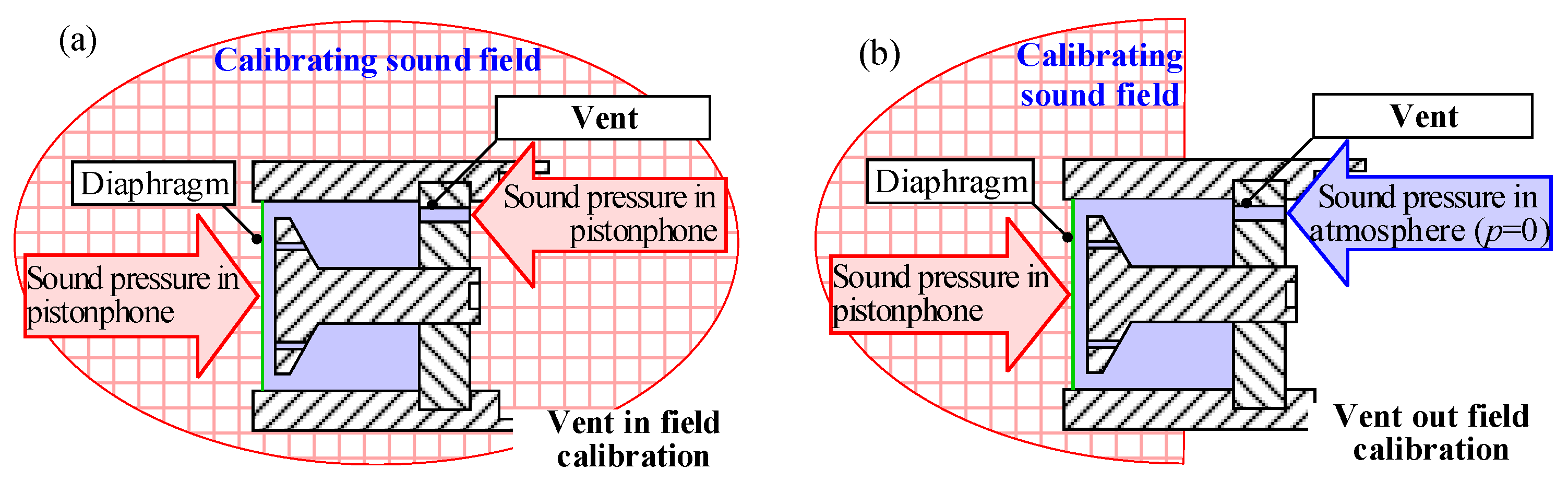
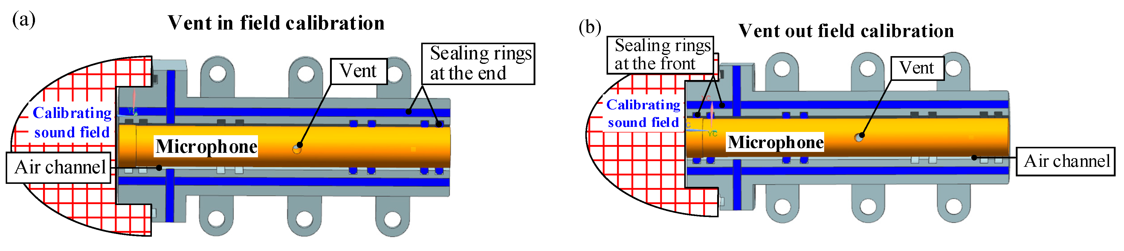
4.1. Model Description

Independent transient simulations for the pistonphone and microphone, as shown in Figure 6 and Figure 10, show that the sound pressure amplitude of both the pistonphone and the microphone will decrease at low frequencies. Meanwhile, the phase will be ahead of their excitation. Due to the more severe pressure leakage and heat conduction loss in the microphone, the amplitude attenuation and phase lead are earlier in microphone than in pistonphone, and thus the phase variation in microphone sensitivity will happen at low frequencies.

The key to the simulation of the primary calibration process is to apply the calibrating sound pressure in the pistonphone to the microphone diaphragm. However, the size difference between the pistonphone and the microphone is quite large; in particular, the equalizing hole of pistonphone, the vent of microphone, and the gap between the diaphragm and the back-plate are only several microns. If two models are directly coupled, the calculation is computationally expensive. Therefore, a joint simulation method is adopted to firstly calculate the calibrating sound pressure in the pistonphone and then add it to the diaphragm of the microphone model to obtain the desired phase sensitivity of the microphone.

In addition, depending on whether the vent of microphone is installed in or out of the calibrating field during calibrations, as shown in Figure 11, the calibration results will be very different. Thus, these two calibration states are studied. For vent in field calibrations, the sound pressure in the pistonphone is quite uniform at low frequencies, so that the incident sound pressure on the diaphragm and the outer end of the vent are both the calibrating sound pressure obtained from the independent pistonphone simulation. Meanwhile, for vent out field calibrations the incident sound pressure on the outer end of the vent is 0.

The “Structural mechanics, diaphragm” interface is now added to the microphone model to apply the calibrating sound pressure on the diaphragm, as shown in Figure 12. The edge of the diaphragm is set fixed and a tension preload T_m0 is applied to it. The “thermosviscous acoustics-structure boundary” coupling module is used to couple the diaphragm and the sound field. The “Moving Mesh” interface is used to accurately simulate the diaphragm vibration [33].

When the electrical characteristics of the microphone and its matched preamplifier are considered as constant, the diaphragm deformation of the microphone is equivalent to its voltage output. Therefore, the phase difference between the diaphragm deformation of the microphone and the calibrating sound pressure in the pistonphone is the desired phase sensitivity of the microphone.

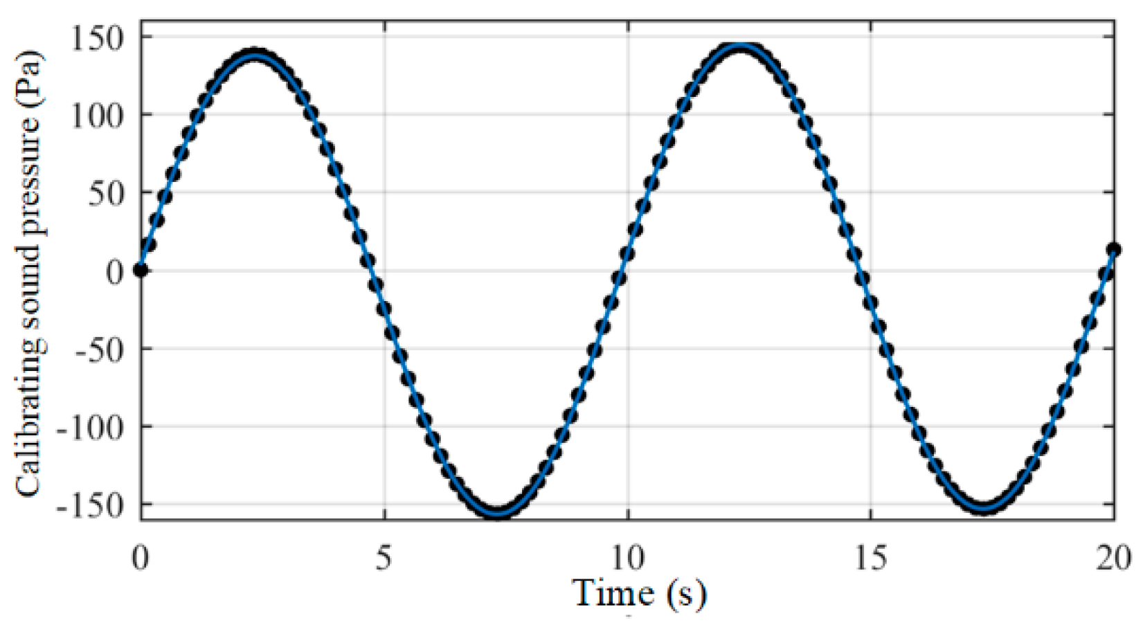
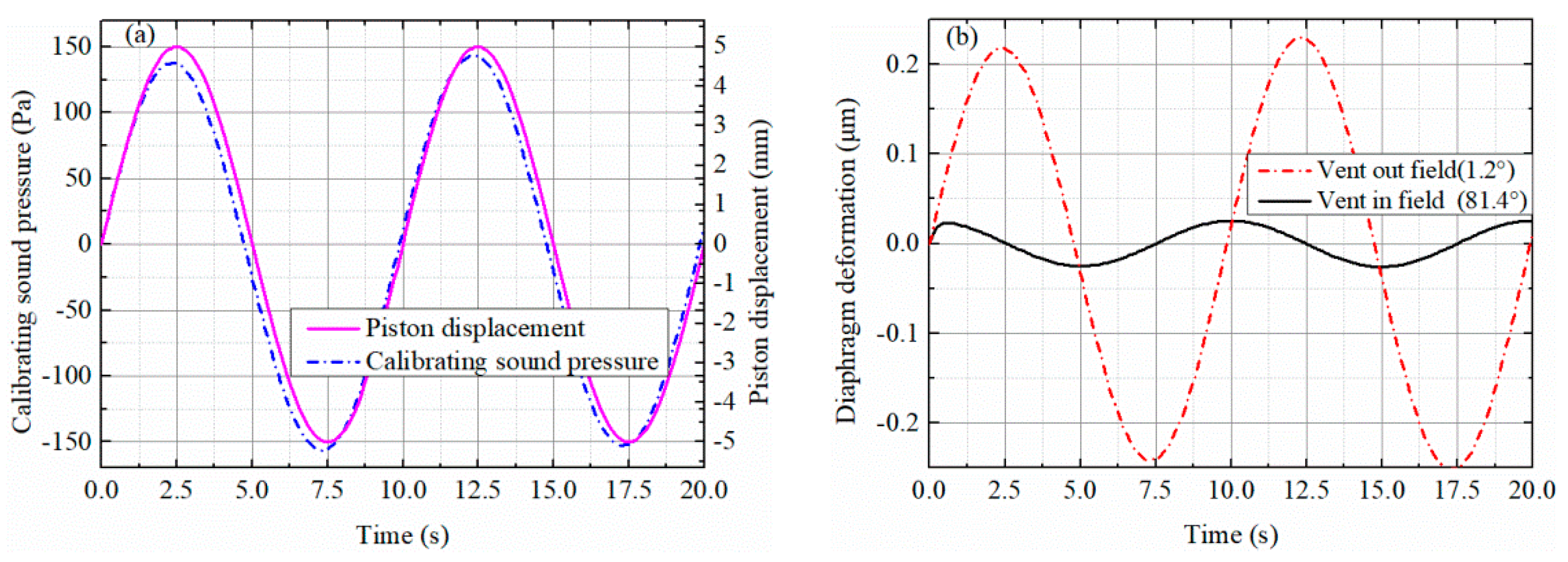
4.2. Time Domain Simulation

The joint simulation in the time domain needs to apply the time-varying calibrating sound pressure, as shown in Figure 6, to the microphone diaphragm. The sound pressure has not only an amplitude attenuation but also a phase lead against the piston excitation. Since the phase sensitivity is the time difference between the calibrating sound pressure and the microphone voltage, the initial phase of the sound pressure needs to be wiped off. Therefore, the corrected waveform of the sound pressure is fitted to the spline curve and then added to the microphone diaphragm to conduct the simulation. The flow chart of the time domain joint simulation is shown in Figure 13.

Taking the calibration process at 0.1 Hz as an example, the second order Fourier series is used to fit the waveform of the calibrating sound pressure, as shown in Figure 14.

The fitting formula is given by:

$$p=a_0+a_1\cos (\omega t)+b_1\sin (\omega t)+a_2\cos (2\omega t)+b_2\sin (2\omega t),$$

(5)

where a₀ = −7.069, a₁ = −1.353, a₂ = 11.58, b₁ = −3.654, b₂ = 147.3, and ω = 0.3156 rad/s.

An independent pistonphone simulation at 0.1 Hz is first conducted to obtain the waveform of the piston displacement and the calibrating sound pressure, as shown in Figure 15a. Secondly, the fitting waveform of the calibrating sound pressure is added to the microphone diaphragm and microphone simulations in both the vent in field and vent out field states are conducted. The diaphragm deformation of the microphone in the two venting states is shown in Figure 15b.

By calculating the time difference of the second peak of the voltage output with that of the calibrating sound pressure, the phase sensitivities of the microphone for the vent in field and vent out field calibrations are calculated as 1.2° and 81.4°, respectively. It is clear that the microphone phase sensitivities in the two venting states are quite different at low frequencies.

It can be seen that the diaphragm deformation of the vent in the field calibration shows a more severe attenuation and phase lead than the vent out field calibration at low frequencies. That is because, for the vent in field calibration, the vent end is in the pistonphone chamber and bears the calibrating sound pressure with only a certain delay due to the vent resistance, so that the microphone output decreases a lot and the 81.4° phase lead occurs.

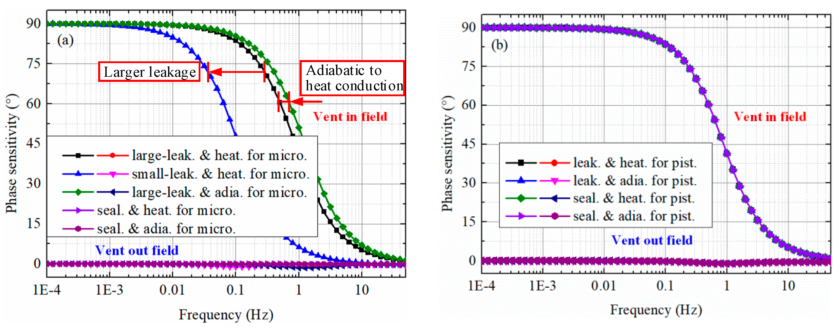
4.3. Frequency Domain Simulation

The time domain simulation can only get the phase sensitivity at a certain frequency, while the frequency domain simulation will give the whole picture of it, so this is further conducted.

Firstly, the influence of the microphone geometries on the phase sensitivity of the microphone is studied, as shown in Figure 16a, while the pistonphone model adopts more realistic heat conduction and leaking conditions. The sealing features of the microphone are labeled as sealing (seal.), small leaking (small-leak.) and large leaking (large-leak.). Meanwhile, the heat conduction features are labeled as adiabatic (adia.) and heat conduction (heat.).

Secondly, the influence of the pistonphone geometries on the phase sensitivity of the microphone is studied, as shown in Figure 16b, while the microphone model adopts more realistic heat conduction and leaking conditions. The sealing features of the pistonphone are labeled as sealing (seal.) and leaking (leak.).

From Figure 16, it can be found that the microphone phase sensitivity for the vent in field and vent out field calibrations differ greatly at low frequencies. A phase lead limit of 90° will happen for the vent in field calibration at very low frequencies, while it is almost unaffected for the vent out field calibrations. The tiny phase lag for the vent out field calibrations is caused by the diaphragm pushing the air flow through the hole into the atmosphere. Thus, a sealed microphone will not have such a phenomenon.

Figure 16a shows the influence of the pressure leakage and heat conduction effects in the microphone back chamber on its phase sensitivity, while Figure 16b shows the influence of the pressure leakage and heat conduction effects in the pistonphone on the microphone phase sensitivity. It can be concluded that the pressure leakage loss in the microphone back chamber is the dominating factor that affects its phase sensitivity in the vent in field calibrations, while the influence of the heat conduction effect on the phase sensitivity is much less. The properties of the pistonphone will not affect the phase sensitivity of the microphone.

4.4. Verification and Planning

The above studies in this paper are pure FEA simulations. It is more convincing if the same phenomenon can be found experimentally. To the best of our knowledge, the only study that can partially prove our study is by Franck Larsonner et al., who calibrated the phase frequency response of MB2005 and MB3 microbarometers. The amplitude and phase responses of the MB2005 microbarometer and the MB3 microbarometer shows the same tendency [15]. Apparently, the low-frequency phase characteristics of both microbarometers show a typical phase leading phenomenon. This is in good agreement with the results of the vent in field calibration, as shown in Figure 16. However, the results of the vent out field calibration are not given, which may be because the microbarometers are only used in the air and will be wholly placed in the sound field. Thus, the vent out field calibrations are not conducted.

To verify the phase sensitivity of the microphone at low frequencies, an experimental plan is briefly given as follows. A low frequency microphone with matched preamplifiers (PCD 378A07 and 426E01) will be selected as the research object. A special mounting seat, which can realize both the vent in field and vent out field calibrations, should be manufactured as shown in Figure 17. The vibration displacement waveform of the piston will be measured by the laser vibrometer, as shown in Figure 1. A phase comparison between the voltage output of the microphone and the vibration displacement of the piston will be made to verify the correctness of the simulation. The above experimental study will be the next major work for our team.

5. Conclusions

The low frequency phase characteristics of microphones are crucial for large-scale natural and artificial activity measurements, but their primary calibrations have been grossly overlooked. By means of the FEA technique, this paper studies the laser pistonphone-based primary calibration of microphones and finds that the generated sound pressures in both the pistonphone and microphone show an interesting phase lead (relative to the displacement excitation) at low frequencies due to the dominating pressure leakage loss. The diaphragm deformation of the microphone is then affected, and its sensitivity varies at low frequencies. Depending on whether its vent is inserted in the calibrating sound field or in the outside atmosphere, there are two very different phase sensitivity responses of the microphone. A phase lead limit of 90° will happen in vent in field calibrations, but the phase lead is almost unaffected in vent out field calibrations. Therefore, depending on whether the low-frequency sound in air or in duct is to be measured, the corresponding sensitivities of the microphone should be selected as the correction standard.

Different from the in situ calibration and calibrator methods, which give only the phase consistencies of the microphones, the primary calibration-determined phase sensitivity of the microphone shows its intrinsic characteristics, and will not be affected by the installation change of the monitoring system. Therefore, it is recommended to obtain the primary phase sensitivity of the microphone before serving.

References

1. Seo, S.-W.; Yun, S.; Kim, M.-G.; Sung, M.; Kim, Y. Screen-Based Sports Simulation Using Acoustic Source Localization. Appl. Sci. 2019, 9, 2970. [Google Scholar] [CrossRef] [Green Version]
2. Cheng, R.; Bao, C.; Cui, Z. MASS: Microphone Array Speech Simulator in Room Acoustic Environment for Multi-Channel Speech Coding and Enhancement. Appl. Sci. 2020, 10, 1484. [Google Scholar] [CrossRef] [Green Version]
3. Ferguson, B.; Gendron, P.; Michalopoulou, Z.H.; Wong, K.T. Introduction to the special issue on acoustic source localization. J. Acoust. Soc. Am. 2019, 146, 4647–4649. [Google Scholar] [CrossRef] [PubMed]
4. Krishnappa, G. Cross-spectral method of measuring acoustic intensity by correcting phase and gain mismatch errors by microphone calibration. J. Acoust. Soc. Am. 1981, 69, 307–310. [Google Scholar] [CrossRef]
5. Chen, X.; Chen, Y.H.; Cao, S.; Zhang, L.; Zhang, X.; Chen, X. Acoustic indoor localization system integrating TDMA+FDMA transmission scheme and positioning correction technique. Sensors 2019, 19, 2353. [Google Scholar] [CrossRef] [Green Version]
6. Groot-Hedlin, C.D.D.; Hedlin, M.A.H.; Drob, D.P. Infrasound Monitoring for Atmospheric Studies; Springer: Dordrecht, The Netherlands, 2010. [Google Scholar]
7. Sciotto, M.; Cannata, A.; Gresta, S.; Privitera, E.; Spina, L. Seismic and infrasound signals at Mt. Etna: Modeling the north-east crater conduit and its relation with the 2008–2009 eruption feeding system. J. Volcanol. Geoth. Res. 2013, 254, 53–68. [Google Scholar] [CrossRef] [Green Version]
8. Gitterman, Y.; Hofstetter, R. GT0 explosion sources for IMS infrasound calibration: Charge design and yield estimation from near-source observations. Pure Appl. Geophys. 2014, 171, 599–619. [Google Scholar] [CrossRef]
9. Adin Mann, J., III; Pascal, J.C.; Phan, T.M. Low frequency correction of electrostatic microphone pair phase calibration. In Proceedings of the INTER-NOISE and NOISE-CON Congress and Conference Proceedings, InterNoise90, Gothenburg, Sweden, 13 August 1990; pp. 1057–1060. [Google Scholar]
10. Lowis, C.R.; Joseph, P.F.; Sijtsma, P. A technique for the in situ phase calibration of in-duct axial microphone arrays. J. Sound Vib. 2010, 329, 4634–4642. [Google Scholar] [CrossRef]
11. Lauterbach, A.; Ehrenfried, K.; Koop, L.; Loose, S. Procedure for the accurate phase calibration of a microphone array. In Proceedings of the Aiaa/ceas Aeroacoustics Conference & Aiaa Aeroacoustics Conference, Miami, FL, USA, 11–13 May 2009. [Google Scholar]
12. Rasmussen, G.; Nielson, K.M. Technical note low frequency calibration of measurement microphones. J. Low Freq. Noise Vib. Act. Control 2009, 28, 223–228. [Google Scholar] [CrossRef]
13. Kutin, J.; Bajsić, I. Characteristics of a dynamic pressure generator based on loudspeakers. Sens. Actuators A-Phys. 2011, 168, 149–154. [Google Scholar] [CrossRef]
14. Štefe, M.; Svete, A.; Kutin, J. Development of a dynamic pressure generator based on a loudspeaker with improved frequency characteristics. Measurement 2018, 122, 212–219. [Google Scholar] [CrossRef]
15. Larsonner, F.; Uszakiewicz, H.G.; Mende, M. Infrasound sensors and their calibration at low frequency. In Proceedings of the INTER-NOISE and NOISE-CON Congress and Conference Proceedings, InterNoise14, Melbourne, Australia, 1 January 2014; pp. 1127–1136. [Google Scholar]
16. Infrasound sensor. Available online: http://blog.sina.com.cn/s/blog_67cd56c10100iuaj.html (accessed on 14 May 2010).
17. Tóth, P.; Schram, C. Simultaneous calibration of multiple microphones for both phase and amplitude in an impedance tube. Arch. Acoust. 2014, 39, 227–287. [Google Scholar] [CrossRef] [Green Version]
18. Scott, D.A.; Dickinson, L.P.; Ballico, M.J. Traceable calibration of microphones at low frequencies. Meas. Sci. Technol. 2019, 30, 035011. [Google Scholar] [CrossRef]
19. International Electrical Commission. 2009 Electroacoustics—Measurement Microphones—Primary Method for Pressure Calibration of Laboratory Standard Microphones by the Reciprocity Technique IEC 61094-2:2009. 2009. Available online: https://webstore.iec.ch/publication/4486 (accessed on 15 May 2020).
20. Nel, R.; Van Zyl, B.G.; Snyman, L.W. Analysing the effects of phase sensitivity in low frequency primary microphone calibrations. Appl. Acoust. 2017, 127, 95–104. [Google Scholar] [CrossRef]
21. Jackett, R.J.; Barham, R.G. Phase sensitivity uncertainty in microphone pressure reciprocity calibration. Metrologia 2013, 50, 170–179. [Google Scholar] [CrossRef]
22. Barham, R.G.; Goldsmith, M.J. The application of the NPL laser pistonphone to the international comparison of measurement microphones. Metrologia 2007, 44, 210–216. [Google Scholar] [CrossRef]
23. Sadıkoğlu, E.; Bilgiç, E.; Karaböce, B. A laser pistonphone based on self-mixing interferometry for the absolute calibration of measurement microphones. Appl. Acoust. 2004, 65, 833–840. [Google Scholar] [CrossRef]
24. Rennie, A.J. A laser-pistonphone for absolute calibration of laboratory standard microphones in the frequency range 0.1 Hz to 100 Hz. NPL Acoust. Rep. Ac. 1977, 78, 23410. [Google Scholar]
25. He, W.; He, L.B.; Zhang, F.; Rong, Z.; Jia, S. A dedicated pistonphone for absolute calibration of infrasound sensors at very low frequencies. Meas. Sci. Technol. 2016, 27, 025018. [Google Scholar] [CrossRef]
26. Wong, G.S.K.; Embleton, T.F.W. AIP handbook of condenser microphones: Theory, calibration, and measurements. J. Acoust. Soc. Am. 1995, 98, 171–172. [Google Scholar]
27. Zhang, F.; He, W.; He, L.B.; Rong, Z. Acoustic properties of pistonphones at low frequencies in the presence of pressure leakage and heat conduction. J. Sound Vib. 2015, 358, 324–333. [Google Scholar] [CrossRef]
28. Liu, D.; Liu, A.B.; Zhang, F.; Gang, X.; Li, L.; Wu, H. A dynamic pressure calibration device based on the low speed servomotor and pistonphone technique. Measurement 2020, 151, 107254. [Google Scholar] [CrossRef]
29. The “Thermoviscous Acoustics Branch” section in the Acoustics Module User’s Guide of the COMSOL Documentation. Available online: https://doc.comsol.com/5.4/doc/com.comsol.help.aco/AcousticsModuleUsersGuide.pdf (accessed on 15 May 2020).
30. Brüel and Kjær. Microphone Handbook—Vol. 1: Theory. Technical Documentation. 1996. Available online: https://www.bksv.com/media/doc/be1447.pdf (accessed on 15 May 2020).
31. Homentcovschi, D.; Miles, R.N. An analytical-numerical method for determining the mechanical response of a condenser microphone. J. Acoust. Soc. Am. 2011, 130, 3698–3705. [Google Scholar] [CrossRef] [PubMed] [Green Version]
32. Lavergne, T.; Durand, S.; Bruneau, M.; Joly, N. Dynamic behavior of the circular membrane of an electrostatic microphone: Effect of holes in the backing electrode. J. Acoust. Soc. Am. 2010, 128, 3459–3477. [Google Scholar] [CrossRef] [PubMed]
33. The Brüel & Kjær 4134 Condenser Microphone. Available online: https://www.comsol.it/model/the-br-252-el-kj-230-r-4134-condenser-microphone-12375 (accessed on 29 May 2020).
Figure 1. (a) The calibration characteristics of the laser pistonphone technique. (b) Prototype of a laser pistonphone.
Applsci 10 03799 g001
Figure 2. Schematic diagram of the pistonphone chamber.
Applsci 10 03799 g002
Figure 3. Flow chart of the pistonphone simulation.
Applsci 10 03799 g003
Figure 4. (a) The FEA model of the pistonphone. (b) Sound pressure distribution for the heat conduction and leaking condition at 0.1 Hz.
Applsci 10 03799 g004
Figure 5. Phase difference between the calibrating sound pressure and the piston displacement.
Applsci 10 03799 g005
Figure 6. (a) Sound pressure waveforms of the calibrating sound pressure at 1 Hz. (b) Sound pressure waveforms of the calibrating sound pressure at 0.1 Hz. (c) Sound pressure waveforms of the calibrating sound pressure at 0.01 Hz. (d) Sound pressure waveforms of the calibrating sound pressure at 0.001 Hz.
Applsci 10 03799 g006
Figure 7. Assembly drawing of a condenser microphone.
Applsci 10 03799 g007
Figure 8. (a) The FEA model of the microphone. (b) Sound pressure distribution for the heat conduction and leaking condition at 0.1 Hz, in which the sound pressure decreases to almost 0.
Applsci 10 03799 g008
Figure 9. Phase difference between the associated sound pressure and the diaphragm deformation of the microphone.
Applsci 10 03799 g009
Figure 10. (a) Sound pressure waveforms of the associated sound pressure at 1 Hz. (b) Sound pressure waveforms of the associated sound pressure at 0.1 Hz.
Applsci 10 03799 g010
Figure 11. (a) Calibration in which the outer end of the vent is inserted in the calibrating sound field. (b) Calibration in which the outer end of vent is in the outside atmosphere.
Applsci 10 03799 g011
Figure 12. Multi-physical joint simulation of the microphone primary calibration.
Applsci 10 03799 g012
Figure 13. Flow chart of the time domain simulation.
Applsci 10 03799 g013
Figure 14. Waveform fitting at 0.1 Hz.
Applsci 10 03799 g014
Figure 15. (a) Waveform of the piston displacement and the calibrating sound pressure at 0.1 Hz. (b) Waveform of the diaphragm deformation at 0.1 Hz in two venting states.
Applsci 10 03799 g015
Figure 16. (a) Phase sensitivity of the microphone in two venting states, in which the properties of the microphone change. (b) Phase sensitivity of the microphone in two venting states, in which the properties of the pistonphone change.
Applsci 10 03799 g016
Figure 17. (a) Planned vent in field calibration. (b) Planned vent out field calibration.
Applsci 10 03799 g017