Abstract
This paper presents a statistical model to estimate the volume of released tailings (VF) and the maximum distance travelled by the tailings (Dmax) in the event of a tailings dam failure, based on physical parameters of the dams. The dataset of historical tailings dam failures is updated from the one used by Rico et al., (Floods from tailings dam failures, Journal of Hazardous Materials, 154 (1) (2008) 79–87) for their regression model. It includes events out of the range of the dams contained in the previous dataset. A new linear regression model for the calculation of Dmax, which considers the potential energy associated with the released volume is proposed. A reduction in the uncertainty in the estimation of Dmax when large tailings dam failures are evaluated, is demonstrated. Since site conditions vary significantly it is important to directly consider the uncertainty associated with such predictions, rather than directly using these types of regression equations. Here, we formally quantify the uncertainty distribution for the conditional estimation of VF and Dmax, given tailings dam attributes, and advocate its use to better represent the tailings dam failure data and to characterize the risk associated with a potential failure.
1. Introduction
The failure of tailings storage facilities can have disastrous consequences for nearby communities, the environment, and for the mining companies, who may consequently face high financial and reputational costs. Tailings are waste resulting from mining operations and are commonly deposited as slurry behind earthen or masonry dams. We refer to this form of tailing storage facility as TSF. In 2015, the breach of the Fundão TSF at Samarco mine in Minas Gerais (jointly owned by BHP Billiton Brasil and Vale S.A.) resulted in 19 fatalities, and was declared the worst environmental disaster in Brazil’s history. The company entered an agreement with the Federal Government of Brazil and other public authorities to remediate and compensate for the impacts over a 15 years period. Jointly, BHP and Vale recognized a US$ 2.4 billion provision for potential obligations under the agreement [1,2]. Twenty-one company executives were charged with qualified murder, and up until September 2017 the mine had not resumed operations. The ecosystems impacts caused by a TSF failure can last for many years depending on the nature of the tailings. Samarco is in the process of restoring 5000 streams, 16,000 hectares of Permanent Conservation Areas along the Doce River basin, and 1200 hectares in the riverbanks [3]. It is estimated that the livelihoods of more than 1 million people were affected because of the failure [4]. Improvements in the design, monitoring, management, and risk analysis of TSFs are needed to prevent future failures and to estimate the consequences of a breach.
The design of tailings dams has changed significantly from the 1930s to the present [5,6,7]. Construction of the early TSFs was done by trial and error [8]. During the 1960’s and 1970’s geomechanical engineering started to be used to assess the behavior of the tailings and the stability of the impoundments [8]. Currently, various studies are required to approve a TSF design and increasingly the plans for remediation and closure of the impoundments have to be included in the feasibility phase. Breach assessments are now part of the requirements in the permitting process of a new TSF or an expansion in many countries. Different parameters need to be estimated while conducting these assessments [9]. These include the volume of tailings (VF) that could potentially be released, and the distance to which the material may travel in a downstream channel, called the run-out distance (Dmax). Empirical regression equations for this purpose were developed by Rico et al. [10] using historical TSF failure data, and are commonly used to characterize such failures (similar empirical relationships have been developed for dams holding water [11,12], but the lack of tailings and differences in design and construction make them inapplicable to tailings dams). However, at site conditions in the mines can vary substantially and there is considerable residual uncertainty associated with the conditional mean value estimated by these equations. In this paper, we rigorously update these regression equations using an updated data set, and characterize the uncertainty associated with the prediction. Using the uncertainty distribution for the conditional estimation of VF and Dmax using TSF parameters provides a better way to interpret the TSF failure data and to characterize the risk associated with a potential failure.
The calculation of VF is of particular importance for inundation analyses. Typically, TSFs are not totally emptied in case of failure (as opposed to water dams), and only a portion of the tailings are released [10]. In TSFs containing a large amount of water (supernatant pond), the breach would usually result in an initial flood wave followed by mobilized/liquefied tailings [9]. Therefore, the methods developed to estimate the released volume of water or the inundation extent from a regular dam (such as the water dam break-flood analyses methods in [13,14]), do not apply to tailings dams. Empirical equations based on past failures, dam height, and the impounded volume of tailings, are commonly used to get a first estimate of the volume of tailings that could be released and the run-out distance. In Rico et al. [10] VF is calculated using the total impounded volume (VT) in Mm3 as in Equation (1)
and the outflow run-out distance travelled by the tailings in km (Dmax) is obtained using VF and the dam’s height in meters at the time of failure (H) as in Equation (2)
Many investigators directly use such regression equations in a deterministic way to specify exposure. However, at site conditions vary significantly, and there is considerable uncertainty that needs to be quantified. This uncertainty increases as we consider TSF volumes that are near or beyond the range of the data included in the regression equation. Equation (1) predicts that approximately a third of the tailings in the impoundment (including water) will be the outflow volume. This approach may result in unrealistic estimates when liquefaction is a known risk as it does not take into account the tailings mass rheology (viscosity and yield stress) [9]. As Rico et al. [10] point out, some parameters contributing to the uncertainty in the predictions include sediment load, fluid behavior (depending on the type of failure), topography, the presence of obstacles stopping the flow, and the proportion of water stored in the tailings dam (linked to meteorological events or not). Therefore, it is important to account for the uncertainty in these estimates to derive a probabilistic measure of risk that also accounts for how well the regression fits in a certain range of values of the predictors.
Additional information about TSF failures since Rico et al. [10] published the above-mentioned equations is available. In this paper we update the original data used by Rico from 22 complete cases (including height, storage volume in m3, released volume in m3, and distance traveled) to 29 complete cases with data compiled in Chambers and Bowker [15]. We compare the results of the original linear regressions done by Rico et al. [10] with the results using the updated dataset. A new model for the calculation of Dmax is proposed introducing the predictor (Hf), which is defined as:
This variable was introduced to consider that the potential energy associated with the release volume, may be better related to the fractional volume released as opposed to the total volume of the TSF.
For each of the models we consider, and for the final model we recommend, we consider the uncertainty analysis of prediction. We compare the predicted intervals and observed values of VF and Dmax of three TSF failures across the models that were evaluated to see how well the prediction intervals fit the observed data. The indicated probability of exceedance of the observation as per each model was also assessed.
2. Materials and Methods
The height at time of failure (H), TSF capacity (VT), released volume (VF), and the distance traveled by the tailings (Dmax) are inputs in Rico’s equations (Equation (1) and Equation (2)). The data used in this analysis is a combination of the cases used by Rico and others compiled by Chambers and Bowker [15], including failures post 2008. Seven of the 29 incidents used by Rico et al. [10] do not have complete information or the information for volume is included in million tons, which cannot be used in the analysis without density data. These cases are in red letters in Table 1. It is important to note that the original data did not include releases as large as the ones experienced in Samarco and Mt Polley (cases 15 and 19 in Table 1), and this becomes relevant for future estimations of the potential risk of larger TSFs. The data on reported failures have variations in different sources; some of these variations are included as footnotes in Table 1.

Table 1.
Data in Rico et al. [10] and Chambers and Bowker (CB) [15]. Entries in red are incomplete.
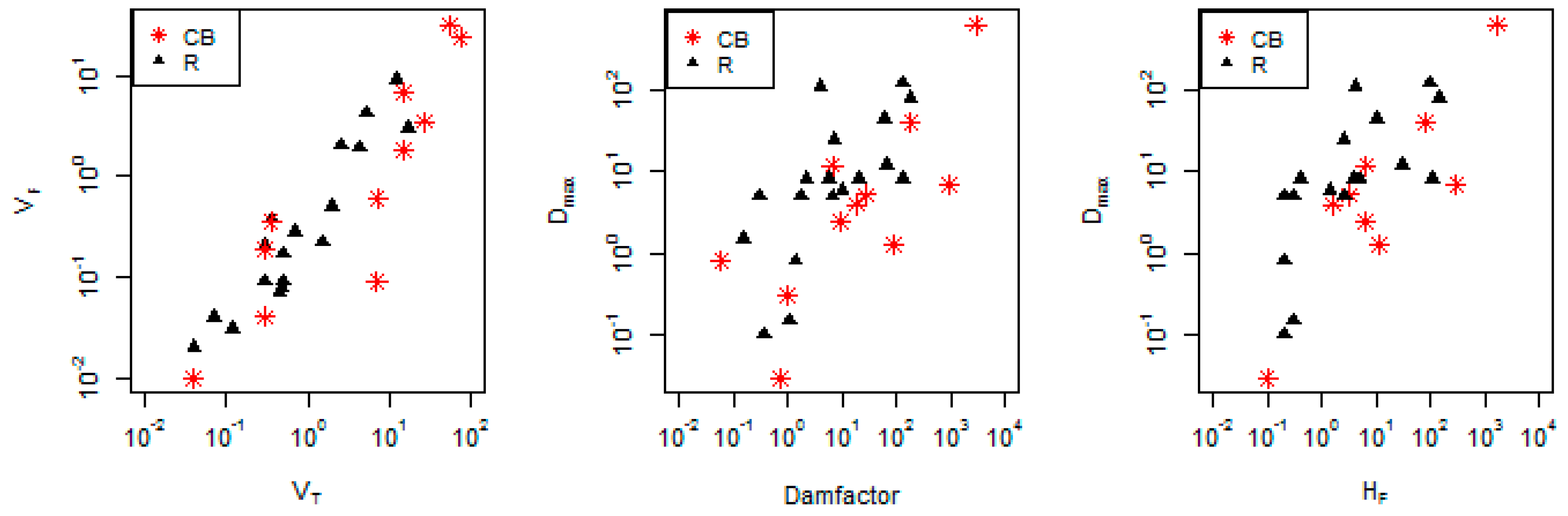
Figure 1 shows the relationships between VF and VT, and Dmax with H × VF (called dam factor in [10]) using the updated dataset (plots in log scale), and DmaX with Hf, (Equation (3)). VF and VT show a linear relationship in the log form, while for Dmax, there is greater dispersion with the dam factor and Hf.
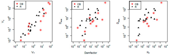
Figure 1.
Left: Relationship between VF and VT in ×106 m3. Center: Dmax in km in relation to the dam factor (H × VF). Right: Dmax in km in relation to Hf (H × (VF/VT) × VF). All plots are in the log-log scale. Note that the Dmax vs. Hf plot is much tighter than the Dmax vs the dam factor plot. CB are added points from Chambers and Bowker [15] and R are from Rico [10].
VF was estimated in the same way as in Rico et al. [10] using the predictor VT with a log-log (power) transformation and the updated data. For the estimation of Dmax three models were considered:
The observed value of VF was used to fit the Dmax regressions.
The goodness of fit of each model was analyzed with residual plots, outlier identification, analysis of influential observations using Cook’s distance, and computing the root mean square error(RMSE) using a 5-fold cross validation (CV). The prediction intervals and probability of occurrence of VF and Dmax in three historical failures was compared across models using the original and the updated datasets.
3. Results and Discussion
3.1. Released Volume of Tailings
The presence of the new data points in the updated dataset has an effect in the uncertainty of VF.1 as seen in the R2, standard error and 5-fold cross validation results in Table 3. In Samarco, 58% of the tailings contained at the Fundão dam were released (P.15 in Table 1), whereas in the incident of the Gypsum tailings dam in Texas only 1.2% of the contained tailings were released (P.17 in Table 1). The Gypsum tailings dam incident (P.17) was not included in the updated regression (Equation (4)) because it was a minor release, different from the characteristics of the rest of the dataset (identified as an outlier with high influence, Table 3), and had a strong effect in the normality of the residuals.
Table 3.
Results for VF.1 with the original Rico dataset (O) and updated (U) datasets (including P.17).
The final regression equation with the updated dataset excluding P.17 is,
R2 = 0.887; standard error: 0.315.
Using Rico’s notation, this may be expressed as . However, since the model is fit in terms of log(VF) it is important to consider the uncertainty of prediction in terms of log(VF), and then transform the prediction intervals to real space to determine the proper uncertainty intervals for VF. Tests for the residuals from the fit provided by Equation (4) indicate that a Gaussian distribution cannot be rejected for the residuals at the 5% level (Shapiro-Wilk test p-value = 0.1161). The prediction intervals are then computed at the desired significance level for log(VF) and then transformed to real space for VF.
Table 4 shows the prediction of VF and 90th prediction interval for Samarco, Mt. Polley and the Gypsum TSF using Equation (4). These cases were selected based on the influence they have in the regression of VF with the updated data (Table 3). The prediction intervals are wider and the predicted mean is larger for Samarco and Mt. Polley when the original dataset is used. In the case of the Gypsum tailings dam, the observed value is not within the prediction interval in neither regression because the volume released was so small and the probability of exceeding it was very high (the same was observed even when that data point was included in the regression).
Table 4.
Predicted and observed VF values in ×106 m3 for select cases (using all the points in the original Rico dataset (O) and updated (U) data sets except P.17 in U).
As mentioned in the introduction, the volume of released tailings will vary greatly depending on the type of failure and the composition of the tailings but for a first estimate of potential damage, the scenarios within the prediction interval are useful to assess a range of potential consequences. The upper prediction interval for VF should be constrained by the total volume of tailings available since in all the cases presented in Table 4, the 95th percentile is more than what is physically possible (more than the total impounded are released). In this case, finding the probability associated with totally emptying the dam would be a better approach for risk estimation. We developed an online pp that has the capability of computing the probability of exceeding a value of VF specified by the user (available at https://columbiawater.shinyapps.io/ShinyappRicoRedo/). In this manner, the uncertainty around VF can be considered when estimating Dmax. The app also provides Q5, Q50 and Q75 of VF. From Table 1, P.10, P.13, P.28, and P.29 were nearly or totally emptied.
3.2. Run-Out Distance (Dmax)
The analysis of Dmax.1 (the original model by Rico et al. [10]) using the updated and original datasets, shows that the uncertainty increases when the new data points are introduced; R2 is reduced and the cross validated error increases (Table 5). The Samarco failure is an influential observation in all the Dmax regressions except for Dmax.3 (Table 5). The distance traveled by the tailings reached 637 km, although more than 90% of the tailings stayed within 120 Km of the dam, the rest were transported in the Doce river all the way to the Atlantic Ocean [15]. The Bonsal TSF (P.7) is also identified as an influential observation (Table 5), this incident had a large Dmax (close to 1 km) compared to the released volume of tailings (the released volume of tailings was approximately 0.01 m3). The failure mode reported at P.7 was overtopping so it is likely that the tailings dam had a large proportion of water at the time of failure. P.12 also appears as an influential observation; in that case the distance traveled by the tailings was only 30 meters, which is small considering the dam height (18 m) and the released volume of tailings (0.038 Mm3).
Table 5.
Results of the fitted models for Dmax.
Based on the results from Table 5 (R2, and 5-fold CV) and the analysis of the residual plots, the best model found was Dmax.3, which uses the new predictor Hf and has the form:
Residual standard error = 0.658. Using Rico’s notation, this may be expressed as
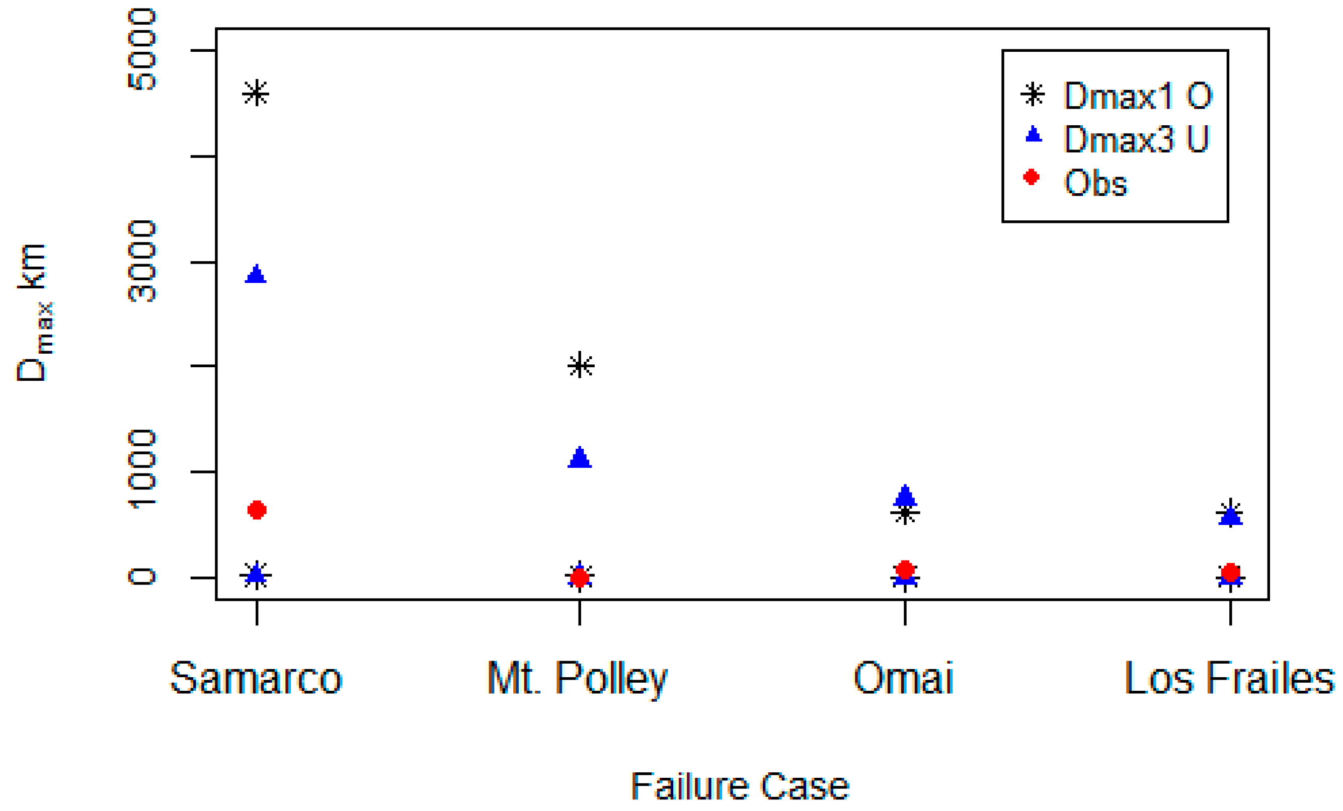
Table 6 includes the results of the prediction and prediction intervals using the original model (Dmax.1) with the original and the updated datasets, and includes the results of Dmax.3 for three of the influential observations. The uncertainty distributions are obtained as before by considering the residuals associated with Equation (5), testing for Gaussian structure (Shapiro-Wilk test p-value = 0.388), and then computing the prediction intervals at the desired significance levels, and transforming them to real space. Figure 2 has examples of the prediction intervals obtained from Dmax.1 O and Dmax.3 U compared to the observations. From the results in Table 6 and Figure 2 is evident that the additional data used to fit the regressions of Dmax dramatically reduces the uncertainty bounds in the prediction of large events such as Samarco and Mt. Polley, although in smaller Dmax events such as Bonsal, Los Frailes or Omai, the uncertainty is similar or it increases. The probability of exceeding the observed run-out distance shown in Table 6 was calculated transforming the observation to the log space, and evaluating its location in the distribution associated to the prediction interval (t distribution). This is exemplified in Figure 3.
Table 6.
Predicted values (in km) using all the data points for training the models (using the observed VF).
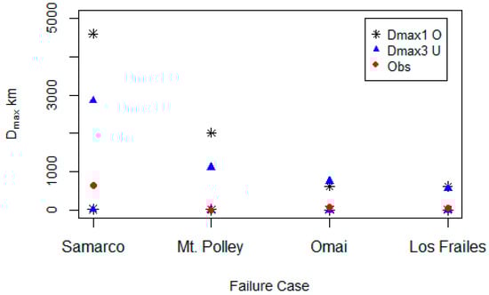
Figure 2.
Examples of prediction intervals from Dmax. 1 O (Rico’s original equation), Dmax.3 U and the observations for Dmax of past failures (obs).
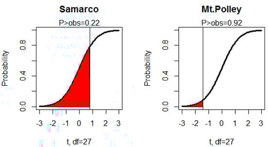
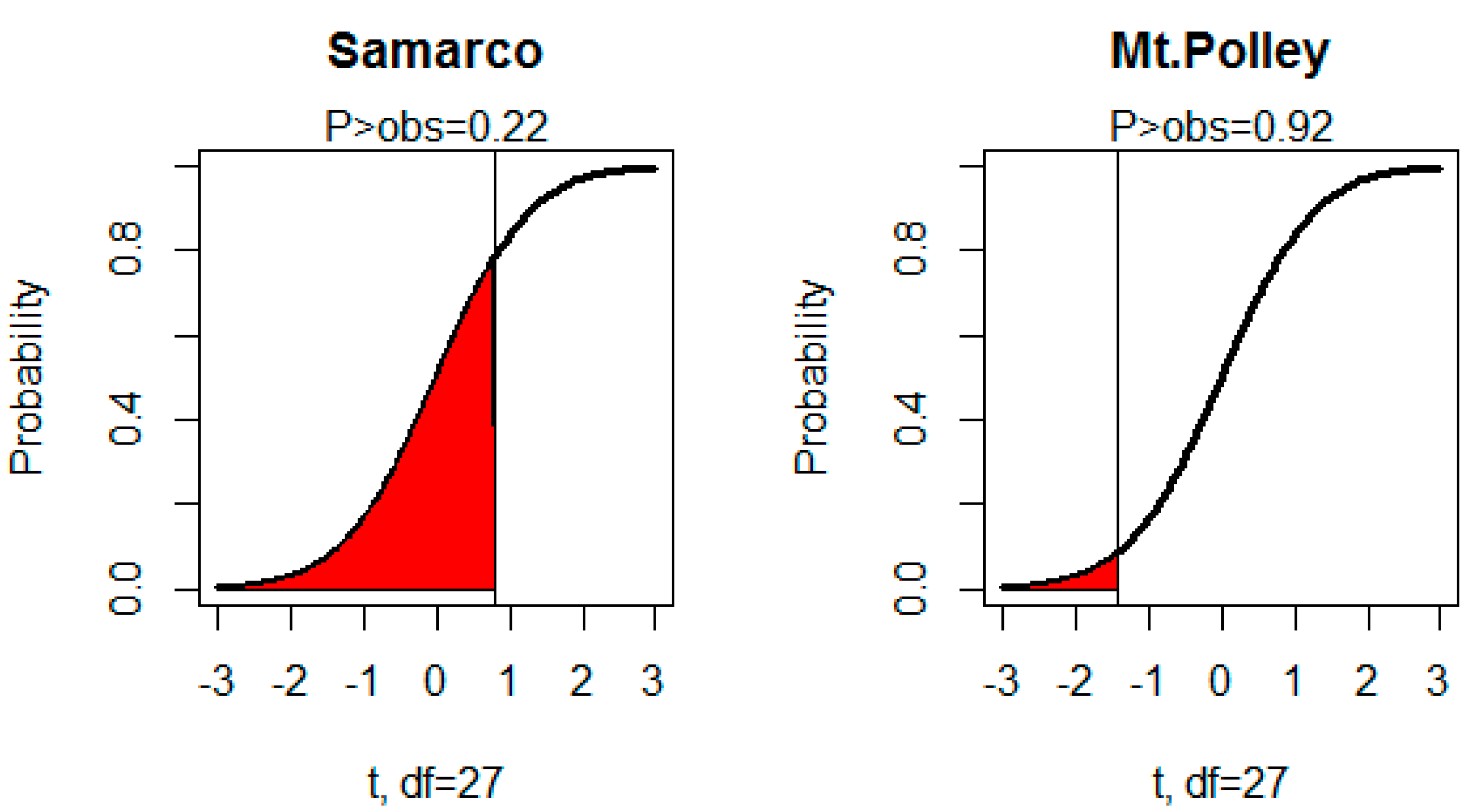
Figure 3.
t distributions showing the probability of exceedance of the Samarco and Mt. Polley observed Dmax and the distributions obtained with model Dmax.3 around the predicted mean value of Dmax in the log space.
The importance of considering the uncertainty distribution around the regression of Dmax, rather than using the conditional mean directly is illustrated by the examples in Table 6. For the Samarco incident, the mean value of the predicted Dmax is 174 km using Dmax.3, while the predicted 5th (95th) percentile is 10 (2933) km. The Dmax reported from the actual failure was 637 km downstream, which based on the uncertainty distribution associated with the regression equation, has a probability of exceedance of approximately 22% using model Dmax.3. In this case the tailings were deposited directly in the Doce River [4], transporting the tailings all the way to the Atlantic Ocean, whereas for other TSF failures an immediate river receptor may not be there, limiting the travel distance. Consequently, if just the conditional mean of the regression equations such as those developed by Rico et al. [10] is used, then one would be rather poorly informed as to the range of potential consequences of a failure. For a probabilistic risk evaluation then, for Samarco, the concern would have been the greater than 600 km impact with a 22% chance rather than the modest 174 km indicated by the regression. It is important to highlight that the observed VF was used to fit all the DmaX regressions but in reality this value might not be known prior to a failure. Therefore, the uncertainty of the estimation of VF from Equation (4) has to also be considered in the predictions of Dmax, which will increase the uncertainty. This is also an issue with Rico’s approach reported in Equations (1) and (2), and it is acknowledged in their paper. In the online app we developed, this is addressed and Dmax can be calculated taking into account the uncertainty around VF in a two-step model.
4. Conclusions
The empirical equations developed by Rico et al. [10] to estimate the volume of tailings released in a tailings dam failure and the run-out distance of the tailings were reviewed. An updated dataset provided information on dam failures that happened after the Rico et al. [10] paper was published and includes cases of dams with larger storage capacity and height than the points in the original dataset. The introduction of the new data points in the regression reduces the uncertainty of the prediction of large failure incidents such as the one occurred in Samarco.
An improved model to estimate the run-out distance is proposed. The model uses the predictor Hf that considers the potential energy associated with the released volume as opposed to the whole tailings impoundment volume. The model proposed has a better linear fit than the original model when using the updated dataset. The updated model to calculate VF is presented in Equation (4), and the new model to estimate Dmax in Equation (5). We recommend using the app we provide which contains the equations (available at https://columbiawater.shinyapps.io/ShinyappRicoRedo/). Since we recommend using the uncertainty distribution for each “prediction” it is easiest for the user to use our web app. As data on other failures becomes available, it can be brought into the app and the model can then be automatically updated.
This paper emphasizes that these are empirical regression equations with significant uncertainty about the mean. Some investigators directly use such regression equations in a deterministic way to specify exposure. However, at site conditions vary significantly (rheology, water content, failure type, etc.), and even with the log-log regressions presented here, there is considerable uncertainty that needs to be quantified. It is important to account for the uncertainty in these estimates to derive a probabilistic measure of risk that also accounts for how well the regression fits in a certain range of values of the predictors.
Acknowledgments
This work was supported by Norges Bank Investment Management. We would like to acknowledge Lindsay Bowker for directing us to the updated dataset of historical tailings dams’ failures used in this paper.
Author Contributions
Paulina Concha gathered and analyzed the data. The conception, design, and writing of the paper were done between Paulina Concha and Upmanu Lall.
Conflicts of Interest
The authors declare no conflict of interest. The founding sponsors had no role in the design of the study; in the collection, analyses, or interpretation of data; in the writing of the manuscript, and in the decision to publish the results.
References
- BHP Billiton Results for The Year Ended 20 June 2016. Available online: http://www.bhp.com/-/media/bhp/documents/investors/news/2016/160816_bhpbillitonresultsyearended30june2016.pdf?la=en (accessed on 1 July 2017).
- Form 20-F, Annual Report Pursuant to Section 12 or 15(d) of the Securities Exchange Act of 1934. Available online: http://www.vale.com/EN/investors/information-market/annual-reports/20f/20FDocs/Vale_20-F_FY2016_-_i.pdf (accessed on 1 July 2017).
- Renova Foundation Update. Available online: http://www.bhp.com/-/media/documents/media/reports-and-presentations/2017/170607_renovafoundationupdate.pdf (accessed on 1 June 2017).
- Fernandes, G.W.; Goulart, F.F.; Ranieri, B.D.; Coelho, M.S.; Dalesf, K.; Boesche, N.; Bustamante, M.; Carvalho, F.A.; Carvalho, D.C.; Dirzo, R.; et al. Deep into the mud: Ecological and socio-economic impacts of the dam breach in Mariana, Brazil. Nat. Conserv. 2016, 14, 35–45. [Google Scholar] [CrossRef]
- Design of Tailings Dams and Impoundments. Available online: http://www.infomine.com/library/publications/docs/Davies2002b.pdf (accessed on 1 April 2017).
- Caldwell, J.A.; Van Zyl, D. Thirty years of tailings history from tailings & mine waste. In Proceedings of the 15th International Conference on Tailings and Mine Waste, Vancouver, BC, Canada, November 2011. [Google Scholar]
- Morgenstern, N.R. Improving the safety of mine waste impoundments. In Tailings and Mine Waste 2010; CRC Press: Vail, CO, USA, 2010; pp. 3–10. [Google Scholar]
- Strachan, C.; Caldwell, J. New directions in tailings management. In Tailings and Mine Waste 2010; CRC Press: Vail, CO, USA, 2010; pp. 41–48. [Google Scholar]
- Martin, V.; Akkerman, A. Challenges with conducting tailings dam breach studies. In Proceedings of the 85th Annual Meeting of International Commission on Large Dams, Prague, Czech Republic, July 2017. [Google Scholar]
- Rico, M.; Benito, G.; Diez-Herrero, A. Floods from tailings dam failures. J. Hazard. Mater. 2008, 154, 79–87. [Google Scholar] [CrossRef] [PubMed]
- Pierce, M.W.; Thornton, C.I.; Abt, S.R. Predicting peak outflow from breached embankment dams. J. Hydraul. Eng. 2010, 15, 338–349. [Google Scholar] [CrossRef]
- MacDonald, T.; Langridge-Monopolis, J. Breaching characteristics of dam failures. J. Hydraul. Eng. 1984, 110, 567–586. [Google Scholar] [CrossRef]
- Álvarez, M.; Puertas, J.; Peña, E.; Bermúdez, M. Two-dimensional dam-break flood analysis in data-scarce regions: The case study of Chipembe dam, Mozambique. Water 2017, 9, 432. [Google Scholar] [CrossRef]
- Cannata, M.; Marzocchi, R. Two-dimensional dam break flooding simulation: A GIS-embedded approach. Nat. Hazards 2012, 61, 1143–1159. [Google Scholar] [CrossRef]
- TSF Failures 1915–2017 as of 16 August 2017. Available online: http://www.csp2.org/tsf-failures-1915-2017 (accessed on October 2017).
- Blight, G.E.; Robinson, M.G.; Diering, J.A.C. The flow of slurry from a breached tailings dam. J. South. Afr. Inst. Min. Metall. 1981, 1, 1–10. [Google Scholar]
- Tailings Dams Risk of Dangerous Occurrences. Lessons Learnt from Practical Experiences. Available online: http://www.unep.fr/shared/publications/pdf/2891-TailingsDams.pdf (accessed on 11 January 2018).
- Chronologies of Major Tailings Dams Failures. Available online: http://www.patagoniaalliance.org/swp-content/uploads/2014/09/Chronology-of-major-tailings-dam-failures.pdf (accessed on 4 September 2014).
- Fonseca do Carmo, F.; Kamino, L.H.Y.; Tobias, R.; de Campos, I.C.; Fonseca do Carmo, F.; Silvino, G.; de Castro, K.J.S.X.; Mateus Leite, M.; Rodrigues, N.U.A.; et al. Fundão tailings dam failures: The environment tragedy of the largest technological disaster of Brazilian mining in global context. Perspect. Ecol. Conserv. 2017, 15, 145–151. [Google Scholar] [CrossRef]
- Los Frailes Tailings Incident, Mining & Environment Research Network. Available online: http://www.pebblescience.org/pdfs/LosFrailes.pdf (accessed on 25 April 1998).
- La Catástrofe de Aznalcóllar, X Aniversario: ¿Una Lección Aprendida? Available online: http://assets.wwf.es/downloads/_informe_2008.pdf (accessed on 1 April 2008).
- Van Niekerk, H.J.; Viljoen, M.J. Causes and consequences of the Merriespruit and other tailings-dam failures. L. Degrad. Dev. 2005, 16, 201–212. [Google Scholar] [CrossRef]
- Feng, C.; Wang, H.; Lu, N. Log-transformation and its implications for data analysis. Shanghai Arch. Psychiatry 2014, 26, 105–109. [Google Scholar] [PubMed]
© 2018 by the authors. Licensee MDPI, Basel, Switzerland. This article is an open access article distributed under the terms and conditions of the Creative Commons Attribution (CC BY) license (http://creativecommons.org/licenses/by/4.0/).