Simple Summary
The objective of this study was to evaluate the genetic background and inbreeding depression in the Mexican Romosinuano cattle using pedigree and genomic information. Inbreeding was estimated using pedigree () and genomic information based on the genomic relationship matrix () and runs of homozygosity (). Linkage disequilibrium () was evaluated using the correlation between pairs of loci, and the effective population size () was calculated based on and pedigree information. The pedigree file consisted of 4875 animals; 71 had genotypes. decreased with the increase in distance between markers, and estimated using genomic information decreased from 610 to 72 animals (from 109 to 1 generation ago), the estimated using pedigree information was 86.44. The number of runs of homozygosity per animal ranged between 18 and 102 segments with an average of 55. The average inbreeding was 2.98 ± 2.81, 2.98 ± 4.01, and 7.28 ± 3.68% for , , and , respectively. A 1% increase in inbreeding decreased birth weight by 0.103 kg and weaning weight by 0.685 kg. A strategy such as optimum genetic contributions to maximize selection response and manage the long-term genetic variability and inbreeding could lead to sustainable breeding programs for the Mexican Romosinuano cattle breed.
Abstract
The ultimate goal of genetic selection is to improve genetic progress by increasing favorable alleles in the population. However, with selection, homozygosity, and potentially harmful recessive alleles can accumulate, deteriorating genetic variability and hampering continued genetic progress. Such potential adverse side effects of selection are of particular interest in populations with a small effective population size like the Romosinuano beef cattle in Mexico. The objective of this study was to evaluate the genetic background and inbreeding depression in Mexican Romosinuano cattle using pedigree and genomic information. Inbreeding was estimated using pedigree () and genomic information based on the genomic relationship matrix () and runs of homozygosity () of different length classes. Linkage disequilibrium () was evaluated using the correlation between pairs of loci, and the effective population size () was calculated based on and pedigree information. The pedigree file consisted of 4875 animals born between 1950 and 2019, of which 71 had genotypes. decreased with the increase in distance between markers, and estimated using genomic information decreased from 610 to 72 animals (from 109 to 1 generation ago), the estimated using pedigree information was 86.44. The reduction in effective population size implies the existence of genetic bottlenecks and the decline of genetic diversity due to the intensive use of few individuals as parents of the next generations. The number of runs of homozygosity per animal ranged between 18 and 102 segments with an average of 55. The shortest and longest segments were 1.0 and 36.0 Mb long, respectively, reflecting ancient and recent inbreeding. The average inbreeding was 2.98 ± 2.81, 2.98 ± 4.01, and 7.28 ± 3.68% for , , and , respectively. The correlation between and was −0.25, and the correlations among and of different length classes were low (from 0.16 to 0.31). The correlations between and of different length classes were moderate (from 0.44 to 0.58), indicating better agreement. A 1% increase in population inbreeding decreased birth weight by 0.103 kg and weaning weight by 0.685 kg. A strategy such as optimum genetic contributions to maximize selection response and manage the long-term genetic variability and inbreeding could lead to more sustainable breeding programs for the Mexican Romosinuano beef cattle breed.
1. Introduction
Creole cattle breeds in the American continent originated from the Iberian Peninsula cattle five centuries ago. One of them is the Romosinuano breed, developed from isolation and adaptation to harsh environments in Colombia and has spread mainly to Costa Rica, the United States of America, Venezuela, and Mexico [1]. Over time, the Creole cattle breeds have adapted to adverse tropical conditions; therefore, genes associated with extreme environments and parasite resistance have been selected by natural selection. In Mexico, the national herd of Romosinuano beef cattle was established with the use of germplasm from Costa Rica (Turrialba) and later from the United States (Florida State University) [1].
The Romosinuano breed captured the attention of Mexican beef producers because animals of this breed have good growth performance and meat quality, high fertility, and the ability to adapt to hot and humid conditions and large parasite infestation (e.g., ticks; De Alba [1]). In 1998, local breeders established the “Asociación Mexicana de Criadores de Ganado Romosinuano y Lechero Tropical” (AMCROLET; De Alba [1]). With the creation of AMCROLET, performance information started being recorded to establish a genetic evaluation to improve birth weight and weaning weights [2].
The national herd of Romosinuano beef cattle in Mexico is currently located in tropical areas in the Mexican states of Campeche, Michoacán, Tabasco, Tamaulipas, and Veracruz [2], and the existence of a large number of multiplier herds indicates that the national population is growing [3].
Núñez-Domínguez et al. [3] characterized the population structure and evaluated the genetic variability of the Mexican Romosinuano population with pedigree data and concluded that the genetic diversity has been decreasing, mainly due to random loss of genes. Hence, it is important to reduce such losses of genetic diversity to ensure the breeding program’s sustainability and the breed itself in Mexico. The accumulation of deleterious alleles due to the increase in inbreeding can reduce livestock’s performance and fitness. This reduction is referred to as inbreeding depression, and the study thereof is also crucial in populations with small effective population size.
The accuracy of genetic parameters and inbreeding coefficients estimated using pedigree information heavily depends on its integrity. For instance, pedigree completeness has a substantial effect on estimating the inbreeding coefficient because the probability of finding common ancestors increases with the degree of pedigree completeness [4] Furthermore, missing pedigrees lead to assumed relationships of zero among animals with and without pedigree information, which may not be true. To alleviate this problem, VanRaden [5] presented a method that substitutes these zero relationships by the average relationships among animals born in specific years. In the study by Núñez-Domínguez et al. [3] on the Romosinuano breed in Mexico, the pedigree completeness was low; for example, going back three generations, the pedigree completeness was only 65.2%. The authors highlighted the necessity of more and accurate data recording as well as better estimates of demographic and genetic parameters.
Recently, the development of molecular techniques and the availability of genomic information, such as high-density single-nucleotide polymorphisms (SNP) panels, have made it possible to expand genetic diversity studies in cattle populations. To explore the genetic diversity across the genome and develop tools to design sustainable and more appropriate breeding programs, the AMCROLET has recently obtained the genotypes of 71 animals (54 K SNP markers). The first objective of the present study was to evaluate the genetic background of the Romosinuano beef cattle breed in Mexico, using different approaches: (i) pedigree analysis; (ii); inbreeding coefficients estimated by pedigree and genomic information; (iii) analysis of linkage disequilibrium and effective population size. A second objective was to assess the effect of inbreeding on birth weight and weaning weight traits.
2. Materials and Methods
2.1. Pedigree Genotypes and Phenotypes
The AMCROLET provided the genealogical information, phenotypes, and genotypes used in this research study through the performance-recorded database for the Romosinuano beef cattle breed. The pedigree file consisted of 4875 animals, progeny of 219 sires and 1685 dams, born between 1950 and 2019.
Seventy-one animals were genotyped with the medium-density Affymetrix chip (54 K SNP markers). The genotyped animals were 22 males and 49 females born between 2003 and 2018 and were selected among the alive animals in the population-based on their contribution to the population (i.e., animals with more progeny were selected). The average number of progeny in the group of genotyped animals was 3.7 for males and 1.7 for females. Quality control on animals and markers was performed using PLINK software version 1.90 [6], according to the following parameters: minimum call rate equal to 95%, minor allele frequency of each marker greater than 1%, the threshold to exclude markers that deviate from Hardy–Weinberg equilibrium was a p-value set to 10−6. SNP mapped on sexual chromosomes or not mapped on the Bos taurus autosome (BTA) 3.1.1 release were also discarded. Markers mapped on sexual chromosomes were discarded due to big differences between males and females allosomes. Animals and markers that failed these quality control criteria were removed. All the animals were retained; a total of 30,571 SNP markers mapped on 29 autosomal chromosomes were retained for further analyses.
The phenotypic information included a total of 1328 birth weight phenotypes [mean (SD); 27.13 (4.88) kg], and 690 weaning weight phenotypes [mean (SD); 144.28 (27.92) kg]. Animals with phenotypes were born between 2001 and 2019 and had both sire and dam known. The number of genotyped animals with phenotypes were 51 for birth weight and 37 for weaning weight.
2.2. Pedigree Analyses
The pedigree analyses were performed using the Endog software version 4.8 [7]. The following parameters were calculated: pedigree-based inbreeding coefficient (), relatedness coefficient (), generation intervals, equivalent complete generations, realized effective population size, probabilities of gene origin, and the number of progeny per sire and dam. The pedigree analysis was done for the whole population (4875 animals), and a reference population consisted of 1058 animals born between 2013 and 2019. The reference population represents the animals born in the last generation of the population. It was defined based on the generation interval of this population estimated by Núñez-Domínguez et al. [3], which was ~7 years in this population.
2.2.1. Inbreeding and Relatedness Coefficient
The pedigree-based inbreeding coefficient for each animal represents the probability that two alleles at any locus are identical by descent [8], and it was computed using the algorithm of Meuwissen and Luo [9]. Each animal’s relatedness coefficient was computed as the probability that an allele selected randomly from the entire population included in the pedigree belonged to a particular animal. The can be interpreted as the animal’s representation in the context of the entire pedigree, without knowledge of its pedigree [10].
2.2.2. Equivalent Complete Generations
Equivalent complete generations assessed the completeness of the pedigree. Equivalent complete generations for an individual ( were calculated according to Maignel et al. [11] as follows:
where is the number of generations separating the individual from each known ancestor in the pedigree. The percentage of known ancestors during the last ten generations was calculated. The pedigree completeness index () was generated for each generation. The represents the mean proportion of ancestors known in each ancestral generation and was computed as the proportion of known ancestors in each ascending generation. For example, the second generation for a given animal was assigned completeness measure 1.0 if all four grandparents were known, 0.75 if three were known, and so on [12].
2.2.3. Generation Interval
The generation interval () was calculated as the parents’ average age at their progeny’s birth time kept for reproduction. It was calculated across the four genetic pathways, sire of sire (), sire of dam (), dam of sire (), and dam of dam (). The average generation interval was computed as follows:
2.2.4. Realized Effective Population Size
The effective population size is the size of an ideal population, characterized by equal sex ratio, absence of mutation, migration and selection, which has the same inbreeding rate as the real population under study. The realized effective population size () was estimated based on the individual increase in inbreeding. The coefficients of individual increase in inbreeding () were computed according to the method described by Gutiérrez et al. [13] and modified by Gutiérrez et al. [14], using the following formula:
where and are the inbreeding coefficient and the equivalent complete generations for individual , respectively. The coefficients of individual increase in inbreeding were averaged, and the realized effective population size was estimated as:
2.2.5. Probabilities of Gene Origin
Changes in the genetic diversity and population structure, such as recent bottlenecks, were assessed based on the probability of gene origin. Two parameters on the probability of gene origin, including the effective number of founders and ancestors, were estimated. The effective number of founders () denotes the number of equally contributing founders that would result in the same level of genetic diversity in the current population, and it was estimated according to Lacy [15]:
where is the expected proportional genetic contribution of founder ; computed as the average relationship of the respective founder to each animal in the population, and is the total number of founders.
The effective number of ancestors () measures the minimum number of ancestors (not necessarily founders) explaining the complete genetic diversity of the current population, and it was computed according to Boichard et al. [10]:
where is the marginal contribution of each ancestor, which is the contribution made by an ancestor not explained by a previously chosen ancestor, and is the total number of ancestors.
The is lower than the , and the comparison of both numbers can be used to evaluate the impact of bottlenecks that may have occurred from the founders to the present population [10]; the lower the / ratio, the more stringent the bottlenecks were.
2.3. Genomic Analyses
2.3.1. Inbreeding Coefficients
Individual genomic inbreeding coefficients were calculated by two methods. In the first method, genomic inbreeding coefficients were obtained from the genomic relationship matrix (). The were calculated by subtracting one from the diagonal elements of the genomic relationship matrix (), built according to VanRaden [16] as follows, and using the BLUPF90 program [17]:
where is the matrix of centered gene content, and is the minor allele frequency of . The is sensitive to the allele frequencies used to compute the genomic relationship matrix [18,19]. Therefore, in this research study, allelic frequencies were fixed to 0.5 instead of calculated from the current genotypes because of the small number of genotyped animals.
In the second method, runs of homozygosity () were used to compute individual genomic inbreeding coefficients. Consecutive were computed through the algorithm implemented in the R package “DetectRuns” [20]. Runs of homozygosity were defined as 15 consecutive homozygous SNP covering a least 1 Mb in length. To be more conservative, heterozygotes and missing markers were not allowed into . The maximum distance between consecutive markers was 1 Mb. Average length () was computed for each animal, and according to their length, were grouped into five different classes: 1–2 Mb, 2–4 Mb, 4–8 Mb, 8–16 Mb, >16 Mb [21]. The number of () and the sum of all the () per individual were also computed. Specific , i.e., homozygous regions starting and ending precisely at the same positions within the chromosome, were also computed [22]; these segments can be found in one or more animals. Individual -based inbreeding coefficients were estimated at the genome-wide level () and by chromosome () as follows:
where is the total length of all the detected in the animal’s autosomes, is the total length of the autosomal genome; calculated as the sum of the lengths of the 29 autosomal chromosomes (2507.77 Mb), is the total length of the chromosome, calculated as the length between the position of the first and the last SNP in the chromosome. The length of the chromosomes ranged from 42.90 Mb (BTA25) to 158.03 Mb (BTA1).
2.3.2. Linkage Disequilibrium and Effective Population Size
The historical trajectory of effective population size was estimated through linkage disequilibrium () using the SNeP V1.1 software [23]. The was evaluated using the squared Pearson’s product-moment correlation coefficient between pairs of loci ( for unphased data as proposed by Barbato et al. [23] as follows:
where and are two separate loci, and are the mean genotype frequencies for the first and second locus, respectively, is the genotype of individual at the first locus, and is the genotype of individual at the second locus.
The trajectory of effective population size () was also estimated using the SNeP V1.1 software. This software estimates the historical based on the relationship among , , and (recombination rate), applying the following formula proposed by Corbin et al. [24]:
where is the effective population size generations ago, which is equivalent to , presented by Hayes et al. [25]; is a mapping function related to the recombination rate; is the adjusted for sampling bias. In the sampling bias adjustment (due to small sample size ()), the input parameter is in , in this research study we used for unphased data. Because we studied long distances (>100 Mb) between SNP to estimate in recent generations, we applied an adjustment to the recombination rate through the mapping function developed by Sved and Feldman [26] to translate the estimated linkage distance () into the recombination rate: . The value of was 2 to correct for the occurrence of mutations as proposed by Tenesa et al. [27]. Other included options related to the minimum and maximum distance between SNP were -mindist (100 kb) and -maxdist (35,000 kb), respectively. Short distances allowed the estimation of in distant generations, whereas longer distances allowed the estimation of in recent generations.
2.4. Selection Signatures
Genomic regions under selection can be defined as highly homozygous ( islands) and heterozygous ( islands) regions [28]. The and islands were obtained based on the SNP frequency (times that each SNP was detected in a run divided by the number of animals) within and , respectively. The SNP from the top 0.01% (99.9 percentile was defined as a threshold) of the distribution were selected to define a region as an “island”.
The runs of heterozygosity were obtained using the consecutive method in the R package “DetectRuns” [20]. The were defined as 15 consecutive heterozygous SNP covering at least 250 kb in length. Inside the , the allowed number of homozygous and missing markers was three and two, respectively. The maximum distance between consecutive markers was set to 1 Mb.
Identification of the genes within the highly homozygous and heterozygous genomic regions detected was obtained from the Genome Data Viewer tool provided by NCBI (https://www.ncbi.nlm.nih.gov/genome/gdv/browser/genome/?id=GCF_002263795.1). The Bos taurus genome assembly ARS-UCD1.2 was used as a reference.
2.5. Inbreeding Depression Analysis
Quality control on the phenotypes considered: (1) for both traits, observations outside of the range mean 3 standard deviations were discarded; (2) weaning weight phenotypes were adjusted to 240 d of age; animals with phenotypes recorded outside of the range 240 45 d of age were removed.
Inbreeding depression was estimated for birth weight and weaning weight by regressing the phenotypes on inbreeding coefficients. The inbreeding depression was estimated in two groups of animals: (1) in all the animals with phenotypes and (2) in animals with phenotypes and genotypes. Pedigree-based inbreeding coefficients were used in both cases, while the inbreeding coefficients obtained by genomic analyses were used only in the second scenario. The traits were analyzed separately using the following linear model:
where, is the phenotype of animal belonging to the sex class , born in the year , is the overall intercept, is the regression coefficient on the individual level of pedigree () or genomic () inbreeding, and is the residual term assumed to be normally distributed.
All regression analyses and summary statistics were carried out using the R software [29].
3. Results and Discussion
3.1. Pedigree Analysis
In the population of Mexican Romosinuano beef cattle, the pedigree had 27% and 35% of missing information for sire and dam pathways, respectively. Therefore, it is necessary to improve the pedigree recording at the population level, especially from the maternal side. On average, the number of progeny was 16.24 ± 25.06 (maximum 144) per sire and 1.84 ± 1.72 (maximum 12) per dam. A total of 361 full sibs were found from the pedigree, representing 8% of all animals.
3.1.1. Inbreeding and Relatedness Coefficient
The average was 1.52% in the total population and 2.63% in the reference population. The percentage of inbred animals was 32.4% in the total population and 54.6% in the reference population. The average was 4.69% in the inbred animals in the total population and 4.81% in the reference population. The estimations in the total and reference populations suggest that the inbreeding level is low in the Mexican Romosinuano. However, underestimation due to the shallow and missing pedigrees must be recognized. Indeed, Barczak et al. [30] reported that a pedigree with many missing ancestors could lead to underestimated inbreeding coefficients. In the reference population, the percentage of inbred animals and the were greater than that of the total population, indicating loss of genetic diversity that could adversely impact the animals’ performance adversely.
The evolution of and over time is shown in Figure 1A. The relatedness coefficient is inversely related to genetic diversity and can be used as an indicator of inbreeding in the long term. When is greater than in the population, the mating between relatives is more frequent, and in general, when tends to approach zero, the genetic diversity increases. Therefore, when selecting top animals, it is important to consider the animals with lower values. The estimated in total and reference populations was 3.13 and 4.32%, respectively. The was always greater than , indicating that the frequency of mating between related animals was greater than the frequency of mating between unrelated individuals. It is also important to highlight that during the last 20 years, and presented an increasing trend (Figure 1A). Thus, some efforts should be made to avoid genetic diversity erosion.
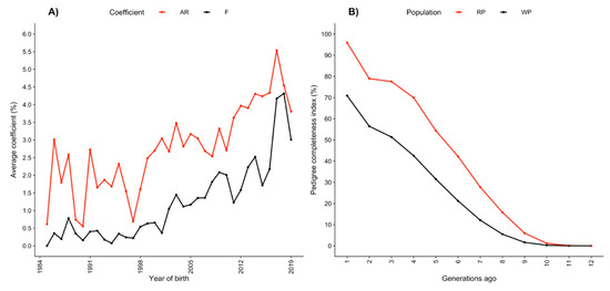
Figure 1.
(A) Evolution of the average pedigree-based inbreeding () and relatedness () coefficients from 1984 to 2019; (B) pedigree completeness index in the whole (WP) and reference (RF) populations.
3.1.2. Equivalent Complete Generations
The average equivalent complete generations were 2.9 in the total population and 4.7 in the reference population. The pedigree completeness index one generation ago was 70.9 and 95.9% in the total and reference populations, respectively. Tracing back five generations, the pedigree completeness index decreased to 31.5% in the total population and 54.3% in the reference population (Figure 1B). The pedigree completeness index is an important indicator of the quality because it represents the harmonic mean of the parental genetic contributions, and it is zero if any parent is unknown regardless of how deep and complete the pedigree of the other parent is. The improvement in the pedigree completeness index seen at recent generations in the Mexican Romosinuano beef cattle population (Figure 1B) represents recent efforts that were put in place to improve the pedigree recording, and this strategy should continue.
3.1.3. Generation Interval
The generation intervals computed using the four pathways of selection are presented in Table 1. The average generation intervals for the total and the reference populations were similar, with values of 6.25 and 6.52 y, respectively.

Table 1.
Estimates (±SE) of generation interval (GI) for the four selection paths in Mexican Romosinuano beef cattle.
3.1.4. Realized Effective Population Size
The realized effective population size based on the individual increase in was 86.44 14.69, and the individual increase in was 0.578%. The is above the threshold of 50 recommended to maintain the population’s genetic diversity at an acceptable level [31].
3.1.5. Probabilities of Gene Origin
The was 71 and 75, while the was 31 and 30, in the total and reference populations, respectively. A total of 10 and 11 ancestors explained 50% of the genetic diversity in the total and reference populations, respectively. The / ratio was 0.44 in the total population, and it was 0.40 in the reference population, indicating the existence of genetic bottlenecks and loss of genetic diversity in the Mexican Romosinuano beef cattle population. The genetic bottlenecks were narrower in recent years, which agrees with a recent steeper increase in (Figure 1A).
Ramírez-Valverde et al. [32] studied the genetic diversity using pedigree data in six Mexican beef cattle populations of cosmopolitan breeds and reported similar parameters for some breeds, compared to the Mexican Romosinuano beef cattle population presented here. In their study, the progeny number per sire and dam ranged from 6 to 31 and from 1.8 to 2.7, respectively. The authors reported ranging from 0.9 to 4.2%, and from 0.3 to 6.5%, with equivalent complete generations varying from 2.03 to 7.51, generation interval from 5.1 to 7.2 y, and the effective population size from 24 to 192.
Based on the pedigree analysis, the in the Mexican Romosinuano beef cattle population seems to be low. However, an increasing trend was observed, especially in recent years. Overall, the pedigree completeness index was low, with evident improvements in recent years. The generation interval was 6.52 years in the more recent generation, and this value is similar to other beef cattle populations Ramírez-Valverde et al. [32]. The effective population size (86.44) was close to the recommended minimum (50) to maintain genetic diversity at acceptable levels. Finally, genetic bottlenecks were present and narrower in the last generation.
3.2. Genomic Analyses
3.2.1. Inbreeding Coefficients
Inbreeding in itself is neither good nor bad because it reflects homozygosity accumulation. In fact, the primary objective of genetic selection is to increase the frequency of favorable variants, and it can happen in homozygous or heterozygous genotypes. The inbreeding coefficient cannot differentiate between the accumulation of homozygosity of favorable alleles and the accumulation of homozygosity for neutral or deleterious alleles; therefore, it is an imperfect metric of the recessive load of an individual [33].
One way to better understand this situation is by looking at the inbreeding age, measured through the length of segments. This is possible because haplotypes are broken by recombination over time; therefore, short segments were more likely to originate from a more distant origin (i.e., in old generations; ancient inbreeding) [34,35]. On the other hand, recent inbreeding produces long segments with deleterious variants segregating for less time and not still filtered out by purging events yet [33]. Thus, long (recent inbreeding) segments are a better metric of the recessive load of a given individual [36].
Summary statistics of identified across different length classes are reported in Table 2. Across all genotyped animals, a total of 3943 were found; the 1–2 Mb class was the most abundant, accounting for 48.4% of total regions. Only 48 were detected in the upper length class (>16 Mb), and these long regions were identified in 27 different animals; one of these animals showed six long regions and was the animal with the greatest (20.74%). The additive relationship between the parents of this cow was 13.3%, and they shared eight common ancestors across five generations in the pedigree. Of those eight commons ancestors, three of them were part of the group of the 10 ancestors, explaining 50% of the genetic variability in the population. Altogether, these three ancestors explained 25% of the genetic variation in the population. The of this cow was 17.34%, and it had the greatest among the group of genotyped animals. However, the of the cow was not the largest among all the genotyped animals. In fact, the was 6.66%, which is considerably lower than the other inbreeding estimates. This highlights the value of genomic information as a more accurate source of information.
Table 2.
Number, mean length, and number of single-nucleotide polymorphisms (SNP) of runs of homozygosity in different length classes.
The shortest and the longest segments were 1.0 and 36.0 Mb, respectively. The greatest number of per chromosome was found on BTA1 (321), whereas the lowest number was found on BTA28 (50). At the genome-wide level, a large proportion of in all autosomes was in the shortest class (<2 Mb).
Although recent inbreeding is a useful measure to evaluate recessive load, the separation between ancient and recent inbreeding is still an active research topic and remains unclear. Maltecca et al. [33] reported that inbreeding depression was greater for more recent inbreeding than older inbreeding in a Holstein population. Using also Holstein cattle data, Makanjuola et al. [37] carried out a study splitting inbreeding into age classes and concluded that recent inbreeding had more detrimental effects, whereas ancient inbreeding caused even favorable effects. These authors reported a loss of −1.56 kg in 305-d protein yield associated with an increase of 1% in recent inbreeding ( > 4 Mb). Conversely, a gain of 1.33 kg in the same trait was associated with an increase of 1% in ancient inbreeding ( < 4 Mb). A recent research study conducted in beef cattle by Sumreddee et al. [38] demonstrated that although the recessive load is expected to be larger in longer segments, short segments (<5 Mb) can still harbor some deleterious mutations with substantial joint effects on some traits.
In the Mexican Romosinuano beef cattle population, 23.8% of the segments were >4 Mb (Table 2) and potentially represented the recessive load in this population. However, it is important to recognize the small sample size and the necessity to expand the study. More genotyped animals are required to conduct a more comprehensive investigation of regions in this breed.
The average length (, 3.29 ± 3.19 Mb) found in this study was slightly greater than values reported for other small cattle populations but smaller than values estimated in cosmopolitan breeds. Cesarani et al. [39], using the same settings (i.e., minimum 15 SNP, 1 Mb of minimum length and 0 missing and heterozygotes allowed), reported the mean lengths of 2.3 ± 1.8, 2.6 ± 2.3, and 2.4 ± 2.0 Mb for Modicana, Sardo-Bruna, and Sardo-Modicana breeds, respectively. Marras et al. [40] reported values of 3.9 and 3.6 for Brown Swiss and Holstein. The same authors reported an of 1.9 (i.e., almost half of the values found in this study) for the Piedmontese cattle breed. The observed in this study was relatively smaller than that of an inbred line of the Hereford cattle population (6.83 ± 4.45 Mb), as reported by Sumreddee et al. [19].
The length of is a crucial parameter because it is associated with inbreeding events. Long can be found when the mating between relatives occurred recently, whereas short are signs of past events [41]. Gibson et al. [42] and Bosse et al. [43] reported that long homozygote segments are likely to be identical by descent. The results in the present study indicate that the majority of autozygous () segments (1–2 Mb class) identified in this population originated approximately 25 to 50 generations ago, assuming 1 cM equals 1 Mb [44].
On average, 53.97 ± 17.15 were found per animal, with this value ranging from 18 to 102. This value is lower than those reported in the literature for cosmopolitan breeds; Marras et al. [40] found 81.7 per animal in Holstein, whereas Ferencakovic et al. [45] reported 98.9 ± 10.2 per animal in Brown Swiss. However, the per animal presented in this study is greater than the values reported for small populations, such as Polish Red (46.4 ± 9.8; Szmatoła et al. [46]). A similar value (54.0 ± 7.2) was estimated for the Piedmontese cattle breed by Marras et al. [40].
The average total length per animal () was 180.45 ± 92.40 Mb. Compared to found in other studies with cosmopolitan breeds, the found in the present study had an intermediate value. For instance, Szmatoła et al. [46] reported of 290.6 ± 67.2, 142.8 ± 67.4, and 180.5 ± 79.9 Mb for Holstein, Polish Red, and Limousin, respectively. Larger per animal were reported in the literature for Brow Swiss (371 Mb) and Holstein (297 Mb) by Marras et al. [40]. The same authors reported smaller values for the Piedmontese cattle (106 Mb).
In general, animals with a larger number tend to have a greater total length of segments regardless of the length of single regions (Figure 2). The correlation between the number of identified and the total length was 0.9, meaning that the more regions, the larger is the total length. A Similar result (correlation = 0.78) was recently published by Cesarani et al. [39] in European Simmental bulls.
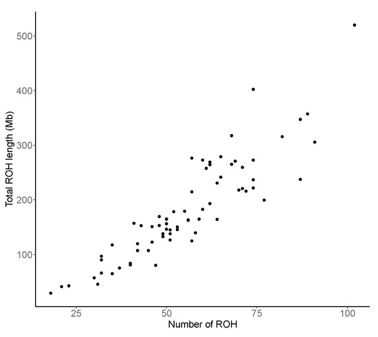
Figure 2.
Relationship between the number of runs of homozygosity (ROH) found in each individual and their total length (Mb).
A total of 319 regions were shared (specific ) by at least two animals (Figure 3A). The most shared region was found in nine animals on chromosome 1, located between 0.13 and 2.36 Mb. The similarity among animals in this region was also confirmed by the plot of stacked runs (Figure 3B).
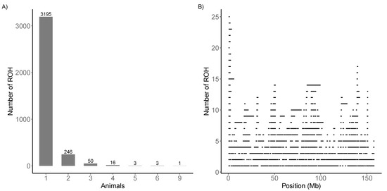
Figure 3.
(A) Specific runs of homozygosity (ROH) distribution. (B) Stacked runs in chromosome 1.
Inbreeding coefficients based on pedigree and genomic information for the 71 genotyped animals are shown in Table 3. Considering all detected (i.e., >1 Mb), the average was 7.28%, and it decreased as the minimum length of increased. This result reflects a decreased number of identified as shorter segments were excluded when longer classes were considered. The average was 1.44% considering the >16 Mb class (Table 3), and this can be attributed to the fact that only a few segments larger than 16 Mb were found. The number of inbred animals in the other classes varied. The total number of inbred animals was 71 for > 1 Mb or > 2 Mb, 68 for > 4 Mb or > 8 Mb, and 27 for > 16 Mb. The largest value was observed for one animal with 20.74% of its genome covered by (>1 Mb class).
Table 3.
Estimates of inbreeding coefficients based on pedigree () and genomic information ( and ).
The level of based inbreeding varies in different populations. For instance, Ferencakovic et al. [47] reported an value of 9.0 ± 2.2% for Austrian Simmental bulls, and Szmatoła et al. [46] published an of 11.6 ± 2.6% for Holstein, 8.1 ± 3.9% for Simmental, 7.2 ± 3.2% for Limousin, and 5.7 ± 2.6% for Polish Red cattle.
The varied across the autosomes (Figure 4), with the smallest estimates found in BTA3 (6.55%) and the largest value on BTA27 (14.75%). Variation in across chromosomes was also reported in other cattle breeds (e.g., Sumreddee et al. [19]). As stated by Meyermans et al. [48], became the state-of-the-art method for inbreeding assessment during the last decade. Thus, several studies focused on the estimation in several livestock species.
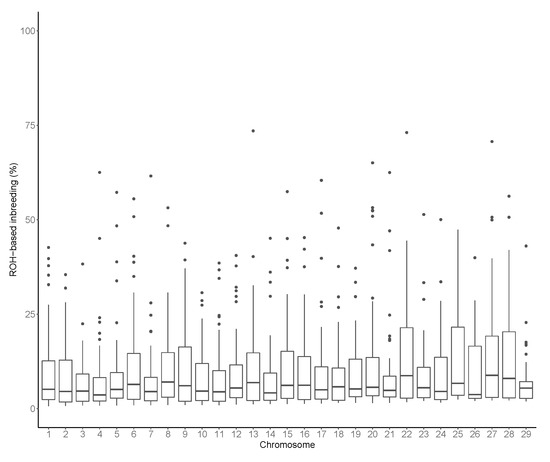
Figure 4.
Runs of homozygosity (ROH) based inbreeding in each considered autosome.
Table 4 shows the correlation between inbreeding coefficients for the group of genotyped animals. The correlations between and or were non-significant (r = −0.25 to 0.31). This and the difference in estimates based on pedigree and genotypes highlights the importance of using genomic information in the assessment of genetic diversity. The use of different measures may lead to different conclusions.
Table 4.
Pearson’s correlations (above diagonal) among genomic (), pedigree () and Runs of Homozygosity () based inbreeding coefficients, significance values 1 are reported below the diagonal.
The correlations among estimates based on different lengths were high (r = 0.69 to 1.00) and significant (p < 0.05), whereas the correlations among estimates and were moderate and non-significant (r = 0.44 to 0.58). Although non-significant, the correlations among and declined as the length increased, which was expected because captures all homozygous segments in the genome, which is not the case for . This would make a better approach to differentiate old and recent inbreeding. Contrary to , inbreeding coefficients estimated using genomic information do not depend on the knowledge of relatives, and therefore, these estimates are not biased by missing or incorrect pedigrees.
Previous studies have reported moderate correlations among and . For example, the correlation between these inbreeding estimates ranged from 0.62 to 0.65 in dairy cattle breeds [49], and it was 0.56 for the Hereford breed [19].
3.2.2. Linkage Disequilibrium and Effective Population Size
The trend over distances between SNP from 100 to 35,000 kb is presented in Figure 5A. The declined from 0.147 to 0.026 when the distance between SNP pairs increased from 102 kb to 32,760 kb. Such observed decay in as the distance between markers increases is a typical trend found in other populations [50,51]. Decay in level was also studied for Romosinuano beef cattle in Colombia by Bejarano et al. [52]. These authors analyzed decay up to 200 and 500 kb and reported larger values than those found for the same distances between SNP in the present study. The observed difference is most likely due to differences in the genetic architecture between the populations. In general, populations under stronger selection have greater levels.
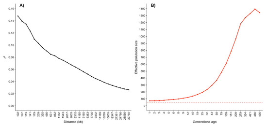
Figure 5.
(A) Linkage disequilibrium estimated through the correlation between pairs of loci () over distances between markers; (B) effective population size trend from 1 to 490 generations ago, the dashed line represents the threshold of 50 proposed as the minimal values to maintain genetic diversity in acceptable levels.
Linkage disequilibrium is a good indicator of associations between alleles of two or more loci. Larger values are usually estimated in homogeneous or closed populations because of loci inheritance from common ancestors. Thus, is greater in selected populations. Since the selection pressure is related to the , can be utilized to estimate [53,54]. The 490 generations ago was 1342 animals, 109 generations ago it was 610, and it was reduced 1 generation ago to 72 (Figure 5B). The latter was a similar value to the of 86.44 14.6 estimated based on the pedigree. Indeed, the estimated using genomic information fell inside the 95% confidence interval (57.82–115.05) for the pedigree-based estimate of . The reduction in moving from the past generations to the recent generations is a common feature of livestock [50,54] and implies a reduction in genetic diversity. It is important to highlight that the estimated 1 generation ago was close to the critical point of 50 animals proposed as the threshold to have acceptable levels of genetic diversity [31]. Therefore, an appropriate mating design is needed to maintain or even increase the genetic diversity within the Mexican Romosinuano beef cattle breed.
3.3. Selection Signatures
A total of 2390 were detected, of which 29% had a length < 1 Mb, 64% had a length from 1 to 2 Mb, and only 7% were longer than 2 Mb. The minimum number of per animal was 25, the maximum was 68, and the mean number was 47.7.
The top 0.01% threshold for was 32.39%, while it was 28.16% for . Only one island was found on chromosome 1 (Figure 6), while three islands were found on chromosomes 1, 8, and 13 (Figure 7).
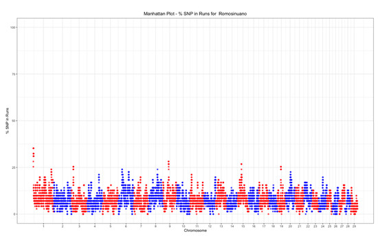
Figure 6.
Manhattan plot of the SNP frequency within runs of homozygosity by autosome in the Mexican Romosinuano beef cattle population.
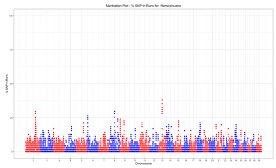
Figure 7.
Manhattan plot of the SNP frequency within runs of heterozygosity by autosome in the Mexican Romosinuano beef cattle population.
Table 5 presents the chromosome position, the start and end of islands on the chromosomes, the number of SNP, and genes found in the and islands. Overall, 22 genes were found on both and islands. The RCAN1 gene was found in the island, and it plays an important role in the proliferation of smooth muscle cells. This gene was previously reported to be associated with the ribeye area in Nellore [55] and Wagyu cattle [56]. The TRNA-CCC gene was reported to be associated with immune-response processes (somatic cell score) and membrane transport in dairy cows and buffalos [57,58]. The KCNE1 and KCNE2 genes were found to be related to growth traits, such as weaning weight in Blanco Orejinegro beef cattle in Colombia, as reported by Londoño-Gil et al. [59].
Table 5.
Description of the runs of homozygosity () and heterozygosity () islands found in the Mexican Romosinuano beef cattle population’s autosomal genome.
Among genes found in islands, the TLEA4 gene is crucial for the function of the mammary gland and has previously been reported in Angus cattle by Devani et al. [60]. Additionally, several genes (CFAP61, RALGAPA2, INSM1, and KIZ) were located in a region associated with feed intake, conformation, weight, reproductive traits, and milk production in cattle, as demonstrated by Pitt et al. [61].
3.4. Inbreeding Depression
Inbreeding depression is a negative consequence of a high rate of inbreeding and can reduce the population’s average performance due to the increased frequency of homozygous alleles that are unfavorable or deleterious [62].
The effects of inbreeding on birth and weaning weights are presented in Table 6. Significant (p < 0.003) effects of inbreeding were found only in the first group of animals (i.e., all the animals with phenotypes). A 1% increase in inbreeding () decreased birth weight by 0.103 kg and weaning weight by 0.685 kg. Similar results were reported by [19] in a research study that used data from the highly inbred line 1 of Hereford cattle in the U.S. In their research, reductions of 0.05 kg in birth weight and 1.2 kg in weaning weight were associated with an increase in of 1%. In the same study, the inbreeding depression was stronger for and than for . In the present study, within the group of animals with genotypes and phenotypes, inbreeding depression was non-significant (p ≥ 0.079) for both pedigree and genomic inbreeding ( or ). These non-significant inbreeding effects are likely attributed to a lack of statistical power due to the small sample size rather than the actual effect of inbreeding on phenotypes.
Table 6.
Estimates of the regression coefficients of pedigree inbreeding , genomic inbreeding based on the genomic relationship matrix and based on runs of homozygosity on birth weight and weaning weight.
Based on a meta-analysis conducted on 57 studies and seven livestock species considering a wide variety of traits under selection, Leroy [63] estimated that inbreeding depression corresponded to an average decrease of 0.137% in the mean of a trait per 1% increase in inbreeding.
Several recent studies investigated the association between production or functional traits and different inbreeding measures (, , and ) [19,36,37]. Martikainen et al. [64] identified that genotypes with high values of had significant unfavorable effects on Finnish Ayrshire cattle fertility traits. Cesarani et al. [39] investigated the effect of the presence/absence of particular on estimated breeding values for milk, fat, and protein in European Simmental bulls and reported that some , shared by at least 20 animals, showed significant adverse effects on all the traits.
A selection strategy to maximize genetic progress and constrain the inbreeding rate should be applied in the Romosinuano Mexican beef cattle population. The optimal genetic contributions method developed by Meuwissen [65] requires the estimated breeding values and relationships among selection candidates. Therefore, it could be easy to implement in this population. The optimal contribution method yields the genetic contributions of selected candidates to the next generations in terms of progeny number per candidate while constraining the average relationship to a given level among selection candidates and, thus, the inbreeding coefficient in the next generation.
4. Conclusions
In the Mexican Romosinuano beef cattle population, the inbreeding coefficient was larger when evaluated based on runs of homozygosity (7.28%) than when estimated based on the pedigree (2.98%) and the genomic relationship matrix (2.98%). Runs of homozygosity of length <4 Mb were more abundant in the autosomal genome. The correlation between and was −0.25, and the correlations among and of different length classes were low and ranged from 0.16 to 0.31. The correlations among and of different length classes were moderate and ranged from 0.44 to 0.58. Genetic bottlenecks were found in the population, and the effective population size presented an important reduction from 610 (109 generations ago) to 72 animals (1 generation ago), which approached the critical value recommended to maintain the genetic diversity at an acceptable level. The reduction in effective population size implies a decline in genetic diversity due to the intensive use of few individuals as parents of the next generations. Selection signatures were detected through highly homozygous and heterozygous regions related to immune response, growth, and reproductive traits. Inbreeding depression analyses showed that a 1% increase in an animal’s pedigree-based inbreeding coefficient resulted in a significant decrease in birth (−0.103 kg) and weaning (−0.685 kg) weights. A strategy, such as optimum genetic contributions to maximize selection response and manage the long-term genetic variability and inbreeding could lead to design more sustainable breeding programs for the Mexican Romosinuano beef cattle breed.
Author Contributions
All authors conceived and validated the study, contributed to methods and to writing the paper; formal analysis, J.H., A.C. and A.G.; data curation, J.H., A.C., A.G. and N.L.; writing—original draft preparation, J.H., A.C., A.G., N.L., P.S. and E.M.; writing—review and editing, J.G.G., R.N. and R.R.; supervision, J.G.G., R.N. and R.R.; All authors have read and agreed to the published version of the manuscript.
Funding
This research received no external funding.
Institutional Review Board Statement
Not applicable.
Informed Consent Statement
Not applicable.
Data Availability Statement
The dataset is not publicly available since it belongs to “Asociación Mexicana de Criadores de Ganado Romosinuano y Lechero Tropical” and is treated as confidential information.
Acknowledgments
The authors are grateful to Yvette Steyn for his useful input and greatly appreciate the availability of data from “Asociación Mexicana de Criadores de Ganado Romosinuano y Lechero Tropical”. Jorge Hidalgo acknowledges the support during his PhD studies by the National Council for Science and Technology (CONACYT), Mexico.
Conflicts of Interest
The authors declare no conflict of interest.
References
- De Alba, J. El libro de los Bovinos Criollos de América; Biblioteca Básica Agricultura (BBA): México City, Mexico, 2011. [Google Scholar]
- Ramírez Valverde, R.; Martínez Rocha, R.E.; Núñez Domínguez, R.; García Muñiz, J.G. Genetic parameters and trends of growth traits for Romosinuano cattle in Mexico. Nova Sci. 2018, 10, 16. [Google Scholar] [CrossRef]
- Núñez-Domínguez, R.E.; Martínez-Rocha, R.; Hidalgo-Moreno, J.; Ramírez-Valverde, R.; García-Muñiz, J.G. Evaluation of the Romosinuano cattle population structure in Mexico using pedigree analysis. Rev. Colomb. Cienc. Pecu. 2020, 33. [Google Scholar] [CrossRef]
- Gutiérrez, J.P.; Altarriba, J.; Díaz, C.; Quintanilla, R.; Cañón, J.; Piedrafita, J. Pedigree analysis of eight Spanish beef cattle breeds. Genet. Sel. Evol. 2003, 35, 43. [Google Scholar] [CrossRef] [PubMed]
- VanRaden, P.M. Accounting for Inbreeding and Crossbreeding in Genetic Evaluation of Large Populations. J. Dairy Sci. 1992, 75, 3136–3144. [Google Scholar] [CrossRef]
- Purcell, S.; Neale, B.; Todd-Brown, K.; Thomas, L.; Ferreira, M.A.R.; Bender, D.; Maller, J.; Sklar, P.; de Bakker, P.I.W.; Daly, M.J.; et al. PLINK: A Tool Set for Whole-Genome Association and Population-Based Linkage Analyses. Am. J. Hum. Genet. 2007, 81, 559–575. [Google Scholar] [CrossRef]
- Gutiérrez, J.P.; Goyache, F. A note on ENDOG: A computer program for analysing pedigree information. J. Anim. Breed. Genet. 2005, 122, 172–176. [Google Scholar] [CrossRef]
- Malécot, G. Mathématiques de l’hérédité. 1948. Available online: https://www.persee.fr/doc/linly_0366-1326_1948_num_17_10_8510_t1_0203_0000_2 (accessed on 9 November 2020).
- Meuwissen, T.H.E.; Luo, Z. Computing inbreeding coefficients in large populations. Genet. Sel. Evol. 1992, 24, 305–313. [Google Scholar] [CrossRef]
- Boichard, D.; Maignel, L.; Verrier, E. The value of using probabilities of gene origin to measure genetic variability in a population. Genet. Sel. Evol. 1997, 29, 1–19. [Google Scholar] [CrossRef]
- Maignel, L.; Boichard, D.; Verrier, E. Genetic variability of French dairy breeds estimated from pedigree information. Interbull Bull. 1996, 49. [Google Scholar]
- MacCluer, J.W.; Boyce, A.J.; Dyke, B.; Weitkamp, L.R.; Pfenning, D.W.; Parsons, C.J. Inbreeding and pedigree structure in Standardbred horses. J. Hered. 1983, 74, 394–399. [Google Scholar] [CrossRef]
- Gutiérrez, J.P.; Cervantes, I.; Molina, A.; Valera, M.; Goyache, F. Individual increase in inbreeding allows estimating effective sizes from pedigrees. Genet. Sel. Evol. 2008, 40, 1–20. [Google Scholar] [CrossRef] [PubMed]
- Gutiérrez, J.; Cervantes, I.; Goyache, F. Improving the estimation of realized effective population sizes in farm animals. J. Anim. Breed. Genet. 2009, 126, 327–332. [Google Scholar] [CrossRef] [PubMed]
- Lacy, R.C. Analysis of founder representation in pedigrees: Founder equivalents and founder genome equivalents. Zoo Biol. 1989, 8, 111–123. [Google Scholar] [CrossRef]
- VanRaden, P.M. Efficient methods to compute genomic predictions. J. Dairy Sci. 2008, 91, 4414–4423. [Google Scholar] [CrossRef] [PubMed]
- Misztal, I.; Tsuruta, S.; Lourenco, D.A.L.; Masuda, Y.; Aguilar, I.; Legarra, A.; Vitezica, Z. Manual for BLUPF90 Family of Programs. 2014. Available online: http://nce.ads.uga.edu/wiki/lib/exe/fetch.php?media=blupf90_all2.pdf (accessed on 4 May 2020).
- Zhang, Q.; Calus, M.P.L.; Guldbrandtsen, B.; Lund, M.S.; Sahana, G. Estimation of inbreeding using pedigree, 50k SNP chip genotypes and full sequence data in three cattle breeds. BMC Genet. 2015, 16, 88. [Google Scholar] [CrossRef] [PubMed]
- Sumreddee, P.; Toghiani, S.; Hay, E.H.; Roberts, A.; Agrrey, S.E.; Rekaya, R. Inbreeding depression in line 1 Hereford cattle population using pedigree and genomic information1. J. Anim. Sci. 2018, 97, 1–18. [Google Scholar] [CrossRef] [PubMed]
- Biscarini, F.; Cozzi, P.; Gaspa, G.; Marras, G. DetectRUNS: Detect Runs of Homozygosity and Runs of Heterozygosity in Diploid Genomes, 0.9.5. 2018. Available online: https://github.com/bioinformatics-ptp/detectRUNS/tree/master/detectRUNS (accessed on 4 May 2020).
- Kirin, M.; McQuillan, R.; Franklin, C.S.; Campbell, H.; McKeigue, P.M.; Wilson, J.F. Genomic Runs of Homozygosity Record Population History and Consanguinity. PLoS ONE 2010, 5, e13996. [Google Scholar] [CrossRef]
- Cesarani, A.; Sorbolini, S.; Criscione, A.; Bordonaro, S.; Pulina, G.; Battacone, G.; Marletta, D.; Gaspa, G.; Macciotta, N.P.P. Genome-wide variability and selection signatures in Italian island cattle breeds. Anim. Genet. 2018, 49, 371–383. [Google Scholar] [CrossRef]
- Barbato, M.; Orozco-terWengel, P.; Tapio, M.; Bruford, M.W. SNeP: A tool to estimate trends in recent effective population size trajectories using genome-wide SNP data. Front. Genet. 2015, 6, 109. [Google Scholar] [CrossRef]
- Corbin, L.J.; Liu, A.; Bishop, S.; Woolliams, J. Estimation of historical effective population size using linkage disequilibria with marker data. J. Anim. Breed. Genet. 2012, 129, 257–270. [Google Scholar] [CrossRef]
- Hayes, B.J.; Visscher, P.M.; McPartlan, H.C.; Goddard, M.E. Novel multilocus measure of linkage disequilibrium to estimate past effective population size. Genome Res 2003, 13, 635–643. [Google Scholar] [CrossRef] [PubMed]
- Sved, J.; Feldman, M. Correlation and probability methods for one and two loci. Theor. Popul. Biol. 1973, 4, 129–132. [Google Scholar] [CrossRef]
- Tenesa, A.; Navarro, P.; Hayes, B.J.; Duffy, D.L.; Clarke, G.M.; Goddard, M.E.; Visscher, P.M. Recent human effective population size estimated from linkage disequilibrium. Genome Res 2007, 17, 520–526. [Google Scholar] [CrossRef]
- Biscarini, F.; Mastrangelo, S.; Catillo, G.; Senczuk, G.; Ciampolini, R. Insights into Genetic Diversity, Runs of Homozygosity and Heterozygosity-Rich Regions in Maremmana Semi-Feral Cattle Using Pedigree and Genomic Data. Animals 2020, 10, 2285. [Google Scholar] [CrossRef] [PubMed]
- R Core Team. R: A Language and Environment for Statistical Computing; R Foundation for Statistical Computing: Vienna, Austria, 2020. [Google Scholar]
- Barczak, E.; Wolc, A.; Wójtowski, J.; Ślósarz, P.; Szwaczkowski, T. Inbreeding and inbreeding depression on body weight in sheep. J. Anim. Feed Sci. 2009, 18, 42–50. [Google Scholar] [CrossRef]
- FAO. Secondary Guidelines for Development of National Farm Animal Genetic Resources Management Plans: Management of Small Populations at Risk; FAO: Rome, Italy, 1998. [Google Scholar]
- Ramírez-Valverde, R.; Delgadillo-Zapata, A.R.; Domínguez-Viveros, J.; Hidalgo-Moreno, H.A.; Núñez-Domínguez, R.; Rodriguez-Almedida, F.A.; Reyes-Quiroz, C.; García-Muñiz, J.G. Pedigree analysis for determination of genetic diversity in Mexican beef cattle populations. Rev. Mex. Cienc. Pecu. 2018, 9, 614–635. [Google Scholar] [CrossRef]
- Maltecca, C.; Tiezzi, F.; Cole, J.B.; Baes, C. Symposium review: Exploiting homozygosity in the era of genomics-Selection, inbreeding, and mating programs. J. Dairy Sci. 2020, 103, 5302–5313. [Google Scholar] [CrossRef]
- Broman, K.W.; Weber, J.L. Long homozygous chromosomal segments in reference families from the centre d’Etude du polymorphisme humain. AJHG 1999, 65, 1493–1500. [Google Scholar] [CrossRef]
- Purfield, D.C.; Berry, D.P.; McParland, S.; Bradley, D.G. Runs of homozygosity and population history in cattle. BMC Genet. 2012, 13, 70. [Google Scholar] [CrossRef]
- Doekes, H.P.; Veerkamp, R.F.; Bijma, P.; de Jong, G.; Hiemstra, S.J.; Windig, J.J. Inbreeding depression due to recent and ancient inbreeding in Dutch Holstein–Friesian dairy cattle. Genet. Sel. Evol. 2019, 51, 54. [Google Scholar] [CrossRef]
- Makanjuola, B.O.; Maltecca, C.; Miglior, F.; Schenkel, F.S.; Baes, C.F. Effect of recent and ancient inbreeding on production and fertility traits in Canadian Holsteins. BMC Genom. 2020, 21, 605. [Google Scholar] [CrossRef] [PubMed]
- Sumreddee, P.; Toghiani, S.; Hay, E.H.; Roberts, A.; Aggrey, S.E.; Rekaya, R. Runs of homozygosity and analysis of inbreeding depression. J. Anim. Sci. 2020, 98, skaa361. [Google Scholar] [CrossRef] [PubMed]
- Cesarani, A.; Gaspa, G.; Pauciullo, A.; Degano, L.; Vicario, D.; Macciotta, N.P.P. Genome-wide analysis of homozygosity regions in european simmental bulls. J. Anim. Breed. Genet. 2020. [Google Scholar] [CrossRef] [PubMed]
- Marras, G.; Gaspa, G.; Sorbolini, S.; Dimauro, C.; Ajmone-Marsan, P.; Valentini, A.; Williams, J.L.; Macciotta, N.P.P. Analysis of runs of homozygosity and their relationship with inbreeding in five cattle breeds farmed in Italy. Anim. Genet. 2015, 46, 110–121. [Google Scholar] [CrossRef]
- Curik, I.; Ferenčaković, M.; Sölkner, J. Inbreeding and runs of homozygosity: A possible solution to an old problem. Livest. Sci. 2014, 166, 26–34. [Google Scholar] [CrossRef]
- Gibson, J.; Morton, N.E.; Collins, A. Extended tracts of homozygosity in outbred human populations. Hum. Mol. Genet. 2006, 15, 789–795. [Google Scholar] [CrossRef]
- Bosse, M.; Megens, H.-J.; Madsen, O.; Paudel, Y.; Frantz, L.A.F.; Schook, L.B.; Crooijmans, R.P.M.A.; Groenen, M.A.M. Regions of Homozygosity in the Porcine Genome: Consequence of Demography and the Recombination Landscape. PLoS Genet. 2012, 8, e1003100. [Google Scholar] [CrossRef]
- Fisher, R.A. A fuller theory of “Junctions” in inbreeding. Heredity 1954, 8, 187–197. [Google Scholar] [CrossRef]
- Ferencakovic, M.; Hamzić, E.; Gredler, B.; Solberg, T.R.; Klemetsdal, G.; Curik, I.; Sölkner, J. Estimates of autozygosity derived from runs of homozygosity: Empirical evidence from selected cattle populations. J. Anim. Breed. Genet. 2013, 130, 286–293. [Google Scholar] [CrossRef]
- Szmatoła, T.; Gurgul, A.; Ropka-Molik, K.; Jasielczuk, I.; Ząbek, T.; Bugno-Poniewierska, M. Characteristics of runs of homozygosity in selected cattle breeds maintained in Poland. Livest. Sci. 2016, 188, 72–80. [Google Scholar] [CrossRef]
- Ferencakovic, M.; Hamzi, E.; Gredler, B.; Curik, I.; Sölkner, J. Runs of Homozygosity Reveal Genome- Wide Autozygosity in the Austrian Fleckvieh Cattle. Agr. Cons. Sci. 2011, 76, 325–328. Available online: http://www.agr.unizg.hr/smotra/pdf_76/acs76_63.pdf (accessed on 4 July 2020).
- Meyermans, R.; Gorssen, W.; Buys, N.; Janssens, S. How to study runs of homozygosity using PLINK? A guide for analyzing medium density SNP data in livestock and pet species. BMC Genom. 2020, 21, 94. [Google Scholar] [CrossRef] [PubMed]
- Pryce, J.E.; Haile-Mariam, M.; Goddard, M.E.; Hayes, B.J. Identification of genomic regions associated with inbreeding depression in Holstein and Jersey dairy cattle. Genet. Sel. Evol. 2014, 46, 71. [Google Scholar] [CrossRef] [PubMed]
- Sargolzaei, M.; Schenkel, F.S.; Jansen, G.B.; Schaeffer, L.R. Extent of Linkage Disequilibrium in Holstein Cattle in North America. J. Dairy Sci. 2008, 91, 2106–2117. [Google Scholar] [CrossRef] [PubMed]
- Xu, L.; Zhu, B.; Wang, Z.; Xu, L.; Liu, Y.; Chen, Y.; Zhang, L.; Gao, X.; Gao, H.; Zhang, S.; et al. Evaluation of Linkage Disequilibrium, Effective Population Size and Haplotype Block Structure in Chinese Cattle. Animals 2019, 9, 83. [Google Scholar] [CrossRef]
- Bejarano, D.; Martínez, R.; Manrique, C.; Parra, L.M.; Rocha, J.F.; Gómez, Y.; Abuabara, Y.; Gallego, J. Linkage disequilibrium levels and allele frequency distribution in Blanco Orejinegro and Romosinuano Creole cattle using medium density SNP chip data. Genet. Mol. Biol. 2018, 41, 426–433. [Google Scholar] [CrossRef]
- Bohmanova, J.; Sargolzaei, M.; Schenkel, F.S. Characteristics of linkage disequilibrium in North American Holsteins. BMC Genom. 2010, 11, 421. [Google Scholar] [CrossRef]
- Flury, C.; Tapio, M.; Sonstegard, T.; Drögemüller, C.; Leeb, T.; Simianer, H.; Hanotte, O.; Rieder, S. Effective population size of an indigenous Swiss cattle breed estimated from linkage disequilibrium. J. Anim. Breed. Genet. 2010, 127, 339–347. [Google Scholar] [CrossRef]
- Silva, D.B.; Fonseca, L.F.; Pinheiro, D.G.; Magalhães, A.F.; Muniz, M.M.; Ferro, J.A.; Baldi, F.; Chardulo, L.A.; Schnabel, R.D.; Taylor, J.F. Spliced genes in muscle from Nelore Cattle and their association with carcass and meat quality. Sci. Rep. 2020, 10, 1–13. [Google Scholar] [CrossRef]
- Zhang, L.; Michal, J.J.; O’Fallon, J.V.; Pan, Z.; Gaskins, C.T.; Reeves, J.J.; Busboom, J.R.; Zhou, X.; Ding, B.; Dodson, M.V. Quantitative genomics of 30 complex phenotypes in Wagyu × Angus F1 progeny. Int. J. Biol. Sci. 2012, 8, 838. [Google Scholar] [CrossRef][Green Version]
- Grajales, S.M.B.; Zuluaga, J.J.E.; Herrera, A.L.; Osorio, N.R.; Vergara, D.M.B. RNA-seq differential gene expression analysis in mammary tissue from lactating dairy cows supplemented with sunflower oil. Anim. Prod. Sci. 2020, 60, 758–771. [Google Scholar] [CrossRef]
- De Camargo, G.; Aspilcueta-Borquis, R.R.; Fortes, M.; Porto-Neto, R.; Cardoso, D.F.; Santos, D.; Lehnert, S.; Reverter, A.; Moore, S.; Tonhati, H. Prospecting major genes in dairy buffaloes. BMC Genom. 2015, 16, 872. [Google Scholar] [CrossRef] [PubMed]
- Londoño-Gil, M.; Rincón Flórez, J.C.; Lopez-Herrera, A.; Gonzalez-Herrera, L.G. Genome-Wide Association Study for Growth Traits in Blanco Orejinero (Bon) Cattle from Colombia. Livest. Sci. 2021, 243, 104366. [Google Scholar] [CrossRef]
- Devani, K.; Plastow, G.; Orsel, K.; Valente, T.S. Genome-wide association study for mammary structure in Canadian Angus cows. PLoS ONE 2020, 15, e0237818. [Google Scholar] [CrossRef]
- Pitt, D.; Bruford, M.W.; Barbato, M.; Orozco-terWengel, P.; Martínez, R.; Sevane, N. Demography and rapid local adaptation shape Creole cattle genome diversity in the tropics. Evol. Appl. 2019, 12, 105–122. [Google Scholar] [CrossRef]
- Falconer, D.S.; Mackay, T.F.C. Introduction to Quantitative Genetics, 4th ed.; Longman: Essex, UK, 1996. [Google Scholar]
- Leroy, G. Inbreeding depression in livestock species: Review and meta-analysis. Anim. Genet. 2014, 45, 618–628. [Google Scholar] [CrossRef]
- Martikainen, K.; Sironen, A.; Uimari, P. Estimation of intrachromosomal inbreeding depression on female fertility using runs of homozygosity in Finnish Ayrshire cattle. J. Dairy Sci. 2018, 101, 11097–11107. [Google Scholar] [CrossRef]
- Meuwissen, T.H.E. Maximizing the response of selection with a predefined rate of inbreeding. J. Anim. Sci. 1997, 75, 934–940. [Google Scholar] [CrossRef]
Publisher’s Note: MDPI stays neutral with regard to jurisdictional claims in published maps and institutional affiliations. |
© 2021 by the authors. Licensee MDPI, Basel, Switzerland. This article is an open access article distributed under the terms and conditions of the Creative Commons Attribution (CC BY) license (http://creativecommons.org/licenses/by/4.0/).