Abstract
Magnetorheological (MR) damper performance is evaluated only by single-field analysis in the design process, which can easily lead to larger design errors. Based on this, a simulation method of MR damper considering multiphysics coupling was proposed. According to a certain automobile shock absorber requirement, an MR damper suitable for automobile suspension was designed. The mechanical model, electromagnetic field model, flow field model, and structural stress field model of the MR damper were deduced and established. To investigate the damping performance of the MR damper more accurately, the multiphysics coupling simulation model was established by COMSOL software, and coupling analysis of the electromagnetic field, flow field, and structural stress field was also carried out. The static magnetic field characteristics, dynamic flow field characteristics, stress distribution, and dynamic performance of the proposed MR damper under the action of multiphysics coupling were obtained. The simulation results show that the damping force is 1134.6 N, and the damping adjustable coefficient is 9.1 at an applied current of 1.4 A. A test system was established to analyze the dynamic performance of the MR damper, and the simulation results were compared with the experimental results. The results show that the simulated and experimental results have the same change rule. Moreover, the damping force increases with the applied current, and different external excitations have little effect on the damping force. The damper can output appropriate damping force and has a wide adjustable damping range. The experimental results illustrate that the damping force is 1200.0 N, and the damping adjustable coefficient is 10.1 when the current is 1.4 A. The error between simulation and experiment of the damping force and damping adjustable coefficient is only 5.5% and 9.9%, respectively.
1. Introduction
Hydraulic dampers are commonly used in conventional vehicle suspensions system. However, it is difficult to have good driving comfort and handling stability under different driving conditions due to the unchangeable spring stiffness and dynamic range.
As a representative magnetorheological (MR) actuator, the MR damper is a new generation of intelligent shock absorbers. Compared with conventional hydraulic dampers, MR dampers have the advantages of simple structure, fast response, large output damping force and continuous controllability [1,2]. It is an excellent semi-active damping device and can be widely used in transportation and other fields, such as automobile suspension systems. And it is beneficial to improve the comfort and running quality of the vehicle [3,4,5,6,7,8,9].
As a critical device in vibration damping systems, the engineering design of an MR damper directly impacts its performance index, and a reasonable simulation can get the best design scheme in the shortest time with the least manpower and material resources [10,11,12]. Therefore, domestic and foreign scholars have performed a lot of research on the simulation of MR dampers, and magnetic field simulation is the most common technical method [13,14,15]. Yang et al. [16] designed a three-coil MR damper and established a finite element model based on the theoretical analysis of the magnetic circuit. The magnetic field intensity in the damping gap was calculated by simulation under different currents and coil turns. Mangal et al. [17] designed an MR damper and simulated it with ANSYS software. The validity of the finite element simulation analysis was verified through experiments. The maximum damping force was 500 N, and the damping force error between the experiment and the simulation was about 10%. Olivier et al. [18] proposed a hybrid MR damper in which the magnetic field is jointly provided by both an electromagnet and a permanent magnet. To analyze its magnetic field characteristics, the internal magnetic field distribution of the damper was obtained by simulation when only a permanent magnet acted on it and when electromagnet and permanent magnet acted on it together. Ganesha et al. [19] designed a single-coil twin-tube MR damper. To research the influence of the built-in magnetic shielding layer on the magnetic field, the magnetic field enhancement technologies of single cylinder shielding and sandwich cylinder shielding were introduced into the damper, and the magnetic flux density of the damper under different shielding structures was obtained through simulation. Golinelli et al. [20] presented a MR damper of a new structure with controllable internal pressure. The magnetic field of the damper was simulated by finite element software. Combined with the experimental results, it was shown that the minimum damping force error between the experiment and the simulation was about 8.2%, and the maximum error was about 15%. Hu et al. [21] developed an MR damper with serial-type flow channels. The damper’s piston passed through three damping channels in series, which greatly extended the damping length of the fluid flow. The magnetic field simulation results show that the structure of the damper makes full use of the magnetic flux lines and can improve the damping force.
In the above research, only a single physical field was considered in the design stage for magnetic field analysis. However, due to the particularity of the MR fluid, the MR damper has become a complex system that integrates electromagnetics, fluid mechanics, and solid mechanics. Therefore, its performance is affected by multiphysics [22,23,24,25]. In the design, only a single field analysis has been used to evaluate the performance of the damper, which quickly leads to significant design errors. Therefore, to predict MR damper’s performance more accurately in the design stage, it is of great engineering significance and practical value to carry out simulation research on it under the coupling effect of multiphysics.
This paper designed an MR damper according to the needs of a light-duty automobile shock absorber, which requires the damping force greater than 1000 N. To more accurately discuss the overall performance of the proposed damper, a multiphysics coupling simulation method was proposed, and COMSOL software was used to solve and analyze the damper under the interaction of electromagnetic field, flow field and structural stress field. The static magnetic field characteristics, dynamic flow field characteristics, stress distribution and dynamic performance curves of the damper under multiphysics coupling are explored by simulation. The feasibility of the proposed damper and the accuracy of the multiphysics coupling simulation model in this paper were verified through experiments.
2. Structure and Principle of Proposed MR Damper
2.1. Structural Design
An MR damper, as shown in Figure 1, was designed to meet the requirements of an automobile suspension shock absorber. The damper is mainly composed of a lifting lug, piston rod, screw, end cover, cylinder block, excitation coil, piston head, and end shield. It is a double-rod damper functioning under shear and valve mode. The left and right piston rods are connected as a whole through the thread, and thus the piston head is fixed between the two piston rods; The excitation coil is evenly wound in the bobbin on the piston head, and it is led out of the damper through the lead hole on the piston head and piston rod. The piston head divides the inside of the damper into left and right chambers. And the chamber is filled with MR fluid. The annular gap between the piston head and the cylinder forms a damping gap connecting the two chambers, and the thickness of the damping gap is 1 mm. To facilitate liquid injection and installation, two liquid injection holes are evenly opened on the left end cover, and an end shield is provided on the right end cover.

Figure 1.
Schematic diagram of MR damper. (1) Left lifting lug, (2) left piston rod, (3) injection hole screw, (4) left end cover, (5) cylinder, (6) excitation coil, (7) piston head, (8) right piston rod, (9) right end cover, (10) end cover screw, (11) end shield, (12) right lifting lug.
2.2. Working Principle
Different from conventional dampers, the output damping force of MR dampers is controlled by the excitation current. The structure of the proposed damper was properly simplified, and relevant design parameters were extracted. The working principle is shown in Figure 2.
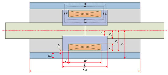
Figure 2.
Working principle of the developed MR damper.
When the damper is stimulated by vibration, the reciprocating motion of the piston head will cause volume change of the left and right chambers, thus forcing the MR fluid to flow through the damping channel. The excitation coil is evenly wound in the piston head. When the excitation coil is energized, a magnetic field will be generated around the coil due to the galvanomagnetic effect. The magnetic flux lines pass through the piston head and the cylinder successively and form a closed loop through the damping channel vertically. MR fluids will produce the rheological effect in the damping gap with a magnetic field [26,27], and controlling the current of the excitation coil can change the magnetic field intensity inside the damping gap. This causes the viscosity and shear yield stress of the MR fluid flowing through the channel to change, leading to the pressure difference between the two chambers change, thereby achieving a control effect on the output damping force.
3. Mathematical Models of Proposed MR Damper
3.1. Mechanical Model
According to the Bingham pseudo-static model, the output damping force is the sum of viscosity-induced and magnetically induced damping forces when the MR damper is energized:
where Fη is viscosity-induced damping force, and Fτ is magnet-induced damping force.
When the damper under shear valve mode is excited, the MR fluid in the chamber can be considered to have both shear flow and differential pressure flow. The output damping force is divided into the damping force generated in the shear and valve modes [28,29].
where Fs is the damping force in the shear mode, and Fp is the damping force in valve mode.
The viscosity-induced damping force in shear mode is:
The viscosity-induced damping force in valve mode is:
For the MR damper under shear valve mode, the viscosity-induced damping force generated by its velocity is the sum of Equations (3) and (4):
The magnetically-induced damping force in shear mode is:
The magnetically induced damping force in valve mode is:
In a similar way, the magnetically induced damping force generated by its magnetic field is the sum of Equations (6) and (7):
By substituting Equations (5) and (8) into Equation (1), the output damping force of the proposed MR damper is:
where η is the viscosity of the MR fluid without magnetic field; Ap is the effective area of piston; v is the velocity of the piston relative to the cylinder; c is the correction factor (its value is 3), and τy is the yield stress of the MR fluid on the flank of the damping gap.
In Equation (9), the first term is related to velocity and represents the sum of viscosity-induced damping forces in the damper. The second term is associated with the magnetic field and represents the sum of the magnetically induced damping forces in the damper. Since the viscosity-induced damping force is mainly caused by the viscosity of the MR fluid, its magnitude is mainly related to the selected MR fluid type and the damper structure. When the MR damper works normally, the magnetically induced damping force is generally much larger than the viscosity-induced damping force, and the damping force is almost entirely provided by the magnetically induced damping force. The larger the difference between them, the more adjustable the performance of the damper will be. When the damper is powered off, the appropriate viscosity-induced damping force will enhance the safety of the MR damper. To evaluate the damping adjustable performance of an MR damper, the ratio of magnetic and viscosity-induced damping forces is often used as its dynamic range, β, namely:
3.2. Electromagnetic Field Model
The internal static magnetic field analysis of the MR damper can be solved by Maxwell’s equations. According to the current law of the electromagnetic field, vector H of the magnetic field intensity for the static magnetic field satisfies the Ampere circuital theorem:
where is the Hamiltonian operator and J is the current density.
Here, the current density, J, can be expressed as:
where σ is the conductivity, v is the conductor velocity, B is the magnetic flux density, and Je is the external current density.
The relationship between magnetic flux density B and magnetic potential A is as follows:
The relationship between magnetic flux density B and magnetic field intensity H is as follows:
where μ0 is the vacuum permeability and M is the magnetization.
Substituting Equations (12) to (14) into Equation (11), the expression of the Ampere circuital theorem is:
When analyzing the static magnetic field of the MR damper, it is necessary to consider the different electromagnetic properties of the material, and define the solution domain of the two Ampere circuital theorems.
For areas with non-magnetic materials or materials with fixed permeability, such as stainless steel and excitation coils, the Ampere circuital theorem can be denoted as:
where μr is the relative permeability of the material.
For the region of nonlinear soft magnetic materials such as MR fluid and No.10 low carbon steel, the Ampere circuital theorem can be expressed as:
The B–H curve of nonlinear soft magnetic materials can be regarded as:
Regardless of the weak eddy current generated by the excitation coil reciprocating with the piston, i.e., σv × B = 0, then the current excitation of the electromagnetic field is only provided by the excitation coil. From Equation (12), the current density, J, can be expressed as:
where N is the number of excitation coil turns; I is the excitation current; Sc is the cross-sectional area of the excitation coil; and en is the unit vector of the direction of motion of the positive charge.
In combination with Equations (13) and (16) to (19), the electromagnetic field distribution inside the MR damper can be described as:
3.3. Flow Field Model
When analyzing the internal flow field of the MR damper, the MR fluid is regarded as an incompressible single-phase fluid that is not affected by temperature. Then the flow of the MR fluid in the damper can be described by the Navier–Stokes equation:
where ρ1 is the fluid density, u1 is the flow velocity, I is the identity matrix, p is pressure, μ is dynamic viscosity, and Fv is the volume force.
The flow pattern of MR fluid in the damping gap can be determined by Reynolds number Re:
Since the damping gap thickness, h, is only 1 mm; the Re value estimated by substituting data is far less than 2320, so the MR fluid can be judged to be in a laminar flow state.
For steady-state laminar flow analysis, Equation (21) can be further simplified as:
When the MR fluid is under the action of a magnetic field, the shear stress, τ, it generates is related to the yield stress, τy, and the shear rate, . According to the Bingham–Papanastasiou model of non-Newtonian fluids, the shear stress of the MR fluid after yielding is expressed as:
where μρ is the plastic viscosity, and both the yield stress, τy, and the model parameter, mρ, can be defined by a polynomial of the magnetic flux density B.
Dividing both sides of Equation (24) by , the dynamic viscosity can be obtained as:
The volume force, Fv, of the MR fluid in a magnetic environment is the magnetic penetration force generated under the action of a magnetic field, namely:
In combination with Equations (23), (25), and (26), the internal flow field distribution of the MR damper can be described as:
3.4. Structural Stress Field Model
Navier–Stokes coupling equations can be used to analyze and solve for the fluid domain with the magnetic field. For the solid domain, its transient state calculation of solid local Equation is:
where ρ2 is the material density, ds is the structural displacement, and σk is the quadratic Cauchy stress tensor.
The arbitrary Lagrangian–Euler (ALE) method was used to couple the fluid domain and the solid domain. The resultant force, fs, of the fluid acting on the fluid-solid coupling boundary is:
where n is the normal vector of the fluid-solid coupling boundary.
The force, Fs, on the solid domain can be obtained by the Cauchy stress tensor, σk:
Coupling the force on the boundary between the solid and fluid domains in the material coordinate system and the space coordinate system, the following can be obtained:
where z is the scale factor of mesh element, Z is the frame of material and fluid.
The rate of change of the structural displacement, dS, is called the structural velocity, u2, namely:
Assuming that there is no slip at the fluid–solid coupling boundary, The velocity, u1, of the MR fluid is equal to the structural velocity, u2, then:
In connection with Equations (28) to (33), the stress field distribution of the internal structure of the MR damper can be described as:
4. Multiphysics Coupling Simulation of the Proposed MR Damper
For the MR damper, the magnetic flux density distribution of the electromagnetic field affects the MR fluid. The viscosity of the MR fluid under different magnetic field intensities will also be different, and the external shock excitation will also affect the state of the flow field. Therefore, the MR damper, as a complex research object, has interactions between different physical fields.
Figure 3 shows the coupling relationship between the physical fields of the MR damper. For the magneto–fluid coupling process, the effect of the electromagnetic field on the internal flow field of the damper is more prominent. In contrast, the effect of the flow field on the electromagnetic field is relatively small so that it can be regarded as a unidirectional coupling effect. In the whole process of magneto–fluid–solid coupling analysis, the movement of the damper causes the flow state of the MR fluid to change, and the load of the fluid reacts on the damper to produce stress and strain in the structure.

Figure 3.
The coupling relationship of the physical fields of the MR damper.
4.1. Simulation Model
The performance of an MR damper is related to its internal electromagnetic field, flow field distribution and damper structure. To explore the distribution and change laws of the internal electromagnetic field and flow field of the proposed damper when it is energized, and thus obtain the dynamic performance of the damper under the action of multiphysics coupling, a simulation model, as shown in Figure 4, was established by COMSOL software (Version 5.4) according to the structural parameters in Table 1. Considering that the proposed damper is a regular axisymmetric body about the central axis, to simplify the calculation, the model dimension is set to two-dimensional axisymmetric [30], and the 1/2 section of the damper is taken as the simulation object without affecting the accuracy.
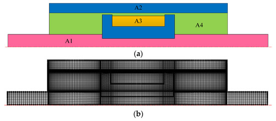
Figure 4.
Simulation model of the MR damper. (a) Entity model, (b) finite element model.

Table 1.
Key structural parameters of MR damper.
Figure 4a shows the simulation solid model, which can be divided into four parts according to the material properties in each area. Among them, A1 is the piston rod, which is a non-magnetic material. 40CrNi2Mo stainless steel with weak magnetic conductivity was adopted, and its relative permeability was defined as 1. A2 is the cylinder and piston head. It is a magnetic material, and it is made of No.10 low carbon steel with good magnetic conductivity and structural strength. A3 is the excitation coil part, which is wound with enamelled copper wire evenly with multiple turns. It is regarded as a uniform material with a relative permeability equal to 1. A4 is MRF-J25T type MR fluid (from Chongqing Materials Research Institute in China), its electromagnetic properties are customized in the form of a B–H curve, and its material properties were shown in Table 2. Figure 4b shows the finite element model after meshing, and the solid model is divided by using quadrilateral mapping mesh. To improve the calculation speed without affecting the simulation accuracy, the processing meshes are required to be dense, and the critical areas such as the damping gap and fluid-solid contact boundary need to be precisely divided.

Table 2.
Properties of MRF-J25T.
As a kind of non-Newtonian fluid whose viscosity varies with magnetic flux density and shear rate, the rheological properties of the MR fluid are the critical medium for coupling the magnetic field and flow field in the damper. According to the test data provided by the material supplier and based on the Bingham–Papanastasiou model of non-Newtonian fluids, the optimal theory and ordinary least squares were adopted to identify the original data, and the characteristic surface of MRF-J25T was obtained, as shown in Figure 5. Its mathematical expression is:
where: .
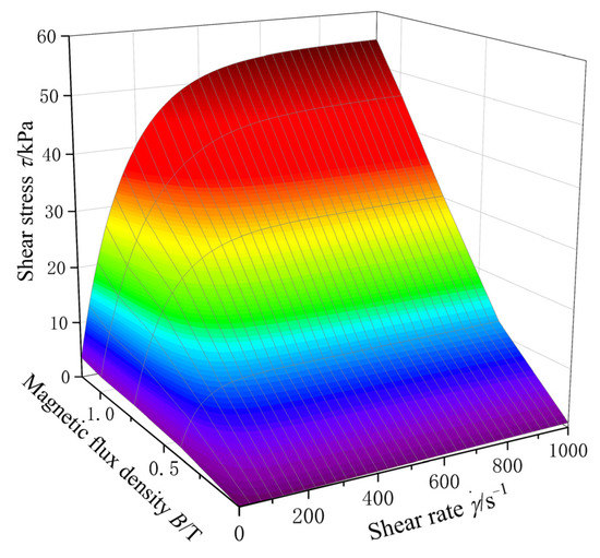
Figure 5.
Characteristic surface of the used MR fluid with the type of MRF-J25T.
In order to dynamically simulate the process of the vibration of the damper, the arbitrary Lagrangian–Euler (ALE) method was used to process the dynamic mesh of the simulation model, and the motion equation specifies the displacement state of the piston. The simulation model can be divided into four deformation domains according to the motion form of the piston, as shown in Figure 6. Three simulation boundaries were defined; boundaries 1 and 2 are the fluid–solid coupling boundary and boundary 3 is the electromagnetic field boundary. The moving wall condition consistent with the piston motion equation was applied to boundary 1. The non-sliding fixed wall condition was applied to boundary 2, and the magnetic field parallel condition was applied to boundary 3.

Figure 6.
Deformation domain and boundary conditions of dynamic mesh.
4.2. Simulation Analysis of Electromagnetic Field
In the magnetic field simulation, the electromagnetic field simulation of the damper is treated as a two-dimensional static magnetic field problem without considering the transient process of excitation current and the weak eddy current generated when the piston moves. Only the state of its internal stable magnetic field was analyzed. The current density was applied to the excitation coil area according to Equation (19). The distribution of the electromagnetic field inside the proposed damper when the given current was 1 A is shown in Figure 7. According to the distribution of the magnetic field, the damping gap can be divided into three sections, S1, S2, and S3. The sections S1 and S3 are where the magnetic flux lines are concentrated, so these two sections were called effective damping gaps. It can be seen in Figure 7a that the distribution of the magnetic field in the damping gap was not uniform. The magnetic flux density at the two effective damping gaps was relatively large, while the magnetic flux density at the S2 section was close to zero. As shown in Figure 7b, the magnetic flux lines in the damper passed through the piston head and cylinder to form a closed loop, the direction of which was consistent with expectations, based on the theoretical analysis of the magnetic circuit. Most of the magnetic flux lines passed through the effective damping gaps S1 and S3 vertically, with only a slight magnetic flux leakage phenomenon, which fully utilizes the electromagnetic field performance.
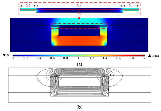
Figure 7.
Magnetic field distribution of the MR damper. (a) Contour of Magnetic flux density. (b) distribution of magnetic flux lines.
Taking into account the uneven distribution of the magnetic field in the damping gaps, to analyze the magnitude of the magnetic flux density in the channel at different positions, an observation path, l1, as shown in Figure 7a, was defined in the gap. The distribution curve of magnetic flux density along the path, as shown in Figure 8, was obtained by simulation. It can be seen from Figure 8a that when the damper was excited to reciprocate, the distribution of the magnetic field in the damping gap was almost unchanged at different positions of the piston, indicating that the position and velocity of the piston head have no obvious influence on the magnitude and distribution of the magnetic field in the damping gap. It can be seen from Figure 8b that when excitation currents of different magnitudes were given, due to structural symmetry, the magnetic flux density in the damping gaps was also symmetrically distributed at the midpoint of the path l1, and the magnetic flux density in the effective damping gaps S1 and S3 were equal in magnitude for each current. In addition, because the excitation coil does not have magnetic permeability, the magnetic flux density dropped sharply in the area close to the excitation coil. Hence, the magnetic flux density of the S2 section approaches zero.
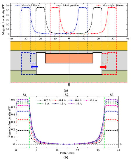
Figure 8.
Distribution of magnetic flux density along the path. (a) Different positions of the damper piston, (b) different excitation currents.
4.3. Simulation Analysis of Flow Field
In the flow field simulation under the action of the magnetic field, the influence of temperature on the rheological effect was not considered, and the MR fluid was regarded as an incompressible fluid. The fluid properties were defined as a non-Newtonian, with viscosity dependent on shear rate and magnetic flux density. The rheological parameters were set according to Equation (35). The distribution law of the flow field in the damper under the action of the magnetic field was analyzed by coupling the magnetic field and the flow field through Equation (27).
The motion equation of the piston head, x, was specified as Asin(2πft), its amplitude, A, as 10 mm, and the frequency, f, as 1 Hz. When the excitation current was 1.0 A, the flow velocity distribution inside the damper at the initial position is shown in Figure 9. Figure 9a is a contour diagram of the flow velocity. It can be seen from the figure that the flow velocity of the MR fluid in the left and right chambers is small, while the flow velocity in the damping gap is large, and the flow velocity at the damping gaps S1 and S3 is more significant than that at the S2 section. This is mainly because the passage area of the S1 and S3 sections is the smallest, so the flow velocity at these two sections is more significant than other areas. At the same time, it can be found that the flow velocity at both ends of the damping gap is distributed like a spray flame, which shows that the flow velocity at the entrance and exit of the gap has a large gradient. Figure 9b is the distribution of flow velocity. It can be seen from the figure that the distribution of flow velocity at the S1 and S3 sections of the damping channel are relatively concentrated, and the contour distribution at the S2 section is relatively uniform, indicating that the flow velocity in the effective damping gap has a wide constant velocity zone. The flow velocity at the S2 section has a certain gradient of change caused by the different distribution of the magnetic field in the three-section damping gap. The magnetic field changes the rheological properties of the MR fluid.
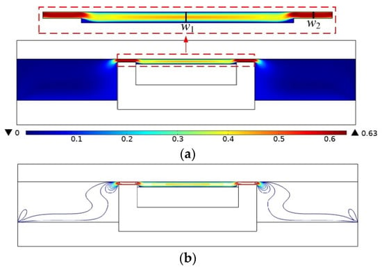
Figure 9.
Velocity distribution of the MR damper. (a) Contour of flow velocity, (b) distribution of flow velocity.
To analyze the flow state of the MR fluid at different positions of the damping gap when the damper is energized, two observation paths w1 and w2 were defined in the gap as shown in Figure 9a, where w1 and w2 are in the center of channels S2 and S3. According to Figure 8b, the magnetic flux density at path w2 is the maximum value in the damping gap, and the magnetic flux density at path w1 tends to zero. The flow velocity and shear rate of the MR fluid were observed along the two paths, and the results are shown in Figure 10. As can be seen from Figure 10a, the velocity of the MR fluid at path w1 presents a parabolic distribution, which is the same as that of a Newtonian fluid. The velocity reaches a maximum in the middle and tends to zero at both ends. As can be seen from Figure 10b, the MR fluid flows in the plunger mode at path w2, and the velocity in most of the middle section is almost the same. The area where the fluid shear rate is close to zero is called the plunger area. Comparing the two figures, it can be seen that the plunger area where the MR fluid flows at path w2 is much broader than that at path w1. The large magnetic flux density causes the rheological effect of the MR fluid under the action of a magnetic field, and its viscosity and shear yield stress will increase sharply, resulting in the broader flow plunger area. The magnetic flux density at path w1 tends to zero, where the MR fluid appears as a Newtonian fluid state with minimal viscosity and yield stress. Hence, its flow plunger area is very narrow.
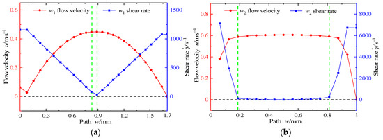
Figure 10.
Flow state of MR fluid along the path. (a) Path w1, (b) path w2.
Figure 11 shows the distribution of dynamic viscosity inside the damper under different currents at the initial position. It can be seen from the figure that the dynamic viscosity in the damping gaps S1 and S3 is much larger than in other areas, and it increases with the current. This is because there is a strong magnetic field in the gaps S1 and S3. The magnetic flux density varies as the current increases. The MR fluid changes from a Newtonian fluid state to a semi-solid state under the magnetic field. The yield stress of its flow increases rapidly according to Equation (35), and the combination of Equation (25) shows that an increase in the yield stress will lead to an increase in the viscosity of the MR fluid.
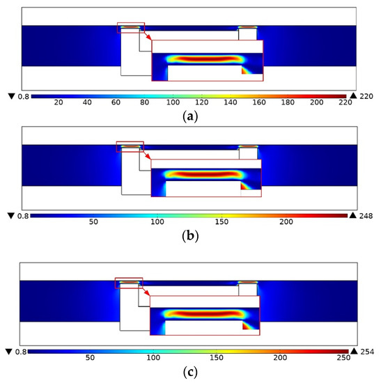
Figure 11.
Dynamic viscosity distribution under different currents. (a) Current of 0.6 A, (b) current of 1 A, (c) current of 1.4 A.
Point p0 on the right boundary of the damper chamber was selected as the pressure reference, that is, the pressure at point p0 was set to zero. The initial position of the pressure distribution in the damper is shown in Figure 12 when the given excitation current was 1.0 A. Figure 12a is a cloud chart of pressure distribution. The pressure distribution in the left and right chambers is relatively uniform, there is a significant pressure difference between the two chambers, and the pressure change gradient along the damping channel is large. Because in the initial position, the piston head will stretch to the left to compress the left chamber, forcing the MR fluid to flow from the left chamber to the right chamber through the damping gap. The MR fluid flowing through the gap will produce a large magnetically induced pressure drop under the magnetic field, resulting in a large pressure difference between the two chambers.
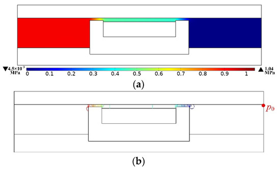
Figure 12.
Pressure distribution of MR damper. (a) Cloud chart of pressure distribution. (b) Contour map of pressure distribution.
Figure 12b is a contour map of pressure distribution. The pressure in the S1 and S3 sections of the damping gap are dense, while the pressure in the S2 section is more minor. The pressure drop caused by the MR fluid flowing through the gaps is mainly concentrated in the two sections of the effective damping gap. Since the magnetic flux density in the S2 section tends to zero, there is only a relatively small amount of viscosity-induced pressure drop when the MR fluid circulates. Hence, the pressure drop it can provide is relatively small.
To analyze the influence of the excitation current on the pressure drop of the MR fluid flowing in the damping gap, we observed the pressure distribution in the gap under different currents along the path l1. The results are shown in Figure 13. It can be seen from the figure that the pressure along the path of the damping gaps S1 and S3 has a large gradient, and its variation range increases with the increase in the excitation current. The pressure at the S2 section has a minor change gradient along the path. The pressure distribution curves under different currents are almost parallel at the S2 section, and the magnitude of the change hardly changes with the current. The damping gap’s S1 and S3 sections have strong magnetic flux density, which will increase with an increase in the excitation current, while the magnetic flux density at the damping gap S2 approaches zero under each current. The strength of the rheological effect of the MR fluid is related to the strength of the magnetic field. The distribution and change of the magnetic field in the gap will eventually result in the pressure distribution along the path as shown in the figure.
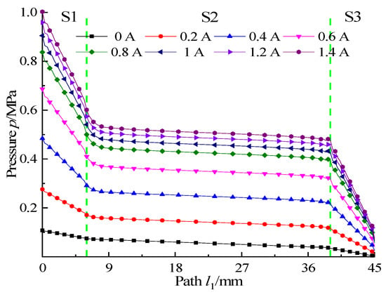
Figure 13.
Pressure distribution along the path at different currents.
4.4. Simulation Analysis of Structural Stress Field
In the simulation of the structural stress field under the action of the magneto–fluid field, the piston head is the core component of the MR damper and can be regarded as a small dynamic deformation body when the damper is working. In the simulation, the force of the structure other than the piston head was not considered. The properties of the piston head area are set to linear elasticity, and its Young’s modulus, poisson’s ratio, and density are all derived from the materials in the library. At the same time, the displacement equation of the piston head subjected to sinusoidal excitation is specified by the dynamic mesh as x = Asin(2πft), and the boundary load on the piston head is defined as the pressure, p, of the MR fluid. The fluid–solid coupling boundary is boundary 1, shown in Figure 6. When the amplitude of the sinusoidal reciprocating movement of the piston head, A, was 10 mm and the frequency, f, was 1 Hz, the stress distribution of the piston head under different excitation currents is shown in Figure 14. Because the velocity of the sinusoidal motion at the initial position is the largest in the entire period, the figure only shows the stress distribution of the piston head at the initial position under different currents.

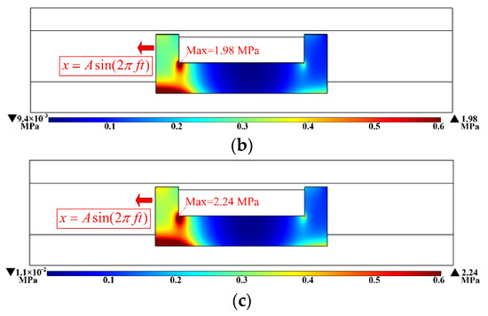
Figure 14.
Stress distribution under different currents of the MR damper. (a) Current of 0.6 A, (b) current of 1 A, (c) current of 1.4 A.
Comparing the three figures, it can be seen that the stress concentration point is located at the corners of the bobbin, and the internal stress of the piston head increases with the increase in the excitation current. An increase in the current will lead to an increase in the pressure difference between the two chambers when the damper moves, which will increase the force of the MR fluid on the piston head and eventually lead to the increase of the stress on the piston head. When the current was 0.6 A, 1 A, and 1.4 A, the maximum internal stress of the piston head was 1.42 MPa, 1.98 MPa, and 2.24 MPa, respectively. The maximum value is far less than the allowable stress of No.10 low carbon steel, which shows that the proposed MR damper is safe during operation.
The sum of the reaction forces of the MR fluid on the piston head is the output damping force of the damper. When the piston head is subjected to a sinusoidal excitation with an amplitude, A, of 10 mm and frequency, f, of 1 Hz, by solving the total reaction force globally, the variation curve of the damper output damping force with displacement under different excitation currents can be obtained, as shown in Figure 15. It can be seen from the figure that the output damping force changes little with the displacement, and its distribution is symmetrical about the relative equilibrium position. However, by comparing the damping force versus displacement curves for each current, it can be seen that the output damping force of the damper will increase with the increase in the excitation current. The main reason is that the increase of the current will increase the magnetic flux density in the damping gap. The total reaction force of the MR fluid on the piston head can be divided into two parts: magnetically induced and viscosity-induced damping force. The increase in the magnetic field will increase the magnetic damping force, making output damping force larger. At the same time, due to the magnetic saturation of the damper, the output damping force increase becomes lower with the increase in current when the current reaches 1 A. The output damping force and dynamic range of the MR damper are the main indices to evaluate its dynamic performance. The ratio of the output damping force to the viscosity-induced damping force is the dynamic range of the proposed damper. The dynamic range is 1 when the current is 0 A. There is only viscous damping force in the damper, and its magnitude is 124.8 N. When the current is 1.4 A, the output damping force of the damper is up to 1134.6 N and the dynamic range is up to 9.1. The simulation results show that the proposed damper can output appropriate damping force and has a wide adjustment range of damping force, which meets the requirements of an automobile shock absorber.
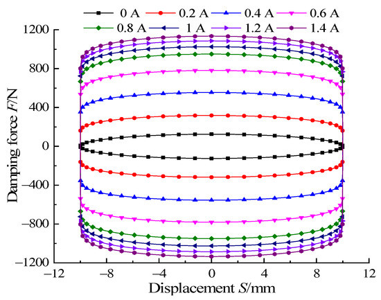
Figure 15.
Damping force versus displacement at different currents.
To study the influence of different vibration excitations on the output damping force of the damper, keeping the current constant at 1 A, sinusoidal excitations of different frequencies and amplitudes for the piston head, and the dynamic simulation results are shown in Figure 16. Figure 16a is the relationship curve of output damping force with displacement at different frequencies when the amplitude is 10 mm. Figure 16b is the relationship curve of output damping force with displacement under different amplitudes when the frequency is 1 Hz. At the same amplitude, the output damping force increased slightly with an increase in the frequency; and at constant frequency, the output damping force increased slightly with an increase in amplitude. The main reason is that when a certain excitation current was given, the proposed damper has both viscous and magnetically induced damping forces under the action of the magnetic field. The magnetically induced damping force is only related to the excitation current, and the current does not change, therefore, the magnetically induced damping force is constant. The viscosity-induced damping force is related to the flow velocity of the MR fluid; the faster the velocity, the greater the viscous damping force. As the excitation frequency and amplitude of the piston head increase, the flow velocity of the MR fluid in the damper will increase, increasing the viscosity-induced damping force, and the viscosity-induced damping force accounts for a smaller proportion of the total damping force. Therefore, the output damping force of the damper will increase slightly with frequency and amplitude.
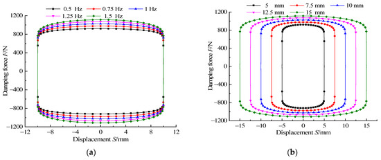
Figure 16.
Damping force versus displacement at different sinusoidal excitation at (a) different frequencies and (b) different amplitudes.
5. Experimental Analysis of Proposed MR Damper
5.1. Damping Performance Test System
To test the dynamic performance of the proposed MR damper and verify the accuracy of the multiphysics coupling simulation, a damper prototype, as shown in Figure 17, was fabricated according to the structural size parameters in Table 1, and the dynamic performance test rig, as shown in Figure 18, was also built.
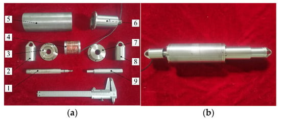
Figure 17.
Prototype of MR damper. (a) Components: (1) left piston rod, (2) left lifting lug, (3) left end cover, (4) piston head, (5) cylinder, (6) end shield, (7) right end cover, (8) right lifting lug, (9) right piston rod. (b) the prototype.
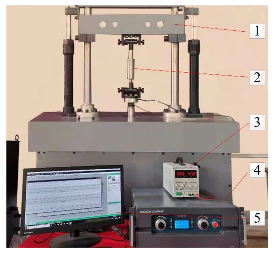
Figure 18.
Dynamic performance test rig. (1) Vibration excitation platform, (2) MR damper, (3) DC power, (4) electro-hydraulic servo controller, (5) computer.
Figure 18 shows that the test system was composed of a vibration excitation platform for the damper, the proposed MR damper, a DC power supply, an electro-hydraulic servo controller and a computer. One end of the MR damper was fixed on the beam of the bench and the other end was connected to the power rod of the vibration excitation platform. The DC power supply was used to provide the proposed damper with different excitation currents. The electro-hydraulic servo controller was connected to the vibration excitation platform for data transmission, conversion, and driving the hydraulic servo valve, and controlled the vibration excitation platform to drive the damper to make the corresponding vibration x(t). The computer is connected to the electro-hydraulic servo controller to run the control program and obtain the feedback output signal. In the computer, the vibration frequency and amplitude of the vibration bench can be set by the program, and different displacement signals can be applied to the damper. The force and speed sensors were built into the test bench to collect the speed, position, and output damping force information of the magnetorheological damper under each working state in real-time and feed them back to the computer.
5.2. Damping Performance Analysis
To test the influence of different currents on the output damping force of the proposed damper, the amplitude of the sinusoidal motion of the vibration excitation platform was set to 10 mm, and the frequency was 1 Hz. At the same time, considering the weight of the damper, the test system was debugged. The DC power is adjusted to provide different excitation currents to the damper. The experiment measured the relationship curve between output damping force and displacement under different currents, as shown in Figure 19. It can be seen from the figure that the output damping force of the damper varies slightly with displacement. The tiny zigzags appearing on the curve were mainly caused by signal interference and weak vibration during the experiment. Comparing the damping force and displacement curves under different currents, as the excitation current increases, the output damping force of the damper will also increase. In addition, the simulation and the experiment have the same growth trend. When the excitation current reaches 1 A, the output damping force measured by the experiment also slows down with the increase of the current, which verifies that the damper in this condition is close to the magnetic saturation state.
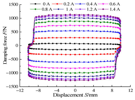
Figure 19.
Damping force versus displacement at different currents.
When the current was 0 A, the dynamic range was 1, the damper has only viscosity-induced damping force, and its magnitude is 119.1 N. When the current was 1.4 A, the measured output damping force reached 1200 N, and the dynamic range reached 10.1. Experimental results show that the proposed damper can output appropriate damping force and has a wide dynamic range, which meets the requirements of automotive shock absorbers.
To test the influence of external vibration excitation changes on the output damping force of the proposed damper, the output current of the DC power was kept constant at 1 A, and the working frequency and amplitude of the vibration excitation platform were changed to apply different sinusoidal displacements to the damper. The variation curve of the output damping force under different sinusoidal excitation is shown in Figure 20. Figure 20a is the relationship curve of output damping force with displacement at different frequencies when the amplitude is 10 mm; Figure 20b is the relationship curve of output damping force with displacement under different amplitudes when the frequency was 1 Hz. Under the same amplitude, the output damping force increased slightly with the increase in frequency; at the same frequency, the output damping force increased slightly with the rise in amplitude.
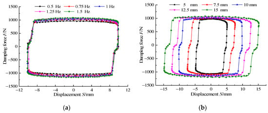
Figure 20.
Damping force versus displacement at different sinusoidal excitation at (a) different frequencies and (b) different amplitudes.
To verify the accuracy of the multiphysics coupling simulation, we compared the output damping force simulation values and the experimental values of the designed damper at applied currents of 0.2 A, 0.6 A, 1 A, and 1.4 A, and the results are shown in Figure 21. The damping force to displacement relationship measured in the experiment has the same variation law as that in the simulation, but the curves obtained in the experiment are not completely in the regular square distribution as in the simulation. There are different degrees of deformations at the maximum strokes of stretching and compression. The main reason lies in the fact that the MR fluid in the damper was not completely perfused during the experiment, resulting in a certain volume of air mixed into the chamber, which caused a small segment of empty path in the process of tension and compression of the damper due to the inability to compensate for the missing liquid in the chamber in time. Therefore, the displacement curves of damping force are somewhat missing. Comparing the simulation values of the output damping force with the experimental values shows that the output damping force obtained by the simulation can approximate the experiment under different currents. The comparison result verifies the accuracy of the multiphysics coupling simulation.
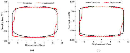
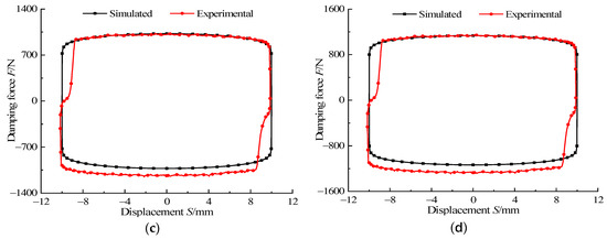
Figure 21.
Comparison between simulated and experimental damping force under different currents. (a) Current of 0.2 A, (b) current of 0.4 A, (c) current of 0.1 A, (d) current of 1.4 A.
In order to further verify the accuracy of the multiphysics coupling simulation, the dynamic performance index was measured experimentally and the damper was compared with the simulation. The results were shown in Figure 22. The output damping force and the dynamic range measured experimentally under different currents had constant changing trends in the simulation, and the simulation value was only slightly smaller than the experimental value. Due to the machining accuracy and assembly errors of the damper, the internal friction of the damper was increased, making the experimental value of the damping force greater than the simulation value. At the same time, due to the measurement error, there will be an error between the experimental value and the simulation value. When the current was 1.4 A, the output damping force and dynamic range obtained by simulation were 1134.6 N and 9.1, the output damping force and dynamic range measured by experiment were 1200.0 N and 10.1. The damping force error between the simulation and experiment was only 5.5%, and the dynamic range error between the simulation and experiment was only 9.9%. By comparing the simulation results with the experimental results, the accuracy of the multiphysics coupling simulation was verified.
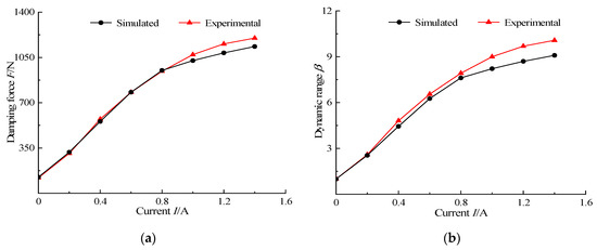
Figure 22.
Simulated and experimental comparison of dynamic performance. (a) Comparison of damping forces under different currents, (b) comparison of dynamic range under different currents.
6. Conclusions
According to the requirements of a shock absorber for automobile suspension, a double-rod MR damper under shear and valve mode was designed. The mechanical model, electromagnetic field model, flow field model, and structural stress field model of the proposed damper were deduced and established.
Considering the non-Newtonian constitutive relationship of the MR fluid, a multiphysics coupling simulation model of the MR damper was established using COMSOL software, and the coupling analysis of the three fields was carried out. The static magnetic field characteristics, dynamic flow field characteristics, stress distribution and dynamic performance of the proposed damper under the action of multiphysics coupling were obtained by simulation. The simulation results confirm the feasibility of the damper structure design.
When the current was 1.4 A, the damping force and dynamic range of simulation were 1134.6 N and 9.1, respectively. The damping force and dynamic range of the experimental damper were 1200.0 N and 10.1, respectively. The damping force error between the simulation and the experiment was only 5.5%, and the dynamic range error between the simulation and the experiment was only 9.9%. By comparing simulation and experimental results and error analysis, the accuracy of the multiphysics coupling simulation in this paper was further verified.
Author Contributions
G.H. contributed the multiphysics coupling of the MR damper and edited the paper; L.W. conducted the experimental research and wrote the first draft. Y.D. designed the MR damper and carried out the theoretical analysis. L.Y. supported the experimental process. B.L. revised the paper. All authors have read and agreed to the published version of the manuscript.
Funding
This research was funded by the National Natural Science Foundation of China, grant number 51765016.
Conflicts of Interest
The authors declare no conflict of interest.
References
- Shiao, Y.; Kuo, W.H.; Nguyen, Q.A.; Lai, C.W. Development of a variable-damping magnetorheological damper with multiple poles. J. Vibroeng. 2015, 17, 1071–1078. [Google Scholar]
- Bai, X.-X.; Hu, W.; Wereley, N.M. Magnetorheological Damper Utilizing an Inner Bypass for Ground Vehicle Suspensions. IEEE Trans. Magn. 2013, 49, 3422–3425. [Google Scholar] [CrossRef]
- Floreán-Aquino, K.H.; Arias-Montiel, M.; Linares-Flores, J.; Mendoza-Larios, J.G.; Cabrera-Amado, Á. Modern Semi-Active Control Schemes for a Suspension with MR Actuator for Vibration Attenuation. Actuators 2021, 10, 22. [Google Scholar] [CrossRef]
- Cho, C.H.; Choi, S.B. Designing Requirement of Spring and MR Damper for New Type Baby Car Seat. Appl. Mech. Mater. 2015, 741, 28–31. [Google Scholar] [CrossRef]
- Hu, G.; Liu, Q.; Ding, R.; Li, G. Vibration control of semi-active suspension system with magnetorheological damper based on hyperbolic tangent model. Adv. Mech. Eng. 2017, 9, 1–15. [Google Scholar] [CrossRef]
- Yang, J.; Ning, D.; Sun, S.; Zheng, J.; Lu, H.; Nakano, M.; Zhang, S.; Du, H.; Li, W. A semi-active suspension using a magnetorheological damper with nonlinear negative-stiffness component. Mech. Syst. Signal Process. 2021, 147, 107071. [Google Scholar] [CrossRef]
- Dong, X. Design and characterization of axial flux permanent magnet energy harvester for vehicle magnetorheological damper. Smart Mater. Struct. 2015, 25, 015024. [Google Scholar] [CrossRef]
- Sun, S.; Tang, X.; Yang, J.; Ning, D.; Du, H.; Zhang, S.; Li, W. A New Generation of Magnetorheological Vehicle Suspension System with Tunable Stiffness and Damping Characteristics. IEEE Trans. Ind. Inform. 2019, 15, 4696–4708. [Google Scholar] [CrossRef]
- Tang, X.; Du, H.; Sun, S.; Ning, D.; Xing, Z.; Li, W. Takagi–Sugeno Fuzzy Control for Semi-Active Vehicle Suspension with a Magnetorheological Damper and Experimental Validation. IEEE/ASME Trans. Mechatron. 2016, 22, 291–300. [Google Scholar] [CrossRef]
- Sassi, S.; Sassi, A.; Cherif, K.; Tarlochan, F. Magnetorheological damper with external excitation for more efficient control of vehicles’ dynamics. J. Intell. Mater. Syst. Struct. 2018, 29, 2919–2932. [Google Scholar] [CrossRef]
- Satria, R.R.; Ubaidillah, U.; Imaduddin, F. Analytical Approach of a Pure Flow Mode Serpentine Path Rotary Magnetorheological Damper. Actuators 2020, 9, 56. [Google Scholar] [CrossRef]
- Zhang, X.; Li, Z.; Guo, K.; Zheng, F.; Wang, Z. A novel pumping magnetorheological damper: Design, optimization, and evaluation. J. Intell. Mater. Syst. Struct. 2017, 28, 2339–2348. [Google Scholar] [CrossRef]
- Kim, K.; Chen, Z.; Yu, D.; Rim, C. Design and experiments of a novel magneto-rheological damper featuring bifold flow mode. Smart Mater. Struct. 2016, 25, 075004. [Google Scholar] [CrossRef]
- Li, G.; Yang, Z.-B. Modelling and Analysis of a Magnetorheological Damper with Nonmagnetized Passages in Piston and Minor Losses. Shock. Vib. 2020, 2020, 1–12. [Google Scholar] [CrossRef] [Green Version]
- Ruan, X.; Xuan, S.; Zhao, J.; Bian, H.; Gong, X. Mechanical performance of a novel magnetorheological fluid damper based on squeeze-valve bi-mode of MRF. Smart Mater. Struct. 2020, 29, 055018. [Google Scholar] [CrossRef]
- Yang, Y.; Xu, Z.-D.; Guo, Y.-Q.; Xu, Y.-W.; Zhang, J. Internal magnetic field tests and magnetic field coupling model of a three-coil magnetorheological damper. J. Intell. Mater. Syst. Struct. 2020, 31, 2179–2195. [Google Scholar] [CrossRef]
- Mangal, S.K.; Kumar, A. Experimental and Numerical Studies of Magnetorheological (MR) Damper. Chin. J. Eng. 2014, 2014, 1–7. [Google Scholar] [CrossRef] [Green Version]
- Olivier, M.; Sohn, J.W. Design and geometric parameter optimization of hybrid magnetorheological fluid damper. J. Mech. Sci. Technol. 2020, 34, 2953–2960. [Google Scholar] [CrossRef]
- Ganesha, A.; Patil, S.; Kumar, N.; Murthy, A. Magnetic field enhancement technique in the fluid flow gap of a single coil twin tube Magnetorheological damper using magnetic shields. J. Mech. Eng. Sci. 2020, 14, 6679–6689. [Google Scholar] [CrossRef]
- Golinelli, N.; Spaggiari, A. Experimental validation of a novel magnetorheological damper with an internal pressure control. J. Intell. Mater. Syst. Struct. 2017, 28, 2489–2499. [Google Scholar] [CrossRef] [Green Version]
- Hu, G.; Liu, H.; Duan, J.; Yu, L. Damping performance analysis of magnetorheological damper with serial-type flow channels. Adv. Mech. Eng. 2019, 11, 1–12. [Google Scholar] [CrossRef] [Green Version]
- Li, S.; Meng, W.; Wang, Y. Numerical and experimental studies on a novel magneto-rheological fluid brake based on fluid–solid coupling. Sci. Prog. 2020, 103, 1–33. [Google Scholar] [CrossRef] [Green Version]
- Gurubasavaraju, T.M.; Kumar, H.; Mahalingam, A. An approach for characterizing twin-tube shear-mode magnetorheological damper through coupled FE and CFD analysis. J. Braz. Soc. Mech. Sci. Eng. 2018, 40, 139. [Google Scholar] [CrossRef]
- Gołdasz, J.; Sapiński, B. Application of CFD To Modeling of Squeeze Mode Magnetorheological Dampers. Acta Mech. Autom. 2015, 9, 129–134. [Google Scholar] [CrossRef] [Green Version]
- Mata, G.T.; Kumar, H.; Mahalingam, A. Performance analysis of a semi-active suspension system using coupled CFD-FEA based non-parametric modeling of low capacity shear mode monotube MR damper. Proc. Inst. Mech. Eng. Part D J. Automob. Eng. 2019, 233, 1214–1231. [Google Scholar] [CrossRef]
- Zhang, P.; Lee, K.-H.; Lee, C.-H. Friction behavior of magnetorheological fluids with different material types and magnetic field strength. Chin. J. Mech. Eng. 2015, 29, 84–90. [Google Scholar] [CrossRef]
- Zhang, J.; Song, W.; Peng, Z.; Gao, J.; Wang, N.; Choi, S.-B.; Kim, G.-W. Microstructure Simulation and Constitutive Modelling of Magnetorheological Fluids Based on the Hexagonal Close-packed Structure. Materials 2020, 13, 1674. [Google Scholar] [CrossRef] [Green Version]
- Cheng, M.; Chen, Z.B.; Xing, J.W. Design, Analysis, and Experimental Evaluation of a Magnetorheological Damper with Meandering Magnetic Circuit. IEEE Trans. Magn. 2018, 54, 1–10. [Google Scholar] [CrossRef]
- Hu, G.; Ru, Y.; Li, W. Design and development of a novel displacement differential self-induced magnetorheological damper. J. Intell. Mater. Syst. Struct. 2015, 26, 527–540. [Google Scholar] [CrossRef] [Green Version]
- Hu, G.; Li, L.; Liu, H.; Liu, F. Effects of Winding Cylinder Materials on Dynamic Performances of a New MR Damper. IEEE Access 2020, 8, 87829–87841. [Google Scholar] [CrossRef]
Publisher’s Note: MDPI stays neutral with regard to jurisdictional claims in published maps and institutional affiliations. |
© 2021 by the authors. Licensee MDPI, Basel, Switzerland. This article is an open access article distributed under the terms and conditions of the Creative Commons Attribution (CC BY) license (https://creativecommons.org/licenses/by/4.0/).