Data-Driven Multiscale Analysis of Household Electricity Carbon Emissions in High-Density Residential Area for Low-Carbon Urban Planning

Abstract

Household electricity consumption is a major and growing source of urban carbon emissions in high-density residential area. However, its influencing mechanisms operate across multiple nested spatial scales and are not fully captured by single-scale analyses. Using electricity consumption data and a household survey from 42 high-density communities in Beijing, this study applies a hierarchical linear model (HLM) to examine how spatial form, socioeconomic attributes, and behavioral factors affect household electricity carbon emissions across urban districts, Ten-Minute Living Circles, residential areas, and Individual dwellings. The results indicate that dwelling-level characteristics exert the most direct influence, while residential-area-level spatial morphology provides an important contextual effect. In contrast, Ten-Minute Living Circles indicators show limited direct associations after accounting for hierarchical structure. Several spatial factors influence emissions through cross-level moderating mechanisms rather than isolated effects. These findings provide a data-driven multiscale analytical framework to support low-carbon planning and retrofit strategies in high-density residential area.

1. Introduction

1.1. Research Motivation

At the 2020 United Nations General Assembly, China pledged to achieve carbon peaking by 2030 and carbon neutrality by 2060. In this new era of green and low-carbon development, households—fundamental units of urban socio-economic systems—have become crucial targets for carbon reduction [1]. Studies indicate that over 70% of China’s carbon emissions arise from household consumption, with electricity use for air conditioning, water heating, and lighting as the main contributors [2].

High-density urban residential area, featuring concentrated populations and buildings, face especially urgent carbon reduction challenges. Spatial form has been identified as a critical factor influencing household electricity carbon emissions and a key lever in low-carbon urban planning. However, the mechanisms underlying these emissions remain unclear due to the complex interplay of multiscale factors. Clarifying these mechanisms is essential for effective carbon reduction in urban residential area.

Using a multiscale dataset, this study explores the interactive mechanisms among influencing factors across different spatial scales. The findings are further translated into data-driven low-carbon planning guidelines for high-density residential areas. This approach bridges the gap between academic research on carbon emissions and practical low-carbon urban design.

1.2. Definition of the Study

1.2.1. Scope of the Study

The study focuses on the area east of the Yongding River in Fengtai District, Beijing, which features diverse newly built high-density residential developments. To accommodate multiscale planning strategies, four spatial scales are examined:

(1)

urban district (the eastern Fengtai area),

(2)

Ten-Minute Living Circles, as defined in China’s Code for Planning and Design of Urban Residential Areas, refer to the built environment within residents’ typical daily activity range (Figure 1),

(3)

residential area, and

(4)

individual dwelling.

1.2.2. Object of Study

Household electricity carbon emissions are affected by factors at multiple scales. At the dwelling level, they depend on housing structure, family behavior, and socio-economic characteristics; at higher levels—residential area, living circle, and urban district—they are shaped by broader spatial and environmental conditions. These form a nested structure, where dwelling-level activities are embedded within residential area-level contexts.

1.2.3. Units of Measurement and Carbon Emission Calculations

Previous studies [3] have used indicators such as per capita or per area electricity carbon emissions. Preliminary analysis showed that household electricity carbon emissions best capture the relationship between socio-economic and spatial factors, and this metric is therefore adopted as the dependent variable.

Annual average household electricity carbon emissions (2018–2020) were calculated for several high-density residential area in Fengtai District using the carbon emission coefficient method, based on a North China electricity emission factor of 940 kgCO₂/MWh [4]:

C_ele1 = X_ele1 * EF

where

C_ele1—Annual average household electricity carbon emission (unit: kg CO₂ per household per year)

X_ele1—Household electricity consumption (unit: MWh per household per year);

EF—Carbon emission factor for electricity consumption in Beijing (unit: kgCO₂/MWh).

2. Literature Review

Based on different attributes, the factors influencing household carbon emissions in urban residential area can be categorized into two major types: morphological factors and non-morphological factors. Although non-morphological factors are difficult to influence via planning interventions, their contribution to household carbon emissions exceeds 60% [5]. Therefore, studies on household carbon emissions should fully account for non-morphological factors. Morphological factors have become a focal point in carbon reduction research within the planning field, with substantial evidence demonstrating their impact on household carbon emissions. For instance, the 5D theory [6] divides the morphological factors influencing household carbon emissions into five aspects: density, diversity, design, destination accessibility, and distance to transit. Researchers such as Huang Jingnan [7], Zhang Jie [8], and Wang Weiqiang [9] have explored both morphological and non-morphological factors at various scales, including urban district, surrounding environments of residential area, and residential communities.

At the urban district scale, the primary focus is on non-morphological factors affecting household carbon emissions, which include age structure [10,11], urban economic consumption levels [10,11], population density [12], employment status [3,11], and relevant policies [10,11]. Morphological factors at this scale include green spaces and water bodies [8,13], land use patterns [8,14,15], accessibility to public transportation [13,16], urban compactness, and job-housing balance [15]. For example, Hong Ye [13] suggested that Large Green–Blue Spaces can reduce household carbon emissions by mitigating summer heat in the region, while Du Wupeng [17] confirmed that urban ventilation corridors can alleviate the urban heat island effect.

For the Ten-Minute Living Circles, the consensus in academia is that transportation facilities and land use diversity around residential area significantly affect household transportation carbon emissions [8,9,16]. Hong S [15] further explored how increasing housing density and the diversity of residents’ race and class within the living circle could reduce household heating and electricity carbon emissions. However, the impact of living circle scale factors on household electricity carbon emissions requires further research. Huang Ru [18] suggested that the surrounding environment of residential area influences household electricity carbon emissions by affecting residents’ duration of stay at home, but the effectiveness and pathways of this impact remain unclear. Similarly, Yang Shangguang’s [19] study in Shanghai indicated that the built environment around residential area significantly affects household travel carbon emissions but has little impact on household electricity carbon emissions.

At the residential area and dwelling scale, which are the units for accounting household carbon emissions, the research is relatively abundant. Non-morphological factors at this scale mainly include household characteristics, attitudes, preferences, and usage behaviors of household members. Domestic and international studies [18,20,21] have discussed the impact of urban household characteristics on household carbon emissions, identifying factors such as household income, age structure, household size, education level, and occupation of the head of household as significantly correlated with household carbon emissions. There is controversy regarding the impact of attitudes and usage behaviors on household carbon emissions. Liu Yan [21] argued that consumption preferences and internet usage habits affect household carbon emissions, whereas Ye Hong [22] and others believed that attitudes and preferences do not significantly impact household carbon emissions. Morphological factors at the residential area and dwelling scale primarily include building characteristics and the residential environment. Research [8,12,16] has confirmed that housing building area has a significant positive effect on household carbon emissions, and building characteristics such as shape, orientation, window-to-wall ratio, envelope structure, ventilation design, and heating and air conditioning systems also influence household carbon emissions, although their impact is smaller than that of socio-economic factors [3]. Regarding the residential environment, studies [23] have shown that building layout, road patterns, and green space ratio influence household use of lighting, air conditioning, and heating by affecting the microclimate of the residential area, although the extent of this impact remains contentious.

Despite the extensive research on the factors influencing urban household carbon emissions, there are still controversies regarding the relationship and mechanisms of influence among these factors. These controversies are mainly reflected in the chaotic research scales, the lack of consideration of factors at the urban district and living circle scales, and the incomplete construction of the factor system influencing household carbon emissions. Additionally, existing studies lack control over significant influencing variables and fail to elucidate the interactive effects among influencing factors, leading to a lack of consensus. Therefore, this paper addresses the complexity of factors influencing household carbon emissions in urban residential area by collecting and analyzing multiscale data combining top-down and bottom-up approaches, attempting to construct a multi-level model of influencing factors at different spatial scales for urban household electricity carbon emissions.

3. Research Data and Methods

3.1. Data Sources

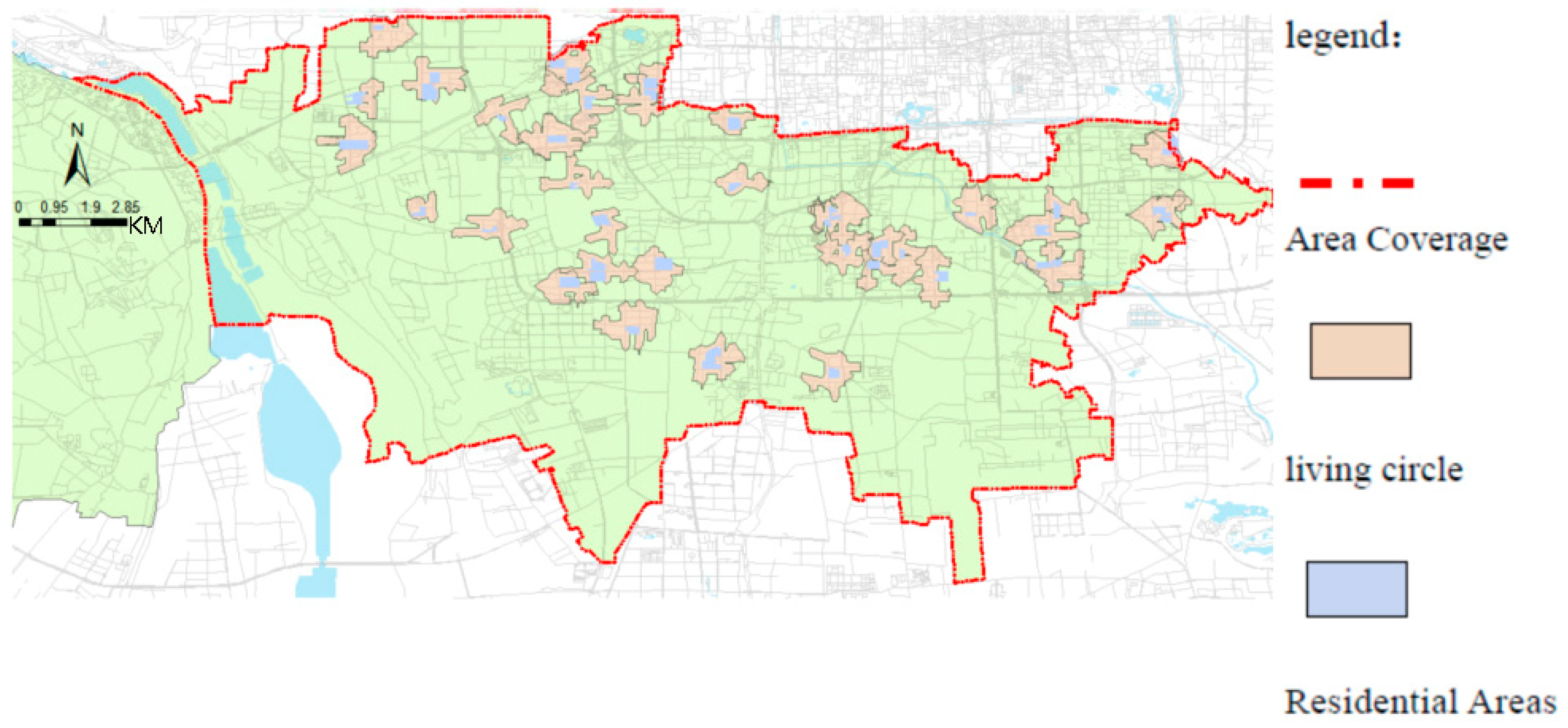
Purposive sampling was adopted in this study to select 42 residential area in eastern Fengtai District, Beijing, ensuring that the samples are representative of high-density urban contexts and diverse spatial morphologies. The eligibility criteria for sample inclusion were as follows:

(1)

Completion after 2000 with stable operation for more than a decade, so as to eliminate confounding effects arising from newly constructed or aging infrastructure;

(2)

A floor area ratio (FAR) greater than 1.8, meeting the definition criteria for high-density residential area;

(3)

Proportionate sampling across five spatial layout types: Point Group Type, Row and Column Type, Mixed Type, Periphery Type, and Free Type (

Table 1. List of research residential area information.

Number	Residential Area Code	Year of Construction	Floor Area Ratio	Total Number of Households	Land Area	Building Area (m2)	Green Space Ratio	Building Density	Combination Form
1	A1	2006	1.9	1723	140,000	260,000	35%	0.19	Point Group Type
2	A2	2003	2	1632	70,000	140,000	35%	0.18
3	A3	2006	2.4	2469	120,000	288,000	35%	0.15
4	A4	2002	2.7	552	25,000	67,500	38%	0.16
5	A5	2000	2.1	828	43,000	90,000	25%	0.22
6	A6	2002	2	1206	49,500	99,000	27%	0.20
7	A7	2003	2.8	1652	80,000	220,000	35%	0.18
8	A8	2013	2	2150	130,000	260,000	30%	0.16
9	B1	2010	2.8	4160	150,000	420,000	42%	0.17	Row and Column Type
10	B2	2008	1.8	977	77,000	140,000	35%	0.22
11	B3	2007	1.9	1471	69,778	132,578	40%	0.19
12	B4	2004	2.1	2101	750,000	160,000	40%	0.19
13	B5	2010	1.9	3617	111,400	236,500	30%	0.19
14	B6	2005	2.3	2620	107,970	250,000	32%	0.20
15	B7	2007	2.5	1580	68,800	172,000	34%	0.11
16	B8	2006	2.6	1116	33,800	87,880	30%	0.24
17	B9	2006	2.4	1709	57,630	138,300	36%	0.19
18	B10	2004	2.4	1873	99,000	245,000	31%	0.22
19	B11	2003	2.6	1350	60,800	160,202	36%	0.23
20	B12	2001	2.5	442	27,344	68,000	30%	0.10
21	B13	2006	2.6	2541	100,000	336,000	31%	0.21
22	B14	2004	2.7	689	23,900	66,000	33%	0.30
23	B15	2009	2.2	2533	97,000	210,000	35%	0.15
24	C1	2004	2.4	2846	120,000	300,000	40%	0.21	Mixed Type
25	C2	2001	2.2	1652	63,660	140,052	35%	0.18
26	C3	2006	2.5	1777	100,250	250,626	35%	0.16
27	C4	2005	2.0	1804	98,298	196,596	46%	0.18
28	C5	2008	2.5	1240	36,400	91,000	30%	0.12
29	C6	2002	2.6	1540	66,780	173,628	30%	0.12
30	C7	2002	2	1501	53,600	134,000	37%	0.15
31	D1	2003	2.1	920	35,100	73,710	40%	0.14	Periphery Type
32	D2	2010	2.6	2183	68,150	177,190	35%	0.20
33	D3	2004	2.2	812	22,304	49,068	30%	0.22
34	D4	2006	2.6	1469	71,799	186,677	32%	0.14
35	D5	2004	2.8	1575	64,400	23,000	33%	0.20
36	E1	2001	2	2253	132,000	264,000	35%	0.27	Free Type
37	E2	2009	2.5	516	24,200	60,500	30%	0.19
38	E3	2008	2.5	1488	72,000	180,000	33%	0.15
39	E4	2003	2.6	2163	90,000	240,000	33%	0.18
40	E5	2006	2.6	1077	37,500	100,000	35%	0.15
41	E6	2001	2.8	988	28,000	80,000	30%	0.24
42	E7	2006	2.8	1723	71,640	200,592	34%	0.15
Schematic layout	Point Group Type		Row and Column Type		Periphery Type		Free Type		Mixed Type

).

This study has certain sampling biases, specifically reflected in the following aspect: the geographic scope of the samples is confined to eastern Fengtai District, which may limit the generalizability of the research findings to other urban districts. Household electricity consumption data (2018–2020) were derived from two sources:

(1)

monthly records provided by the local power department for each building and floor, and

(2)

on-site surveys collecting information on household energy use, spatial form, and socio-economic characteristics (

Table 2. List of socio-economic factors.

Socio-Economic Factor	Mode	Standard Deviation	Minimum	Maximum
Population Size	3	1.1	1	5
Family Structure	Two generations	–	Single living alone	Three generations
Education Level	University	–	High school or below	Master’s
Income Level (CNY)	100,000–200,000	–	100,000–200,000	500,000–1,000,000
Daily Routine	Someone present after work/school	–	Rarely anyone present	Someone present all day

).

Household sampling followed proportional stratified random sampling to ensure representativeness: at least 5% of households in each residential area were surveyed, with samples distributed across all buildings and four floor-level strata (1–6F, 7–11F, 12–18F, >19F).

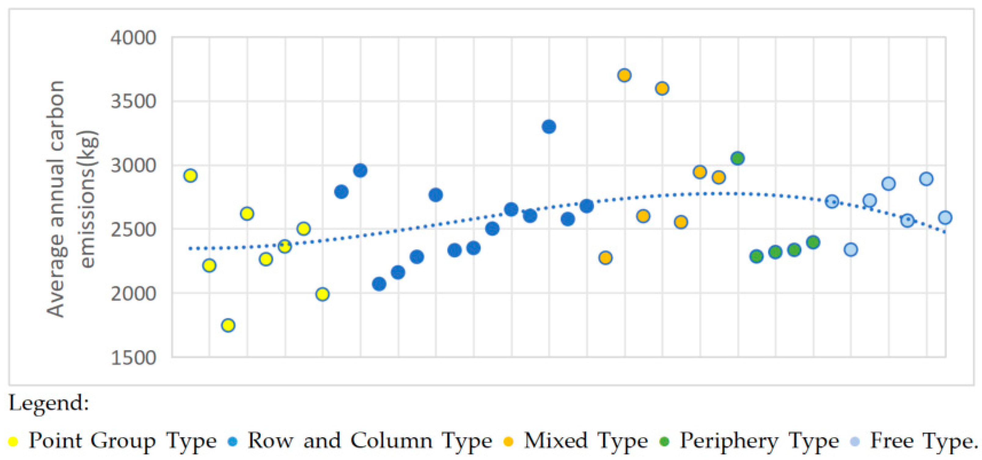
From May to August 2021, household surveys and public-space interviews were conducted, yielding 4300 responses, of which 3642 were valid, corresponding to an effective response rate of 85%. Data obtained from the power grid indicate that the average annual household electricity carbon emissions in high-density residential area of Beijing from 2018 to 2020 were 2592 (kg CO₂ per household per year). By comparison, the on-site household surveys conducted in 2020 recorded an average annual electricity-related carbon emission of 2662 (kg CO₂ per household per year) (

Table 3. List of carbon emission data of research subjects.

	Sample Residential Area (Average Household Carbon Emissions from Electricity Use in 2018–2020 (kg/Household))	Sample Households (Carbon Emissions from Household Electricity Use in 2020 (kg/Household))
average	2592	2662
standard deviation	408	1136
maximum	3698	4650
minimum	1746	1100

). The close correspondence between these two values suggests that household electricity carbon emissions in 2020 did not exhibit abnormal fluctuations relative to the preceding years. This comparison provides a robustness check at the residential area level and supports the reliability of using 2020 household-level electricity carbon emissions as the dependent variable in the analysis.

3.2. Sample Refinement and Characteristic Analysis of Household Electricity Carbon Emissions

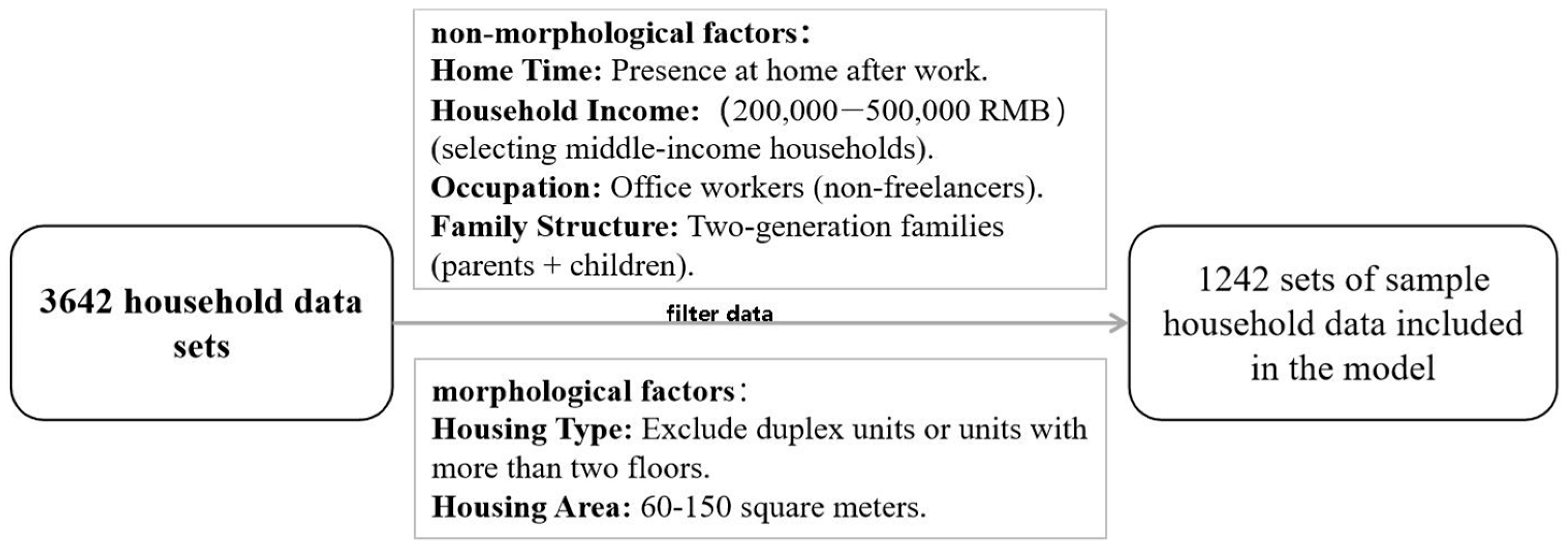
This study focuses on household electricity carbon emissions reducible via spatial planning and design interventions. Following Ye, H [22], we introduced the “standard family” concept, defining it by core indicators including home-stay duration and income (Table 2, Figure 2). To ensure sample homogeneity and carbon emission data authenticity, 1446 ineligible samples were excluded: 892 non-permanent households (unstable electricity consumption characteristics), 321 households with abnormal electricity consumption identified via the three-standard deviation method (to avoid interfering with model estimation), and 233 shared-rental households (ambiguous electricity cost accounting boundaries). From the remaining 2196 samples, two-dimensional screening was conducted: non-morphological screening selected two-generation households with annual income of 200,000–500,000 RMB and office-worker members, excluding 480 samples to retain 1716; morphological screening excluded duplex/multi-story units and those with floor area outside 60–150 m², removing 474 samples, with 1242 final samples included in hierarchical linear model (HLM) analysis.

These households’ electricity consumption is directly affected by morphological factors, avoiding interference from extreme groups. As the mainstream permanent households in the study area, they render the conclusions representative and instructive. Notably, the conclusions have limited applicability to elderly single-person, extremely low-income, and three-generation households. Future research can expand sample coverage to develop a more generalizable model.

Of the original 3642 households, 1242 satisfied the predefined standard family criteria and were thus retained for subsequent hierarchical linear model (HLM) analyses; the average electricity carbon emission level of this refined subsample is presented in Figure 3. To rigorously evaluate whether the sample refinement procedure introduced selection bias into the core outcome variable (household electricity carbon emissions), an independent-samples t-test was performed to compare emission levels between the full sample and the refined subsample. Statistical results indicated no significant difference between the two groups (t = −0.67, p > 0.05), confirming that the screening process did not exert a statistically meaningful impact on the core outcome variable (

Table 4. Descriptive statistics of annual electricity consumption.

	Group	Sample Size (n)	Mean	Standard Deviation (SD)	T
household electricity carbon emissions	the screened subsample	1242	2638	1079	−0.67
	the full sample	3642	2662	1136
house area	the screened subsample	1242	97.29	27.53	−1.79
	the full sample	3642	99.03	34.80

).

3.3. Theoretical Basis and Research Methods

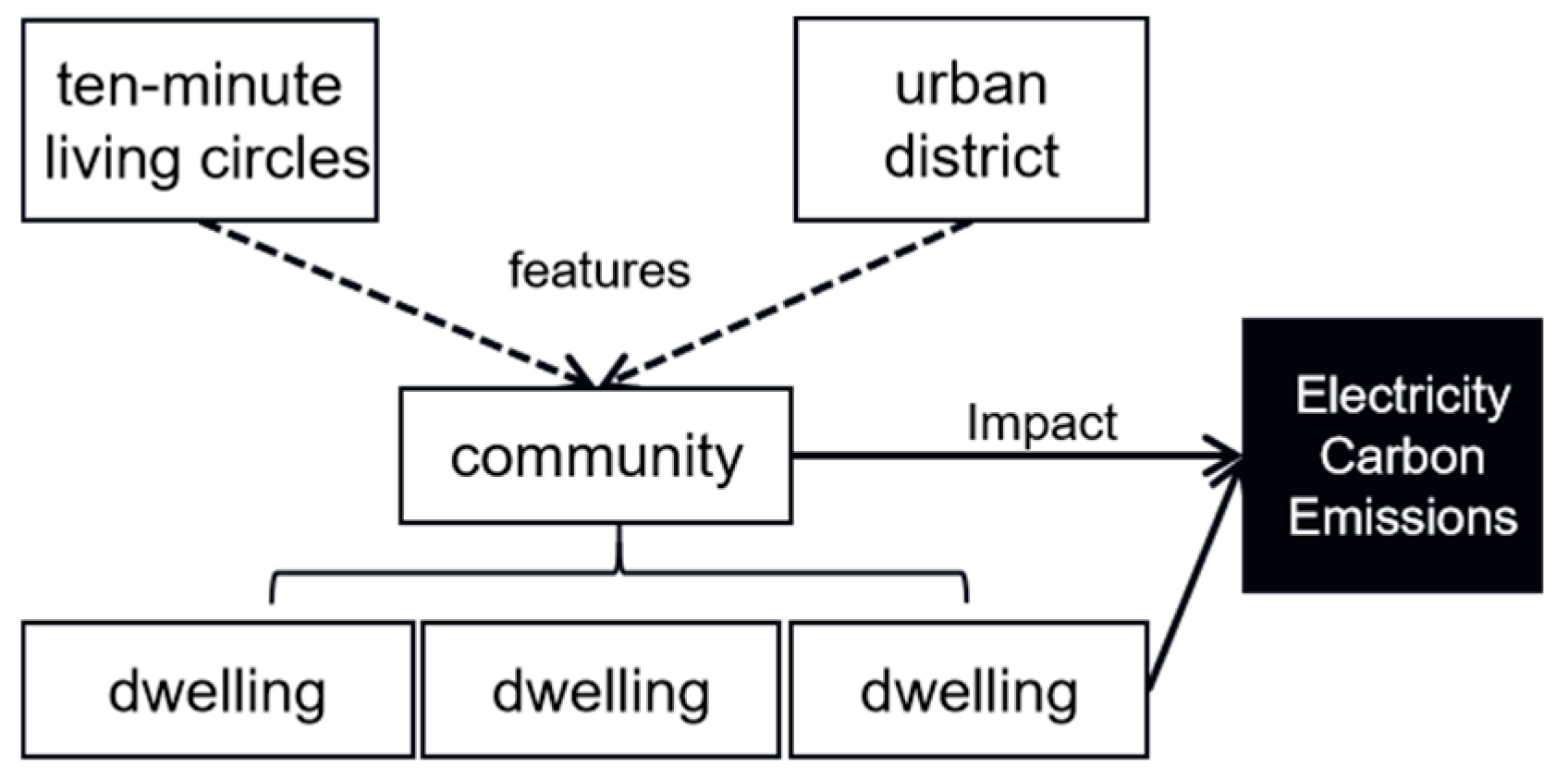
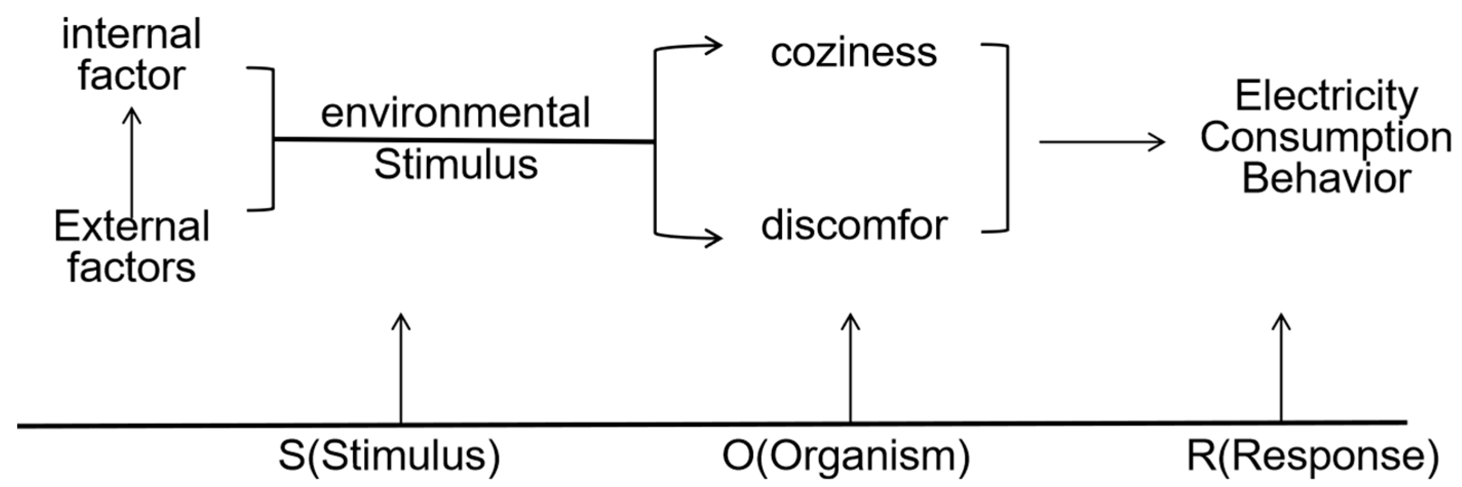
The Stimulus–Organism–Response (S–O–R) framework underpins this study by linking environmental stimuli to residents’ perceptions and everyday practices, which in turn shape electricity-use behavior and its associated carbon emissions [24]. In our context, internal stimuli operate at the dwelling level (e.g., household structure, lifestyle and behavioral patterns, and economic conditions) and directly determine electricity demand. External stimuli arise from broader spatial contexts, including the residential area. Ten-Minute Living Circle environments and district context, such as spatial morphology, land-use functions, and climatic or microclimatic conditions. These contextual factors influence household electricity consumption indirectly by shaping the built environment and thermal comfort. Because electricity-related carbon emissions are jointly driven by factors across nested spatial scales, single-level analyses may obscure contextual effects and cross-level heterogeneity. We therefore adopt a multilevel analytical framework to estimate both household-level and contextual influences within a unified hierarchical structure (Figure 4 and Figure 5).

3.4. Variable Design, Screening, and Model Specification

Based on a comprehensive review of the household carbon emissions literature and in-depth analysis of survey and interview data, this study initially identified a broad set of potential factors influencing household electricity carbon emissions. Variable selection was guided by theoretical relevance, empirical support in prior studies, and data availability, resulting in a multilevel indicator system spanning the dwelling, residential area, Ten-Minute Living Circles, and urban district scales (

Table 5. Explanation and quantification standards of influencing factors for household electricity carbon emissions.

Influencing Factor	Specific Explanation and Quantification Standard
Average Building Shape Coefficient	The average of the shape coefficients of all buildings in the residential area. A higher value indicates poorer average thermal performance of the buildings.
Spatial Openness Variation Coefficient	Represents the layout form of open spaces in the residential area. It refers to the variability in the distance from any point in the open space to the nearest residential building surface.
Public Transport Convenience	Determined by the number of public transport stations within a Ten-Minute Living Circles of the residential area and the distance from these stations to the nearest entrance of the residential area [25].
Surface Temperature. (The land surface temperature data in this study were derived from the Landsat 8 satellite remote sensing images captured over the study area in 2020, and high-resolution Google remote sensing images with a spatial resolution of 2 m were incorporated as auxiliary base maps to support the inversion of land surface temperature. The land surface temperature inversion was conducted using the mono-window algorithm based on ENVI 5.3 software.)	Retrieved using atmospheric correction method.
Urban Functional Zone of the residential area	Divided into core functional zone, science park, ecological functional zone, and general functional zone according to the city’s master plan and current situation.
Ventilation Corridor	The residential area is affected by ventilation corridors if it is within 500 m from the centerline of the main ventilation corridor or within 260 m from the secondary ventilation corridor [17].
Large Green–Blue Spaces	Calculated by the area of green spaces and water bodies larger than 4.55 hectares within a 1.7 km radius of the residential area, representing the influence of Large Green–Blue Spaces [26,27].

and

Table 6. Preliminary screening of variables based on correlation analysis for household electricity carbon emissions in the HLM model.

	Household Characteristics (Level 1): Influencing Factors of Household Electricity Carbon Emissions
Dwelling scale		Variable Category	Pre-Experiment Significance	Treatment Method
	Housing Ownership	Nominal Variable	Significant Negative Correlation	Included in Level 1 Model
	North–South Ventilation	Ordinal Variable	Significant Positive Correlation	Included in Level 1 Model
	Orientation	Nominal Variable	Not Significant	Included in Level 1 Model
	Building Type	Nominal Variable	Not Significant	Included in Level 1 Model
	Housing Area	Scale Variable	Significant Positive Correlation	Included in Level 1 Model
	Air Conditioning Usage Duration	Scale Variable	Significant Positive Correlation	Included in Level 1 Model
	Total Household Population	Scale Variable	Not Significant	Included in Level 1 Model
	Family Structure	Ordinal Variable	Significant Positive Correlation	Included in Level 1 Model
	Household Income	Ordinal Variable	Significant Positive Correlation	Included in Level 1 Model
	Residential area Characteristics (Level 2): Influencing Factors of Household Electricity Carbon Emissions
Residential area	Average Height	Scale Variable	Not Significant	Excluded
	House Price	Scale Variable	Significant Positive Correlation	Included in Level 2 Model
	Variation Coefficient	Scale Variable	Not Significant	Proposed for Full Model
	Shape Coefficient	Scale Variable	Significant Positive Correlation	Included in Level 2 Model
	Green Space Ratio	Scale Variable	Significant Negative Correlation	Included in Level 2 Model
Ten-Minute Living Circles	Public Service Facility Kernel Density	Scale Variable	Not Significant	Excluded
	Public Service Facility Diversity	Scale Variable	Not Significant	Excluded
	Road Network Density	Scale Variable	Not Significant	Excluded
	Public Transport Convenience	Scale Variable	Not Significant	Excluded
Urban District scale	Surface Temperature	Scale Variable	Significant Positive Correlation	Proposed for Full Model
	Functional Zone	Nominal Variable	Significant Positive Correlation	Control Variable, Sample Screening
	Ventilation Corridor	Ordinal Variable	Not Significant	Excluded
	Large Green–Blue Spaces	Scale Variable	Not Significant	Proposed for Full Model

Note: Variable categories are classifications of variables based on their nature and characteristics, falling into three types: nominal variables (only distinguishable by name/category, no numerical meaning or order), ordinal variables (distinguishable by name/category with an ordered relationship between categories, comparable in size or degree), and scale variables (expressible by numbers, with quantitative meaning and amenable to arithmetic operations).

). Spatial morphological variables were derived from corresponding multiscale spatial datasets.

Prior to hierarchical modeling, candidate variables were screened using Pearson correlation analysis to exclude indicators with weak or unstable associations. Multicollinearity among continuous predictors within each hierarchical level was further assessed using variance inflation factors (VIFs), and all VIF values fell within acceptable ranges (

Table A1. Multicollinearity diagnostic results of variables in HLM model.

Variable Level	Variable	Type	Included in Model	VIF	Tolerance	Collinearity Status
Level 1	Housing Ownership	Nominal	Yes	1.32	0.758	No multicollinearity
Level 1	North–South Ventilation	Ordinal	Yes	1.45	0.69	No multicollinearity
Level 1	Orientation	Nominal	Yes	1.28	0.781	No multicollinearity
Level 1	Building Type	Nominal	Yes	1.3	0.769	No multicollinearity
Level 1	Housing Area	Scale	Yes	1.85	0.541	No multicollinearity
Level 1	Air Conditioning Usage Duration	Scale	Yes	2.1	0.476	No multicollinearity
Level 1	Total Household Population	Scale	Yes	1.78	0.562	No multicollinearity
Level 1	Family Structure	Ordinal	Yes	1.42	0.704	No multicollinearity
Level 1	Household Income	Ordinal	Yes	1.35	0.741	No multicollinearity
Level 2	House Price	Scale	Yes	1.9	0.526	No multicollinearity
Level 2	Shape Coefficient	Scale	Yes	1.72	0.581	No multicollinearity
Level 2	Green Space Ratio	Scale	Yes	1.38	0.725	No multicollinearity
Level 2	Surface Temperature	Scale	Proposed	1.82	0.549	No multicollinearity
Level 2	Large Green–Blue Spaces	Scale	Proposed	1.65	0.606	No multicollinearity

), indicating that severe multicollinearity is unlikely to bias coefficient estimates. While some variables—such as housing area, household income, family structure, and residential area-level housing price—are structurally correlated by nature, these relationships reflect underlying socioeconomic stratification rather than statistical artifacts. Accordingly, a hierarchical linear modeling (HLM) framework was adopted to distinguish within-residential-area household effects from between-residential-area contextual effects.

All continuous dwelling-level variables were grand-mean centered to enhance interpretability and reduce collinearity between main effects and cross-level interaction terms. Group-mean centering was not applied in order to preserve comparability across residential communities. Standardized coefficients are reported to facilitate comparison of effect magnitudes, while model estimation was conducted using centered variables in their original units.

Model specification followed a stepwise strategy, progressing from a null model to random-intercept and random-coefficients models, and finally to the full model. Random slopes were specified only for selected continuous dwelling-level variables with strong theoretical justification and sufficient between-residential area variability, while nominal variables were treated as fixed effects. Variables that led to model instability or reduced interpretability were excluded, and alternative model specifications were tested to assess the robustness of the core results. Model performance was evaluated using changes in variance components, likelihood-based fit statistics, and the stability of parameter estimates.

Model diagnostics were conducted to assess key assumptions of the hierarchical linear model. Residuals at both the dwelling and residential area levels exhibited approximate normality and homoscedasticity, and no influential outliers were identified that substantially affected parameter estimates. These diagnostic results indicate that the assumptions of the HLM are reasonably satisfied for the present analysis.

4. Results

4.1. Baseline Regression Results Prior to Hierarchical Modeling

As a preliminary step, a multivariate regression analysis was conducted to explore the associations between household electricity carbon emissions and candidate influencing factors across multiple spatial scales, without accounting for inter-group differences among residential areas. This baseline analysis serves as an exploratory reference for subsequent hierarchical linear modeling rather than as a basis for causal inference (

Table 7. Overview table of regression analysis of influencing factors for household electricity carbon emissions.

Household Characteristics (Level 1): Influencing Factors of Household Electricity Carbon Emissions
	Regression Coefficient	Standard Deviation	t	p
(Constant)		0.173	27.45	0
Housing Ownership	−0.114 **	0.015	−4.595	0
North–South Ventilation	−0.18 **	0.026	−6.168	0
Orientation	−0.035	0.009	−1.304	0.193
Building Type	0.033	0.018	1.357	0.175
Housing Area	0.467 **	0.036	16.009	0
Air Conditioning Usage Duration	0.175 **	0.011	7.103	0
Total Household Population	0.073	0.018	1.54	0.124
Family Structure	0.158 *	0.025	3.434	0.001
Household Income	−0.069 *	0.012	−2.875	0.004
Residential area Characteristics (Level 2): Influencing Factors of Household Electricity Carbon Emissions
(Constant)		3.7	2.218	0.044
Average Height	0.538	0.011	1.38	0.189
House Price	−0.456 **	0.337	−2.182	0.047
Public Service Facility Kernel Density	−0.389	0.204	−1.584	0.136
Public Service Facility Diversity	0.047	0.341	0.171	0.867
Road Network Density	−0.207	0.271	−0.599	0.559
Public Transport Convenience	0.032	0.045	0.121	0.906
Spatial Openness Variation Coefficient	−0.75	1.092	−2.701	0.117
Average Building Shape Coefficient	0.479 *	1.69	2.453	0.028
Surface Temperature	0.745 *	0.043	2.627	0.02
Green Space Ratio	−0.181 *	1.002	−2.611	0.03

Note: * and ** indicate significance at the 0.05 (two-tailed) and 0.01 (two-tailed) levels, respectively. This table reports baseline regression results without accounting for hierarchical structure. Coefficients are presented for exploratory comparison only; inferential interpretation is based on the subsequent HLM results.

).

At the dwelling level, housing area and air-conditioning usage duration exhibited strong positive associations with household electricity carbon emissions, while north–south ventilation and household income were negatively associated. Several variables, including building orientation and building type, were not statistically significant. Variables representing the Ten-Minute Living Circles showed no significant associations in this single-level framework.

At the residential area and urban district scales, surface temperature, average building shape coefficient, housing price, and green space ratio displayed significant associations with household electricity carbon emissions. However, these results do not distinguish between within-residential-area and between-residential-area effects, and may be affected by spatial clustering and contextual heterogeneity.

Therefore, these regression results are used primarily to motivate the adoption of a hierarchical linear model in the following section, which explicitly accounts for multilevel data structure and cross-scale interactions.

4.2. HLM Model Construction and Adaptation

4.2.1. Null Model

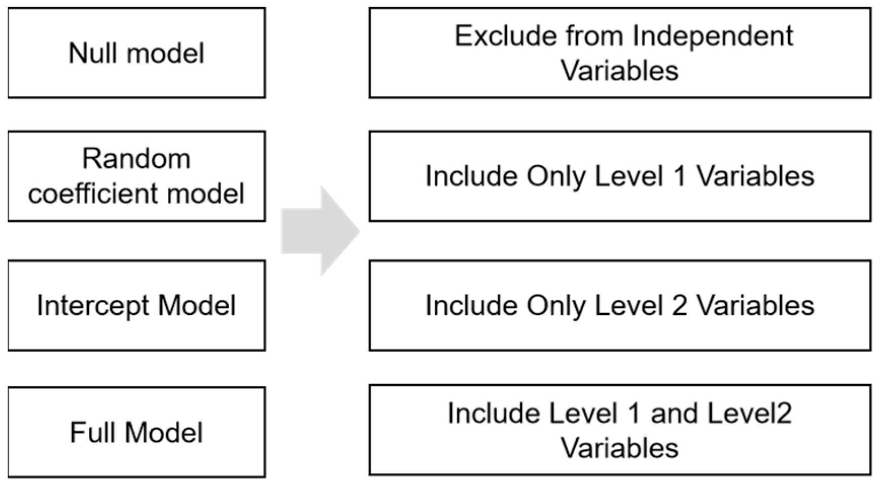
To systematically examine the multilevel determinants of household electricity carbon emissions, hierarchical linear models were constructed sequentially, progressing from a null model to a random coefficients model, an intercept model, and a full multiscale model (Figure 6).

As the first step, a null model was estimated to assess whether household electricity carbon emissions vary significantly across residential area. The intraclass correlation coefficient (ICC) (the intraclass correlation coefficient (ICC) reflects the proportion of variance attributable to differences between levels within the data. Generally speaking, a higher ICC value indicates greater differences between groups and smaller differences within groups, suggesting that the data has a more hierarchical structure. Cohen [28] considered a value greater than 0.059 to indicate the presence of differences between groups) indicates that 37.1% of the total variance is attributable to between residential area differences (

Table 8. Null model parameter statement.

Dependent Variable	τ00	σ2	ICC
household electricity carbon emissions	0.07117	0.12122	0.371

), exceeding the commonly accepted threshold for hierarchical effects. This result confirms the presence of substantial contextual heterogeneity and justifies the use of hierarchical linear modeling.

The null model of HLM for household electricity carbon emissions is as follows:

• Level 1: Y_ij (household electricity carbon emissions) = β_0j + ε_ij
• Level 2: β_0j = γ₀₀ + u_0j

In this model:

β_0j is the Level 1 random intercept.

ε_ij is the Level 1 residual variance.

γ₀₀ is the overall average intercept for the Level 2 random intercept.

u_0j is the residual for the Level 2 random intercept.

4.2.2. Random Coefficients Model

After introducing dwelling-unit-level variables via the stepwise method, the results of the random coefficients model indicated that housing area, air-conditioning usage duration, household income, family structure, building type, and building orientation remained statistically significant (

Table 9. Individual level influencing factors of household electricity carbon emissions considering the impact of residential area characteristics.

	Random Model Coefficients (Regression Analysis Coefficients)	Standard Deviation	t	p
Building Type	0.039 ** (0.033) up	0.013	2.906	0.004
Housing Area	0.254 ** (0.467) down	0.070	3.592	0.001
Air Conditioning Usage Duration	0.218 ** (0.175) up	0.057	3.860	0.000
Family Structure	0.046 ** (0.158) down	0.013	3.682	0.000
Orientation	0.052 * (−0.035) up	0.045	1.827	0.044
Household Income	−0.036 * (−0.069) down	0.020	−1.843	0.045
Housing Ownership	Not significant in initial analysis, not included in the model
North–South Ventilation
Household Population

Note: * and ** indicate significance at the 0.05 (two-tailed) and 0.01 (two-tailed) levels, respectively.

). In contrast to the results of single-level regression, the statistical significance of several variables disappeared, which suggests that their apparent effects can be partially attributed to unobserved heterogeneity at the residential area level. Notably, the inclusion of dwelling-level variables reduced the within-group variance by 44.98%, which greatly improved the model fit and verified the core role of household-level characteristics in explaining household electricity carbon emissions.

Level 1:

• Y_ij (Household Electricity Carbon Emissions) = β_0j + β_1j * (Building Type) + β_2j * (Housing Area) + β_3j * (Air Conditioning Usage Duration) + β_4j * (Family Structure) + β_5j * (Orientation) + β_6j * (Household Income) + ε_ij

Level 2:

• β_0j = γ₀₀ + u_0j β_1j = γ₁₀ β_2j = γ₂₀ + u_1j
• β_3j = γ₃₀ + u_2j β_4j = γ₄₀ β_5j = γ₅₀
• β_6j = γ₆₀ + u_3j

In this model:

β_0j is the Level 1 random intercept.

ε_ij is the Level 1 residual variance.

γ₀₀ is the overall average intercept for the Level 2 random intercept.

u_0j is the residual for the Level 2 random intercept.

4.2.3. Intercept Model

The intercept model only considers the impact of second-level variables on the first-level intercept. In the previous section, we conducted a preliminary analysis of the factors influencing household electricity carbon emissions at the residential area, living circle, and urban district scales based on data from the State Grid Corporation of China. This section’s model, based on survey questionnaire data, assumes no first-level independent variables and uses second-level independent variables (i.e., residential area characteristics) to explain the differences in average household electricity carbon emissions among residential area.

After excluding insignificant influencing factors, the HLM intercept model is as follows:

Level 1:

• Y_ij (Household Electricity Carbon Emissions) = β_0j + ε_ij

Level 2:

• β_0j = γ₀₀ + γ₀₁ * (Total land area) + γ₀₂ * (House Price) + γ₀₃ * (Average Building Shape Coefficient) + u_0j

In this model:

β_0j is the Level 1 random intercept,

Ε_ij is the Level 1 residual variance,

γ₀₀ is the overall average intercept for the Level 2 random intercept,

u_0j is the Level 2 random intercept residual.

The results of the intercept model analysis are similar to the conclusions from the previous correlation analysis. Among all the influencing factors, the residential land area (0.077*), average housing price (0.254*), and average building shape coefficient (0.303**) reached significant levels, while other influencing factors did not show significant effects. This indicates that external carbon emission influencing factors at the residential area level have varying impacts on household electricity carbon emissions. Specifically, the average housing price and average building shape coefficient of the residential area is important influencing factors. After including the aforementioned three influencing factors, the overall intragroup residual decreased by 65.79%, indicating that the introduction of second-level variables has a certain explanatory power for the variation in the first-level intercept.

4.2.4. Full Model

Due to the excessive number of variables in the model, which can lead to non-convergence, the first-level model focuses on key influencing factors at the dwelling scale. To balance model complexity and estimation reliability, the full model prioritized theoretically central dwelling-level variables and introduced higher-level predictors incrementally. This strategy avoids over-parameterization and is consistent with recommended practices for multilevel models with limited higher-level sample sizes. The second-level model continuously introduces new variables while removing insignificant ones and excludes the random effects of nominal variables [29]. The final full model for analyzing the influencing factors of household electricity carbon emissions is as follows:

Level 1:

• Y_ij (Household Electricity Carbon Emissions) = β_0j + β_1j * (Building Type) + β_2j * (Housing Area) + β_3j * (Air Conditioning Usage Duration) + β_4j * (Orientation) + ε_ij

Level 2:

• β_0j = γ₀₀ + γ₀₁ * (Total land area) + γ₀₂ * (House Price) + γ₀₃ * (Average Building Shape Coefficient) + u_0j
• β_1j = γ₁₀
• β_2j = γ₂₀ + γ₂₁ (Average Building Shape Coefficient) + u_2j
• Β_3j = γ₃₀ + γ₃₁ * (House Price) + u_3j
• Β_4j = γ₄₀ + γ₄₁ (Large Green–Blue Spaces)

In this model:

β_0j is the Level 1 random intercept.

ε_ij is the Level 1 residual variance.

γ₀₀ is the overall average intercept for the Level 2 random intercept.

u_0j is the residual for the Level 2 random intercept.

Compared with the null model, the full model shows a significant decrease in both intragroup and intergroup variance, indicating that the model has good explanatory power (

Table 10. Results of HLM analysis of carbon emission impact factors of household electricity consumption.

	Null Model	Random Coefficient Model	Intercept Model	Full Model
γ00	7.865 **	5.527 **	10.084 **	8.324 **
Level 1
Building Type		0.039 **		0.005 *
Housing Area		0.254 **		0.038 **
Air Conditioning Usage Duration		0.218 **		0.223 **
Family Structure		0.046 **
Orientation		0.052 *		0.034 *
Household Income		−0.036 *
Level 2
residential land area			0.077 *	0.065 *
House Price			0.254 *	0.179 *
Average Building Shape Coefficient			0.303 **	0.215 **
House Price * Air Conditioning Usage Duration				0.189 *
Average Building Shape Coefficient * Housing Area				0.057 *
Large Green–Blue Spaces * Orientation				−0.004 *
Intergroup Variance	0.072 **	0.046 **	0.041 **	0.053 **
Level 1 Intragroup Variance	0.123	0.117	0.121	0.043

Note: * and ** indicate significance at the 0.05 (two-tailed) and 0.01 (two-tailed) levels, respectively. Only variables with significant correlations are listed.

).

4.3. Analysis of Key Influencing Factors and Mechanisms of Household Electricity Carbon Emissions

Based on variance decomposition of the hierarchical linear model (HLM), factors operating at different spatial scales exhibit differentiated contributions to household electricity carbon emissions. Dwelling-scale variables explain the largest share of variance, while residential-area-level morphological indicators mainly exert contextual and moderating effects. Urban-district-level factors influence emissions primarily through indirect pathways rather than strong direct coefficients. Only variables that remain statistically significant in the final HLM specification (Table 10) are interpreted as model-derived effects. Other indicators discussed in this section are explicitly treated as model-informed factors, reflecting indirect mechanisms or contextual relevance rather than independent statistical significance.

Given model complexity, only variables with robust statistical significance were retained in the full HLM model. Several indicators—such as urban ventilation corridors, spatial openness variation, and green space ratio—were significant in single-level analyses but not in the multilevel model. Their exclusion reflects weaker independent explanatory power; however, they likely operate indirectly or contextually. Including them in the analysis remains important for understanding the broader environmental conditions shaping household electricity use, as they reveal mechanisms through which urban form and environmental features influence energy consumption, even if their direct effects are absorbed by higher-level contextual factors.

4.3.1. Influencing Factors and Mechanisms at the Urban District Scale

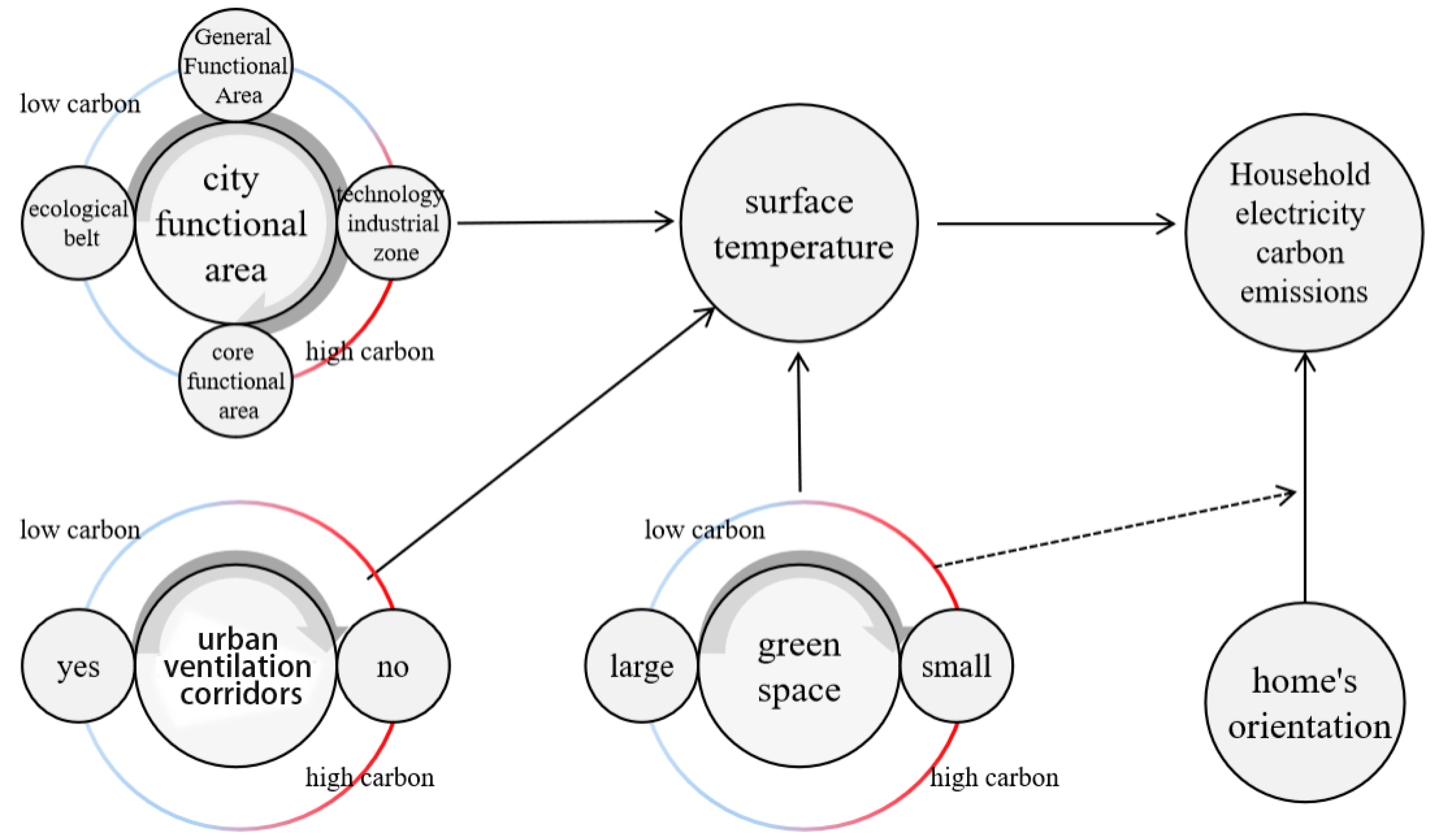
At the urban district scale, the only statistically significant pathway identified in the HLM is the moderating effect of large green and water spaces, which mitigates the impact of unfavorable housing orientation on household electricity carbon emissions. These urban-scale factors primarily operate indirectly or through cross-level interactions rather than strong direct effects, serving as background climatic regulators (Figure 7).

Model-informed factors such as urban ventilation corridors and city functional area were significant in single-level analyses but not retained in the full HLM, suggesting that while their independent explanatory power is limited, they likely influence household electricity use indirectly through microclimatic modulation (e.g., shading, temperature regulation).

Urban ventilation corridors: From an environmental and climatic perspective, urban ventilation corridors are widely recognized for their role in regulating surface temperature and improving outdoor thermal conditions. Existing studies [30] indicate that lower surface temperatures in summer are associated with reduced cooling demand and, consequently, lower household electricity carbon emissions, particularly in regions with hot summers and cold winters. Residential area lacking effective ventilation corridors tend to experience higher surface temperatures [17], which may indirectly increase household electricity consumption for cooling.

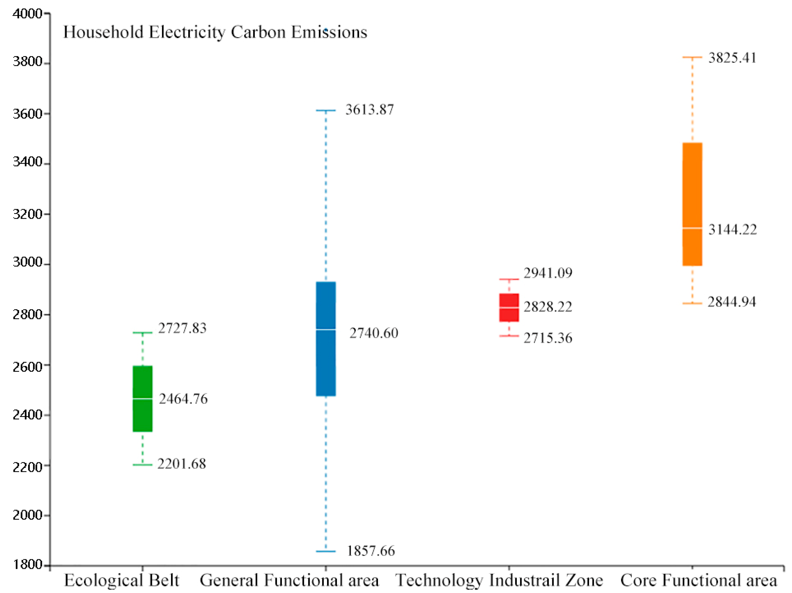
City functional area (Figure 8): Households in ecological development belts, characterized by lower development intensity and more green and water spaces, generally show lower electricity carbon emissions due to favorable microclimates and reduced reliance on indoor cooling and lighting. In contrast, core functional zones have denser, high-intensity development, leading to higher summer surface temperatures and greater cooling demand. At the same time, these areas may benefit from centralized energy systems and agglomeration efficiencies, partially offsetting electricity-related carbon emissions.

4.3.2. Influencing Factors and Mechanisms at Ten-Minute Living Circles

The potential influence of Ten-Minute Living Circles on household electricity carbon emissions in this study is operationalized through indicators capturing public service facility accessibility and transportation convenience around residential areas. Results from the regression analysis and the final HLM consistently indicate that these living-circle indicators do not have statistically significant direct effects on household electricity carbon emissions.

These findings suggest that, within the variable system and multilevel model specification adopted in this study, Ten-Minute-Living-Circle indicators provide limited independent explanatory power for variations in household electricity carbon emissions. One plausible explanation is that the selected indicators primarily reflect external service and transport conditions, which may be only weakly related to household electricity use and associated indoor consumption behaviors. In addition, relatively homogeneous built-environment conditions across high-density residential areas may compress between-area variability in living-circle indicators, thereby reducing their detectable effects in the multilevel framework.

4.3.3. Influencing Factors and Mechanisms at the Residential Area Scale

At the residential area scale, between-group differences account for approximately 37% of the total variance in household electricity carbon emissions, highlighting the contextual role of the residential environment. In the full hierarchical linear model (HLM), the average building shape coefficient, housing price, and total residential land area exhibit the strongest correlations, and are identified as model-derived factors with robust statistical support, which reflect the impacts of development intensity and socio-demographic conditions on household electricity consumption.

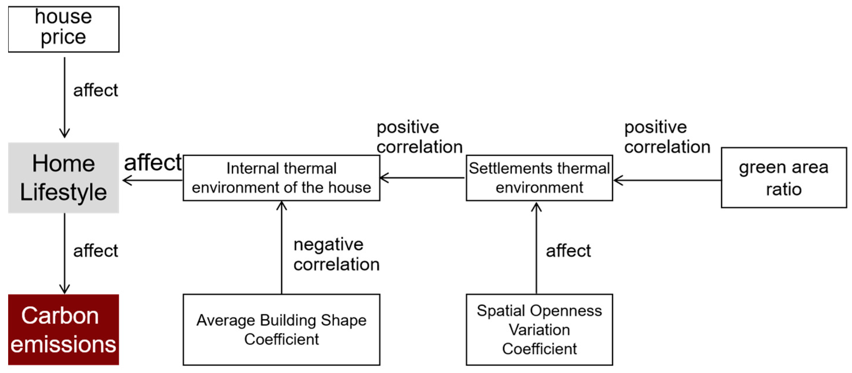
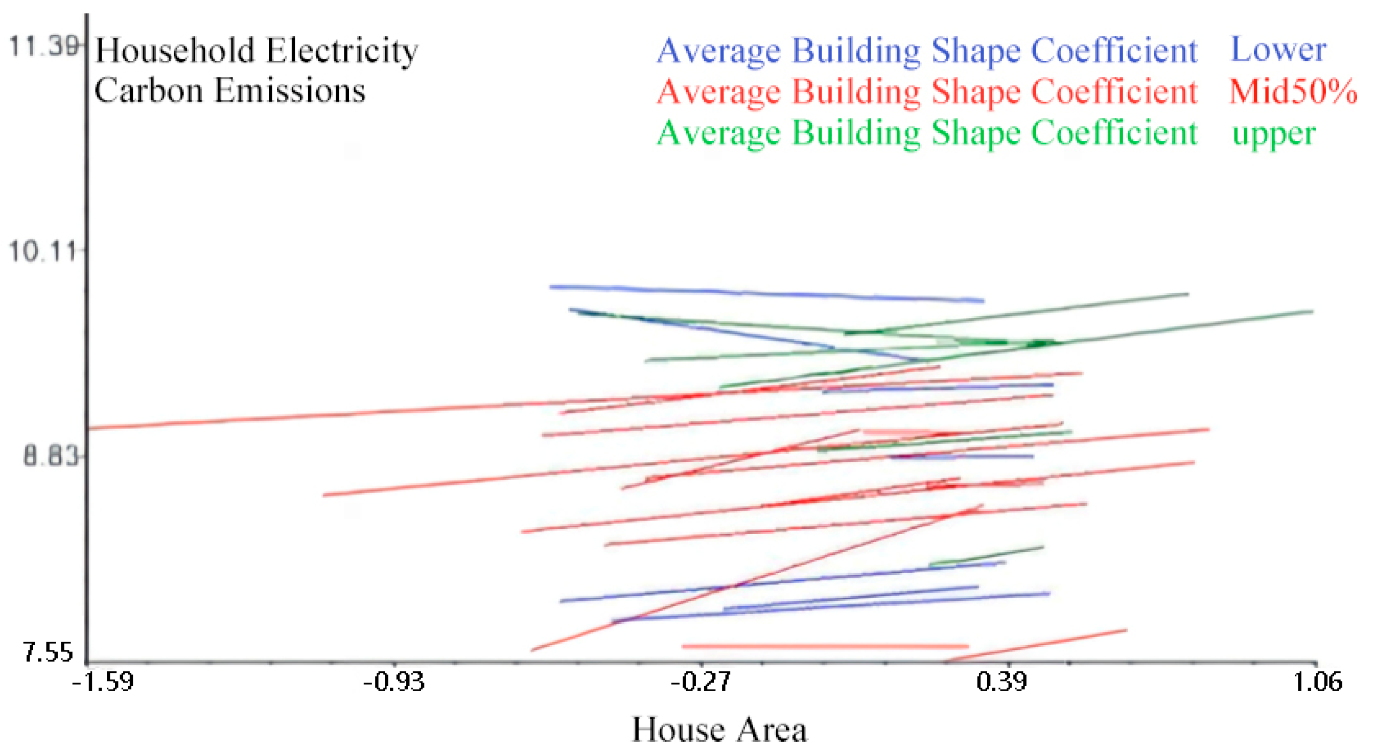
The average building shape coefficient is the most critical spatial morphological indicator. Higher coefficients—representing larger envelope surface area relative to building volume—increase heat exchange and cooling demand, thereby raising household electricity carbon emissions. Beyond its direct effect, the HLM results reveal a significant cross-level interaction between the average building shape coefficient (residential area level) and housing area (dwelling level). Specifically, as the average building shape coefficient increases, the positive relationship between housing area and electricity-related carbon emissions becomes stronger. In other words, larger dwellings lead to a disproportionately higher increase in electricity emissions when they are located in residential area characterized by more complex or less compact building forms.

This moderating effect is illustrated in Figure 9, where the slope of housing area steepens under higher levels of the building shape coefficient, indicating an amplification of dwelling-size effects by unfavorable building morphology. Such direct statistical evidence underscores the importance of building shape control as a planning and design lever, particularly for envelope optimization and dwelling layout strategies in high-density residential area.

Residential land area shows a positive association with electricity emissions. Larger developments, typically farther from urban centers with larger dwellings and distinct demographics, indirectly increase energy consumption. This effect is moderately supported by HLM, indicating that land allocation and development intensity should be considered in spatial planning.

Other indicators, such as spatial openness variation and green space ratio, show weaker or less stable effects in the HLM results. Their influence is primarily indirect, mediated by microclimatic conditions (shading, ventilation, heat dissipation). Although the statistical support is limited, these factors remain relevant for planning guidance based on prior literature and environmental logic, suggesting potential benefits from optimizing green space distribution and open area configuration.

By distinguishing strongly supported factors (building shape coefficient, housing area, land area) from speculative or context-dependent factors (green space ratio, spatial openness), planners can prioritize interventions with empirical backing while considering complementary measures informed by environmental principles (Figure 10).

4.3.4. Influencing Factors and Mechanisms at the Dwelling Scale

According to the full HLM results, dwelling-scale factors play a dominant role in explaining household electricity carbon emissions. Variables such as air-conditioning usage duration, housing area, building orientation, and building type exhibit relatively stronger associations, all showing positive relationships with electricity-related carbon emissions. Among these, housing area and building orientation represent the most relevant spatial morphological characteristics at the dwelling scale.

Larger dwellings tend to accommodate more residents and electrical equipment, resulting in higher electricity demand and associated carbon emissions (Figure 11). Building orientation primarily affects household electricity carbon emissions through its influence on indoor thermal and lighting conditions. Previous studies [31] have shown that south-facing dwellings benefit from improved natural lighting and reduced lighting demand, while west-facing dwellings are subject to greater solar heat gain in summer, increasing cooling energy consumption.

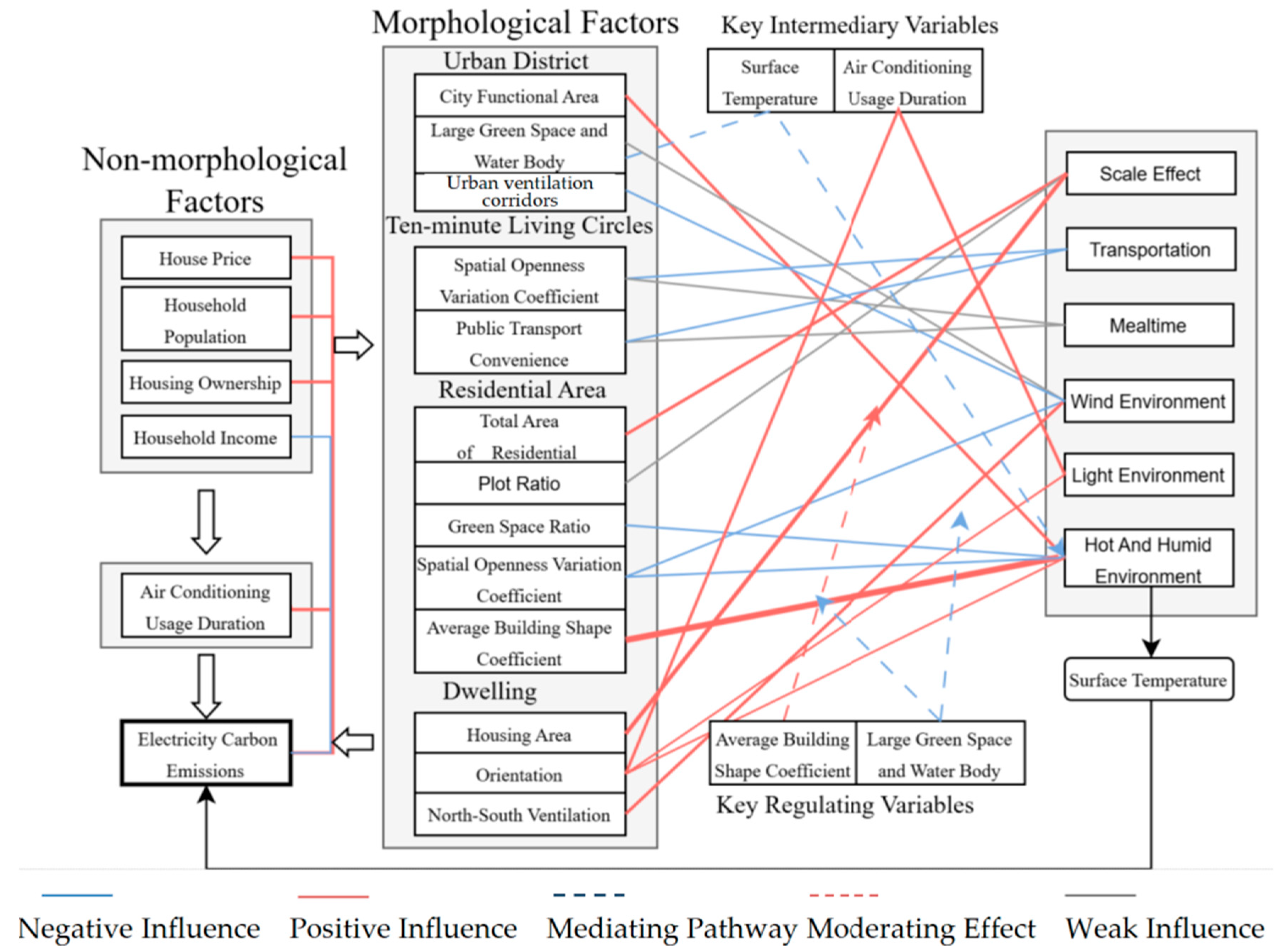
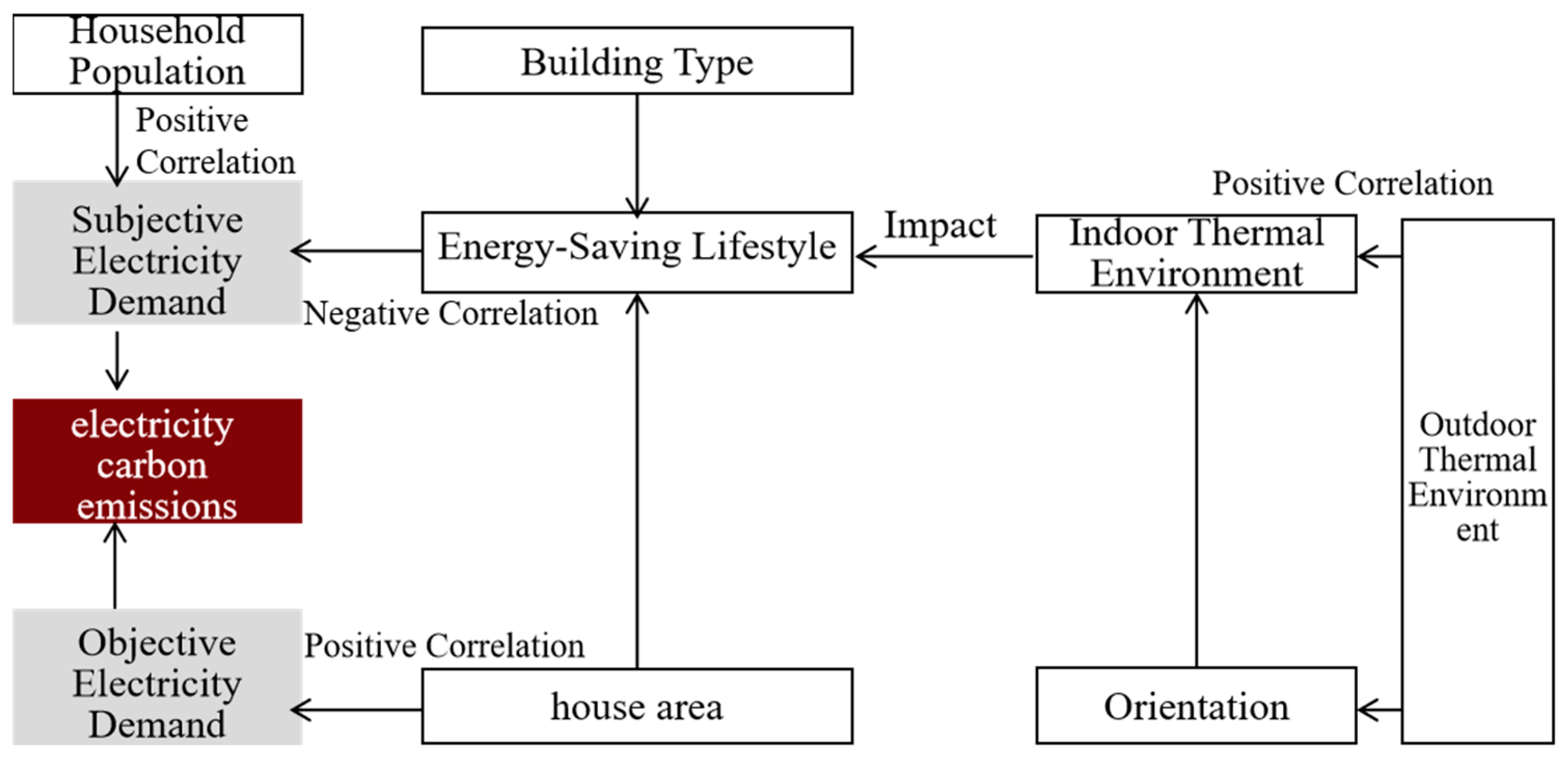
Synthesizing the influence pathways of key spatial morphological factors across scales, two principal mechanisms can be identified. First, scale-related indicators—such as residential land area, building area, and floor area ratio—affect household electricity carbon emissions by shaping development intensity, building size, and thermal environments. Excessive development intensity and high floor area ratios in high-density urban contexts can exacerbate heat accumulation and cooling demand, thereby increasing electricity-related emissions. Second, microclimatic modulation plays a mediating role, whereby green spaces, water bodies, and building layout influence local wind, shading, and thermal conditions, ultimately affecting household electricity use behavior.

Based on these findings, an integrated influence mechanism model of household electricity carbon emissions in urban residential area is proposed (Figure 12), providing a conceptual framework to support carbon-reduction strategies at multiple spatial scales.

5. Conclusions and Discussion

Residential area is major sources of urban carbon emissions, particularly in high-density cities where population concentration, compact built form, and intensive energy use coincide. Once established, residential spatial morphology can generate a long-term lock-in effect on household electricity-related emissions, thereby constraining the effectiveness of short-term behavioral or technological interventions.

Using a multilevel framework that integrates dwelling, residential area, Ten-Minute Living Circles, and urban district scales, and applying hierarchical linear modelling (HLM), this study finds that household electricity carbon emissions are primarily driven by dwelling-level characteristics, while residential area morphology plays a substantial contextual role. Urban-district factors mainly operate indirectly through climatic and functional conditions, whereas Ten-Minute-Living-Circle indicators show limited direct effects in the final HLM.

The influence of spatial form is scale-dependent and mediated by cross-level interactions. Core indicators, including housing area, building orientation, and the average building shape coefficient, affect emissions not only through direct associations but also by conditioning household-level energy demand. For example, the positive relationship between dwelling size and electricity-related carbon emissions becomes stronger in residential areas with higher average building shape coefficients, highlighting the moderating role of building morphology.

From a planning perspective, the final HLM identifies a small set of levers with the most consistent and statistically robust effects. Housing area, average building shape coefficient, and residential land area can be classified as model-derived factors because they exhibit statistically significant and stable effects in the full multilevel specification. These variables therefore represent the most robust spatial determinants of household electricity carbon emissions in this study and can be translated into relatively rigid, upstream low-carbon planning measures. By contrast, Large Green–Blue Space and district-scale ventilation corridors are better characterized as model-informed measures, whose influences are mainly indirect or context-dependent and can be applied as more flexible guiding strategies. This distinction clarifies the relative empirical strength of different planning-related factors and improves the transparency of result interpretation (

Table 11. Overview table of key spatial morphological factors influencing household electricity carbon emissions.

Influencing Factor	Influence Effect	Relative Importance (Within Scale)	Planning Rules	Evidence Basis
Urban District–level factors mainly exert indirect and contextual influences on household electricity carbon emissions.
City functional area	Ecological belt < General < Tech/industrial < Core	1	Avoid locating high-density housing in high-heat functional cores; prioritize ecological or mixed zones.	Model-informed + literature-supported
Urban ventilation corridors	Negative correlation, direct influence effect not significant	2	Preserve ventilation corridors as district-scale climatic infrastructure.	Model-informed + literature-supported
Large green–blue spaces	Negative correlation, direct influence effect not significant	3	Large Green–Blue Spaces mitigates orientation-related cooling demand by moderating surface temperature; benefits are context-dependent and strongest at larger spatial extents.	Model-informed (moderated effect)
The effect of Ten-Minute Living Circles is not significant
Spatial openness variation coefficient	Direct influence effect not significant	/	Limited direct association with household electricity emissions, suggesting its primary relevance lies in transport-related carbon emissions rather than residential electricity use.
Public transport convenience		/
Residential-area-level factors play a substantial contextual role by shaping building morphology and microclimatic conditions.
Average building shape coefficient	Positive correlation	1	Most critical residential area-scale morphological factor; compact building forms with lower shape coefficients should be prioritized to reduce envelope-driven cooling demand, especially for large dwellings.	Model-derived (significant coefficient + cross-level interaction)
Total residential land area	Positive correlation	2	Excessively large residential land parcels in high-density contexts are associated with higher household electricity emissions; moderate land scale is preferable for energy efficiency.	Model-derived (significant coefficient)
Green space ratio	Negative correlation	3	Cooling benefits exist but are constrained by low tree coverage and fragmentation; effectiveness depends on vegetation quality rather than percentage alone.	Model-informed + literature-supported
Spatial openness variation coefficient	Negative (direct effect not significant)	4	microclimatic effects suggest diminishing marginal returns of openness in already dense residential area.	Model-informed + literature-supported
Floor area ratio	Direct influence effect not significant	/	The floor area ratio and building density indicators in high-density residential area have a relatively weak impact on household electricity carbon emissions.
Building density	Direct influence effect not significant	/
Dwelling-scale factors exert the strongest and most direct influence on household electricity carbon emissions.
Housing area	Positive correlation	1	Most influential dwelling-scale factor; controlling excessive dwelling size is critical, particularly in communities with high building shape coefficients.	Model-derived (largest standardized coefficient)
North–south ventilation	Negative correlation	2	Effective ventilation reduces cooling demand; benefits are amplified in high-quality residential environments.	Model-derived
Building orientation	Positive correlation	3	North–south orientation is associated with lower electricity-related carbon emissions, but its effectiveness is conditioned by surrounding Large Green–Blue Spaces and microclimate.	Model-informed (moderated effect)

).

Limitations include the focus on a single Beijing district, restriction to “standard families,” use of fixed emission factors, and potential post-pandemic survey biases. Future research should expand geographic coverage, include diverse household types, and incorporate dynamic energy and behavioral data to refine multiscale carbon emission assessments.