Comparative Study on Model Applicability for Longitudinal Seismic Response of Shield Tunnels Under Design Earthquake Loading

Abstract

To investigate model applicability for the seismic analysis of shield tunnels in adverse geological sections, this study compares the beam–spring model (BSM) and mass–beam–spring model (MBSM). The Shantou Bay subsea shield tunnel, located in a Seismic Fortification Intensity Degree 8 region (PGA = 0.15 g), is used as the case study. Based on the Response Displacement Method, numerical simulations were conducted via ABAQUS and Python (Version 2.7) scripts to evaluate dynamic responses under unidirectional and tri-directional ground motions. Results indicate that while both models capture longitudinal response patterns, significant amplitude differences exist. Specifically, by accounting for soil inertial effects and shear transfer, the MBSM yields peak relative displacements, joint openings, and internal forces at soft–hard rock interfaces that are approximately 60–130% higher than those of the BSM. Furthermore, tri-directional input significantly amplifies structural responses, exhibiting distinct abrupt changes at geological transition zones. These findings provide a vital reference for the seismic design of shield tunnels traversing complex geological conditions.

1. Introduction

With the rapid expansion of urban rail transit networks and cross-sea infrastructure in China, an increasing number of long-distance shield tunnels are being constructed through complex geological environments, particularly in soft soil regions like the Greater Bay Area. These tunnels inevitably traverse adverse geological sections, such as active fault zones, liquefiable soil layers, and sharp interfaces between soft and hard strata [1,2]. Under the coupling effect of non-uniform seismic excitation and adverse geological conditions, abrupt changes in surrounding rock stiffness induce significant differential forced displacements in the tunnel structure. Consequently, this triggers a series of seismic resilience challenges, including uneven distribution of internal forces, excessive opening of segment joints, and localized longitudinal deformation, which pose severe threats to the operational safety of the lifecycle infrastructure.

Field investigations from historical strong earthquakes have repeatedly confirmed that adverse geological zones constitute the most vulnerable links in the seismic performance of underground structures. While early events demonstrated the general risk of fault crossing, recent seismic events have provided fresh and detailed evidence of this vulnerability. For instance, the 2008 Wenchuan earthquake induced severe vault collapse and shear dislocation in the Longxi Tunnel, which was directly attributed to fault rupture [3]. More recently, the 2022 Menyuan earthquake (Ms 6.9) in Qinghai Province caused a drastic misalignment of 2.7 m and an S-shaped rail deformation in the Daliang Tunnel of the Lanzhou–Xinjiang High-Speed Railway [4,5]. Furthermore, damage surveys from the 2023 Turkey–Syria earthquake sequence highlighted that tunnels and underground lifelines in soft alluvial deposits or fault zones experienced significantly higher damage levels compared to those in stable rock, primarily due to kinematic interaction effects [6]. These severe dislocation and deformation phenomena exhibit pronounced local inertial effects, suggesting that traditional static or quasi-static simplified models possess inherent limitations in predicting such non-uniform ground responses.

Currently, seismic analysis methods for tunnels are categorized into numerical simulation methods and simplified analytical models [7]. The Two-Dimensional Finite Element Method (2D FEM) is commonly employed for transverse seismic analysis. The Three-Dimensional Finite Element Method (3D FEM) is theoretically rigorous and capable of capturing complex boundary conditions and nonlinear soil–structure interaction (SSI) [8,9]. However, for long-distance tunnels extending several kilometers, the immense computational cost and modeling complexity of 3D FEM hinder its extensive application in parametric design and rapid assessment, as highlighted in recent studies [10]. Consequently, efficient simplified models based on the Response Displacement Method (RDM) remain the prevailing strategy in engineering practice. The beam–spring model (BSM), typically implemented within the RDM framework, where Miao et al. [11] demonstrated its feasibility in practical engineering analysis, simplifies tunnel segments into beam elements and utilizes ground springs to simulate SSI. This model is widely adopted in design codes and academic research for various underground line structures, including shield tunnels and buried pipelines [12]. Recent studies have further extended the BSM to analyze complex joint behaviors, such as flexible joints with longitudinal limit devices [13]. However, despite its versatility, the BSM inherently neglects the inertial forces of the structure and the surrounding soil mass. This simplification is generally acceptable for uniform stiff sites but may underestimate the structural response in soft soil regions where dynamic amplification is dominant.

To overcome the limitations of the quasi-static BSM, the mass–beam–spring model (MBSM) and related refined modeling techniques have gained increasing attention. By discretizing the surrounding soil into equivalent mass points connected to the structure via springs, these models effectively account for both kinematic interaction and inertial effects. Yu et al. [14], Wu et al. [15], and Yu-an et al. [16] pioneered the application of this model in the seismic response analysis of immersed tunnels, verifying its calculation accuracy and applicability. Recent studies have further validated the efficacy of the multiple mass–beam–spring model in capturing the dynamic response of immersed tunnels equipped with specialized joint devices [17] and in optimizing backfilling schemes [18]. Given the structural similarities in longitudinal behavior between immersed and shield tunnels, this method has subsequently been extended to the seismic research of cross-sea shield tunnels. Furthermore, based on the multi-mass–beam–spring model, Yu et al. [14] proposed a longitudinal multi-scale coupled seismic analysis method for long-distance shield tunnels, aiming to strike a balance between the accuracy of refined joint simulations and computational efficiency. Recent advancements have further extended these concepts to investigate the soil–tunnel interaction under complex longitudinal seismic excitations [19] and to develop refined models for specific damage assessment [20]. Despite these theoretical advancements in seismic response analysis [21], a systematic comparative study of the BSM and MBSM under identical engineering contexts—specifically regarding their discrepancy patterns in soft–hard geological transitions—remains limited. To address the aforementioned limitations, this study relies on the engineering background of the Shantou Bay subsea shield tunnel to establish both the beam–spring model and the mass–beam–spring model for a comparative analysis of longitudinal seismic responses. The study investigates the discrepancy patterns in key response indices—including structural internal forces, segment joint openings, and relative displacements—under various seismic inputs and geological conditions. The specific objectives are to (1) clarify the response discrepancies and applicable boundaries of the two models; (2) propose recommendations for model selection and parameter configuration suitable for long-distance shield tunnels; and (3) provide theoretical and engineering references for the seismic design of shield tunnels traversing adverse geological sections.

2. Model Description and Analysis Method

2.1. Longitudinal Beam–Spring Model

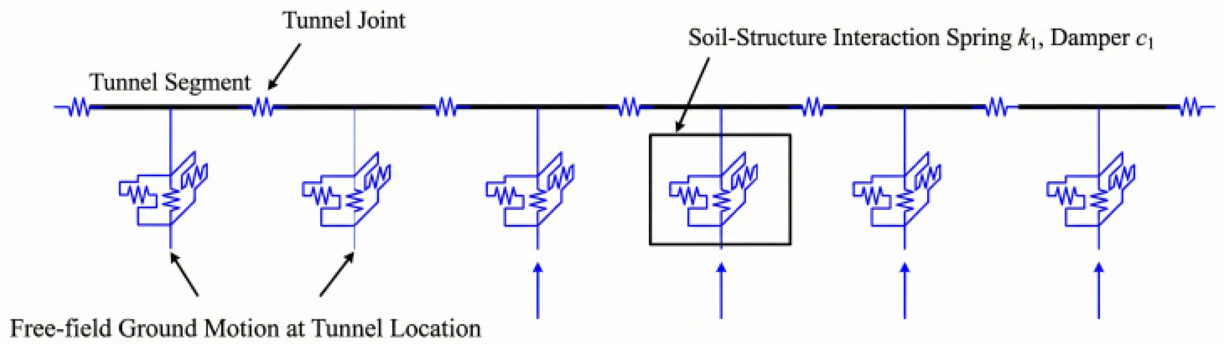
The longitudinal beam–spring model is an equivalent continuous model established based on the Timoshenko beam theory. Unlike the Euler–Bernoulli beam theory, the Timoshenko theory explicitly accounts for transverse shear deformation, which is non-negligible for large-diameter shield tunnel structures. In this model, shield tunnel segments are simplified as beam elements with equivalent cross-sectional properties. To simulate the confinement of surrounding rock and soil–structure interaction under seismic loading, ground springs are arranged at each beam node. One end of the spring is connected to the tunnel beam node, while the other end serves as the excitation input point for imposing the seismic displacement time histories calculated from the free field (as shown in Figure 1). Furthermore, the connection stiffness between tunnel segments is simulated using nonlinear springs, where the mechanical characteristics of bolts and joints are reflected by defining axial tension–compression stiffness and rotational stiffness.

Parameters of Soil–Structure Interaction Springs

In the beam–spring model, the stiffness parameters of the ground springs are critical determinants of simulation reliability, and their values depend on the physical and mechanical properties of the soil layers at the tunnel site. Based on the Code for Seismic Design of Buildings (GB50011-2010) [22] and relevant industry standards, this study adopts the coefficient of subgrade reaction method to determine the stiffness of the soil–structure interaction springs.

Assuming the foundation soil is a homogeneous and isotropic medium, the stiffness of the springs surrounding the tunnel structure can be calculated using the coefficient of subgrade reaction. The formulas are as follows:

$$K_t = K·L·W$$

(1)

$$K_1=1/3K_t$$

(2)

where $K_t$ represents the transverse (or normal) ground spring stiffness (N/m); $K_1$ represents the longitudinal ground spring stiffness (N/m), which is typically taken as 1/3 of the transverse stiffness; K denotes the coefficient of subgrade reaction ($\mathrm{N}/{\mathrm{m}}^3$), reflecting the soil’s resistance to deformation; L is the spacing between adjacent ground springs in the model (m), taken as 1.0 m in this study; W represents the tunnel diameter (m).

2.2. Mass–Beam–Spring Model

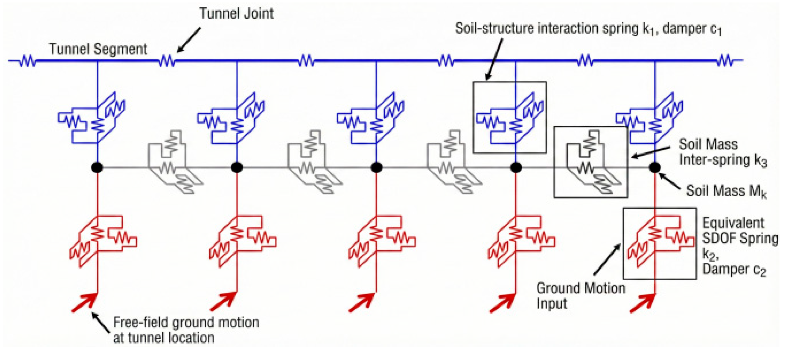
To account for the significant inertial effects and ground non-uniformity associated with long-distance tunnels under seismic action, the mass–beam–spring model is established. Based on the Timoshenko beam theory, this model simulates tunnel segments as beam elements. Simultaneously, the surrounding rock is discretized longitudinally according to the segment width. Each soil slice unit is simplified into a single mass point with equivalent mass, which is connected to the beam element via springs and dampers, thereby constituting a multi-mass dynamic system. The schematic configuration of the model is shown in Figure 2. The key components of the model are defined as follows:

The mass of each soil point ($M_k$) is determined by the first-mode effective mass of the corresponding soil slice unit. The soil–structure interaction springs ($K_1$) and dampers ($C_1$) are employed to simulate the dynamic coupling between the surrounding rock and the tunnel segments. The equivalent input springs ($K_2$) and dampers ($C_2$) connect the soil mass points to the dynamic input nodes to transmit seismic loads. The inter-mass springs between soil points ($K_3$) are utilized to simulate the transmission of shear deformation and inertial coupling effects within the soil.

Determination of Model Parameters

In the mass–beam–spring model, the mass of the soil points and the stiffness parameters of the associated springs are primarily determined by the shear wave velocity and density of the site soil layers. Based on the principle of one-dimensional ground response analysis and the research findings of Yu et al. [14], the specific calculation procedure for these parameters is as follows:

(1)

Equivalent Mass of Soil Point $M_k$

The mass $M_k$ assigned to the k-th soil slice does not represent the total physical mass of the soil; rather, it corresponds to the effective mass derived from the first-order shear mode. First, the first-mode effective mass per unit length, denoted as $M_e$, is calculated using Equation (3). Subsequently, the mass of the discrete point is determined via Equation (4):

$$M_e = {\displaystyle \frac{{\left({\sum }_{i=1}^n{m}_i{\varphi }_i\right)}^2}{{\sum }_{i=1}^n{m}_i{\varphi }_i^2}}$$

(3)

$$M_k=M_e·L_k$$

(4)

where $m_i$ represents the mass of the i-th soil layer, determined by the soil density $\rho$; ${\varphi }_i$ denotes the first-order mode shape vector (or coefficient) of the i-th soil layer; n is the total number of soil layers; $L_k$ represents the thickness of the k-th soil slice.

(2)

Stiffness of Connecting Springs between Adjacent Mass Points ($K_2$)

To simulate the longitudinal continuity of the soil along the tunnel, longitudinal tension–compression springs ($K_{2x}$) and shear springs ($K_{2y},K_{2z}$) are arranged between adjacent mass points. The stiffness of these springs is determined by the shear modulus $G_i$ (where $G_i$ = $\rho {\mathrm{V}}_{\mathrm{s}}^2$) of the adjacent soil slices and their cross-sectional parameters:

$$K_{2x}= {\displaystyle \frac{1}{L_k}}\sum _{i=1}^n{E}_i{A}_i{\delta }_i$$

(5)

$$K_{2y}=K_{2z}={\displaystyle \frac{1}{L_k}}\sum _{i=1}^n{G}_i{A}_i{\delta }_i$$

(6)

(3)

Stiffness of Equivalent Soil Springs ($K_3$)

The parameter $K_3$ reflects the self-vibration characteristics of a single soil slice unit under bedrock excitation. Based on the first-order natural circular frequency ${\omega }_k$ of the soil, the horizontal ($K_{3x}{,K}_{3y}$) and vertical ($K_{3z}$) stiffnesses are calculated as follows:

$$K_{3x} = K_{3y} = M_k·{\omega }_k^2$$

(7)

$$K_{3z}=K_{3x}·{\displaystyle \frac{2(1+\nu )}{1-2\nu }}$$

(8)

where ${\omega }_k=2\mathsf{\pi }/{\mathrm{T}}_{\mathrm{k}}$ represents the first-order natural circular frequency of the soil slice, which is determined by the soil layer thickness and the shear wave velocity $V_s$; $\nu$ denotes Poisson’s ratio of the soil.

(4)

Damping Coefficient $C_3$

To account for the energy dissipation characteristics of the soil, corresponding dampers $C_3$ are incorporated into the model. The damping coefficients are calculated based on the first-order natural frequency of the soil slice unit, utilizing the following formula:

$$C_{3x} = C_{3y} = 2\beta M_k·{\omega }_k$$

(9)

$$C_{3z}=C_{3x}·\sqrt{{\displaystyle \frac{2(1-\nu )}{1-2\nu }}}$$

(10)

where $\beta$ denotes the damping ratio, which is taken as 0.05.

In this simplified discrete model, the radiation damping effect at the truncated boundaries is not explicitly modeled using absorbing boundary elements. Instead, it is approximated by the equivalent viscous dampers ($C_1$, $C_3$) incorporated into the system.

2.3. Longitudinal Equivalent Stiffness Model of Tunnel Segments

The mechanical behavior of shield tunnel segments under longitudinal seismic action is jointly governed by the bending stiffness of the segments themselves and the mechanical properties of the connecting joints between adjacent rings. Based on the equivalent continuous model and existing research [23], the longitudinal connections between tunnel rings are simulated using tension–compression asymmetric springs and rotational springs. Furthermore, the mechanical characteristics of the connecting bolts are simulated by defining nonlinear load–deformation curves.

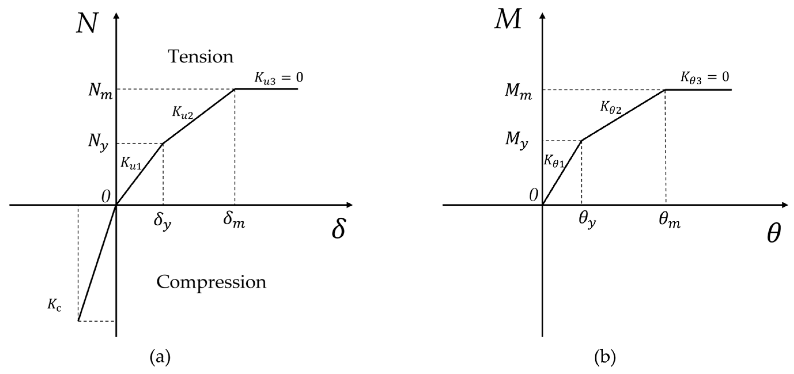
The inter-ring joints exhibit significant nonlinearity and tension–compression asymmetry. Under tension, the load is primarily borne by the connecting bolts; under compression, the load is borne by the concrete contact surfaces of the segments. When adjacent rings undergo bending deformation, the internal forces in the tensile and compressive zones are borne independently by the bolts and the concrete, respectively. The constitutive relations for the tension–compression asymmetric springs and the nonlinear rotational springs are illustrated in Figure 3a,b.

3. Project Overview and Model Parameters

3.1. Project Overview and Model Parameters

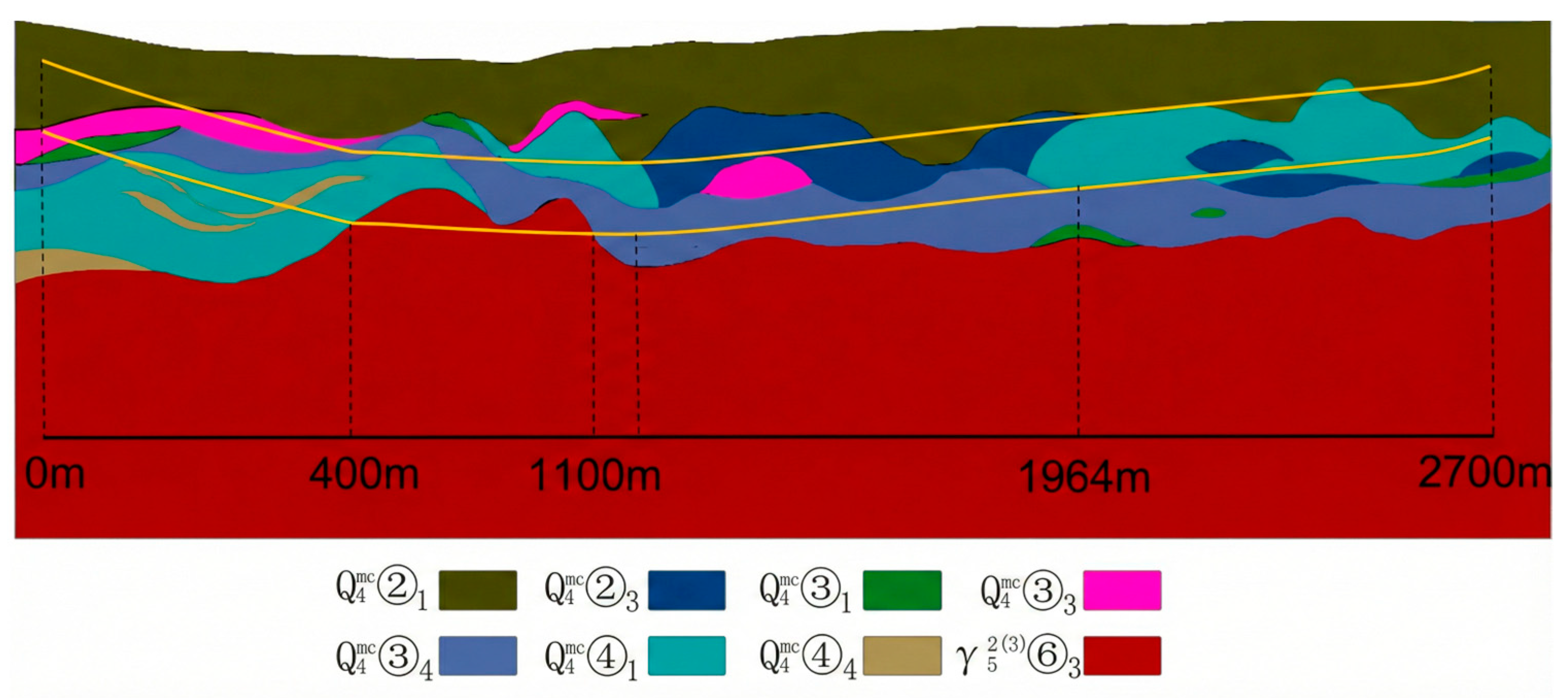
The Shantou Bay subsea shield tunnel, the first super-large diameter shield tunnel in China, is located in a seismic intensity zone VIII area and traverses complex subsea geology, presenting significant technical challenges. The outer and inner radii of the tunnel segments are 7.25 m and 6.65 m, respectively. In this study, a beam element model is established in ABAQUS based on the Timoshenko beam theory. The finite element mesh size is set to 1.0 m, and the entire tunnel is discretized into 1350 beam elements. The distribution of soil layers and the location of the tunnel are shown in Figure 4. The parameters of the soil layers are listed in

Table 1. Physical and mechanical parameters of soil layers.

Soil Classification	Density (kg/m3)	Poisson’s Ratio	Elastic Modulus (MPa)	Shear Wave Velocity (m/s)
${\mathrm{Q}}_4^{\mathrm{m}\mathrm{c}}{\mathrm{②}}_1$ Muck	15.5	0.45	2	121
${\mathrm{Q}}_4^{\mathrm{m}\mathrm{c}}{\mathrm{②}}_3$ Sandy Muck	18.5	0.35	4	162
${\mathrm{Q}}_4^{\mathrm{m}\mathrm{c}}{\mathrm{③}}_1$ Silty Clay	20.0	0.30	15	230
${\mathrm{Q}}_4^{\mathrm{m}\mathrm{c}}{\mathrm{③}}_3$ Mucky soil	18.5	0.3	10	121
${\mathrm{Q}}_4^{\mathrm{m}\mathrm{c}}{\mathrm{③}}_4$ Medium Coarse Sand	20.0	0.25	20	268
${\mathrm{Q}}_4^{\mathrm{m}\mathrm{c}}{\mathrm{④}}_1$ Mucky soil	17.0	0.25	4	121
${\mathrm{Q}}_4^{\mathrm{m}\mathrm{c}}{\mathrm{④}}_4$ Medium Coarse Sand	20.0	0.25	10	268
${\mathsf{\gamma }}_5^{2\left(3\right)}{\mathrm{⑥}}_3$ Granite	26.7	0.25	106,000	868

.

The tunnel site exhibits complex geological conditions characterized by significant spatial variability. As illustrated in Figure 4, the tunnel traverses multiple distinct strata, including thick layers of mucky soil (soft soil), silty clay, medium-coarse sand, and protruding granite bedrock (hard rock). Table 1 lists the detailed physical and mechanical parameters of these soil layers. Notably, the tunnel passes through several abrupt geological transition zones (e.g., at mileage 600 m and 1100 m), where the surrounding medium changes sharply from soft mucky soil to hard granite. These sections represent typical ‘adverse geological conditions’, where the contrast in stiffness and mass induces significant differential seismic ground motion.

The coefficient of subgrade reaction for the foundation soil is determined in accordance with the current national standard Code for Seismic Design of Nuclear Power Plants (GB 50267). Combined with the specific engineering geological conditions, the parameters for the soil–structure interaction springs at the tunnel crown, side, and bottom are listed in

Table 2. Spring parameters at the tunnel crown.

Section (m)	0–400	400–600	600–1100	1100–1964	1964–2700
Spring stiffness (GN/m)	6.41	0.09	6.41	0.15	0.11

,

Table 3. Spring parameters at the tunnel side.

Section (m)	0–400	400–600	600–1100	1100–1950	1950–2158	2158–2323	2323–2700
Spring stiffness (GN/m)	6.41	0.09	6.41	0.15	0.11	0.15	0.11

and

Table 4. Spring parameters at the tunnel bottom.

Section (m)	0–600	600–1100	1100–1160	1160–1964	1964–2700
Spring stiffness (GN/m)	0.11	41.78	0.29	6.41	0.11

. All spring stiffnesses and damping coefficients are derived from the physical and mechanical parameters of the soil layers. The specific spring parameters and damping coefficients for the mass–beam–spring model are presented in

Table 5. Spring stiffness and damping coefficients of the mass–beam–spring model.

Soil–Structure Interaction Springs						Inter-Mass–Spring Stiffness /(108 N·m−1)		Equivalent Mass–Spring				Mass of Soil Point /(107 kg)
Section	Spring Stiffness /(108 N·m−1)			Damping Coefficients /(108 N·s·m−1)				Spring Stiffness /(108 N·m−1)		Damping Coefficients /(108 N·s·m−1)
	${\mathit{K}}_{1\mathit{x}}$	${\mathit{K}}_{1\mathit{y}}$	${\mathit{K}}_{1\mathit{z}}$	${\mathit{C}}_{1\mathit{x}}$	${\mathit{C}}_{1\mathit{x}},{\mathit{C}}_{1\mathit{z}}$	${\mathit{K}}_{2\mathit{x}}$	${\mathit{K}}_{2\mathit{y}},{\mathit{K}}_{2\mathit{z}}$	${\mathit{K}}_{3\mathit{x}},{\mathit{K}}_{3\mathit{y}}$	${\mathit{K}}_{3\mathit{z}}$	${\mathit{C}}_{3\mathit{x}},{\mathit{C}}_{3\mathit{y}}$	${\mathit{C}}_{3\mathit{Z}}$	m
1	2.13	20.5	0.9	1.21	0.482	1.21	0.482	1.55	2.16	5.46	8.7	1.92
2	1.32	4.11	2.99	1.51	0.0702	1.51	0.0702	1.95	1.23	6.24	8.11	2.01
3	3.35	7.82	2.07	2.23	0.996	2.23	0.996	2.55	2.12	7.56	10.8	2.57
4	6.58	1.78	6.01	2.01	1.070	2.01	1.070	2.59	1.99	6.84	9.82	2.38
5	2.02	3.52	2.74	1.41	0.590	1.41	0.590	1.93	1.38	5.41	7.54	1.80
6	3.82	3.26	3.74	1.94	1.03	1.94	1.03	3.41	1.26	6.83	9.64	1.59

.

3.2. Selection and Input of Ground Motions

According to the Code for Seismic Design of Urban Rail Transit Structures (GB 50909-2014) [24], the tunnel site is classified as a Type III site (soft soil) within a region of Seismic Fortification Intensity Degree 8. Consequently, the input ground motions are selected and scaled to match the Design Basis Earthquake (DBE) level, with a Peak Ground Acceleration (PGA) of 0.15 g (150 Gal).

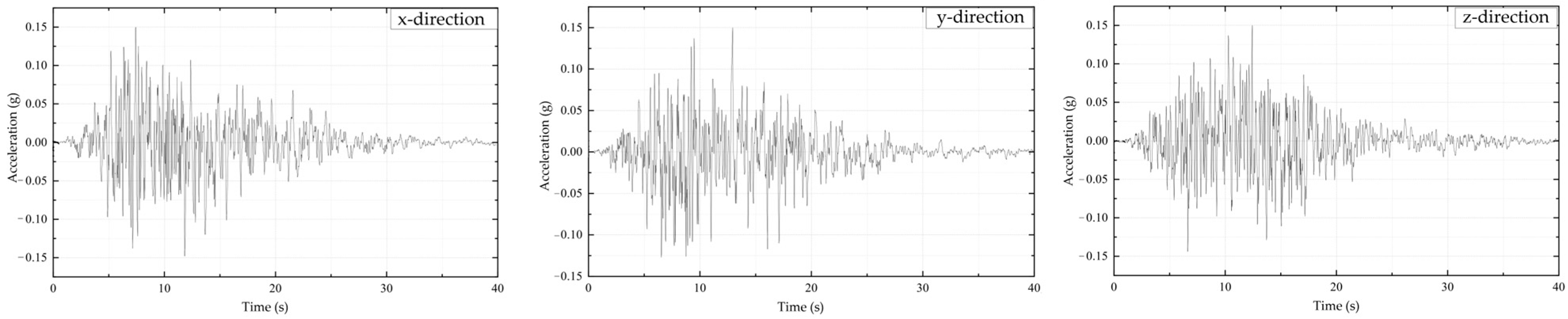
The standard response spectrum of the site surface, determined by the Seismic Performance Research Report of the Su-Ai Passage issued by the Earthquake Administration, was selected as the target spectrum [25]. Artificial seismic waves were synthesized using the Abrahamson–Hancock wavelet algorithm [26], which is based on the relationship between power spectra and acceleration response spectra. During the synthesis process, the spectral period range was controlled between 0.04 s and 7.0 s, and the relative iteration error between the fitted spectrum and the target spectrum was strictly limited to within 5%. The acceleration time histories of the synthesized waves are shown in Figure 5.

The input methods for the ground motions differ between the two models: (1) For the mass–beam–spring model, the artificial acceleration time histories were directly input at the base (or distal end) of the equivalent soil–spring system. (2) For the beam–spring model, based on the Response Displacement Method, the same artificial waves were first input into a free-field model. The seismic displacement time histories at the depth of the tunnel axis were obtained via dynamic analysis and subsequently applied as forced displacement boundaries at the external input nodes of the ground springs.

In the beam–spring model (BSM), the longitudinal seismic response is primarily governed by the relative deformation of the surrounding ground. To accurately capture the nonlinear behavior of the soft soil under seismic excitation, a 1D free-field site response analysis was strictly conducted prior to the BSM calculation. This analysis utilized the equivalent linearization method to generate the displacement time histories at different depths. Consequently, although the soil–structure interaction springs in the BSM were simplified as linear elastic elements to facilitate comparison, the input displacement field applied to the springs already inherently reflects the stiffness degradation and hysteresis characteristics of the soil.

The free-field site response analysis was performed using the specific code. This program was selected for its efficiency in implementing the equivalent linearization method in the frequency domain.

The ground motions were applied under two loading conditions: longitudinal unidirectional input and tri-directional input. By comparing the internal forces of the tunnel segments, peak relative displacements, and maximum segment joint openings, the response differences between the two models under identical conditions were analyzed.

4. Comparison of Calculation Results

4.1. Comparison of Internal Forces in Shield Tunnel

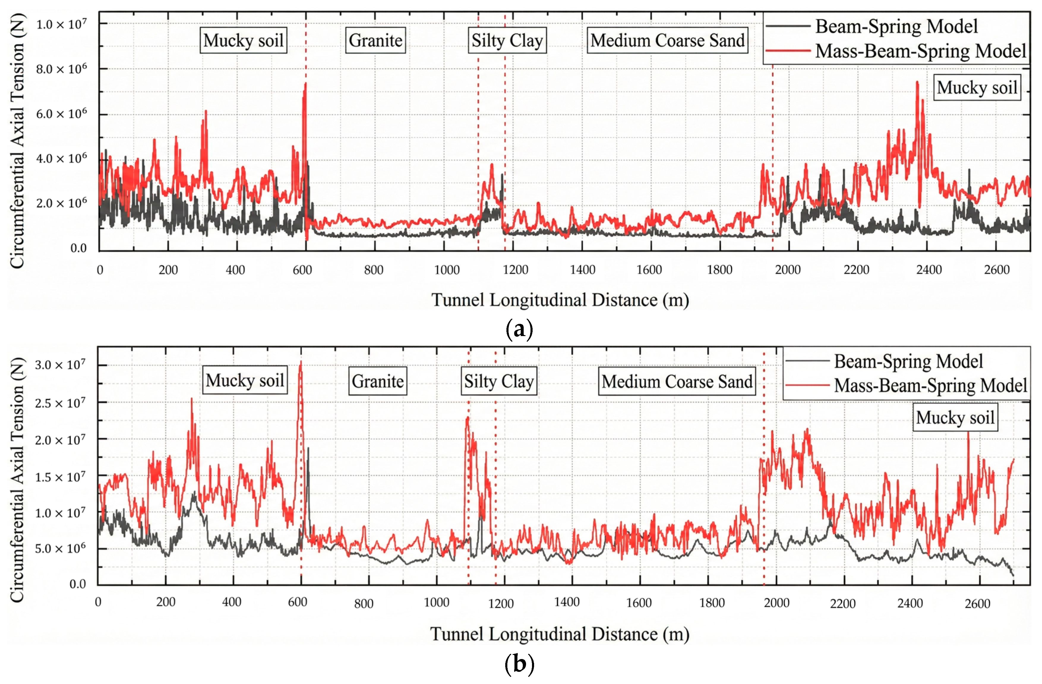
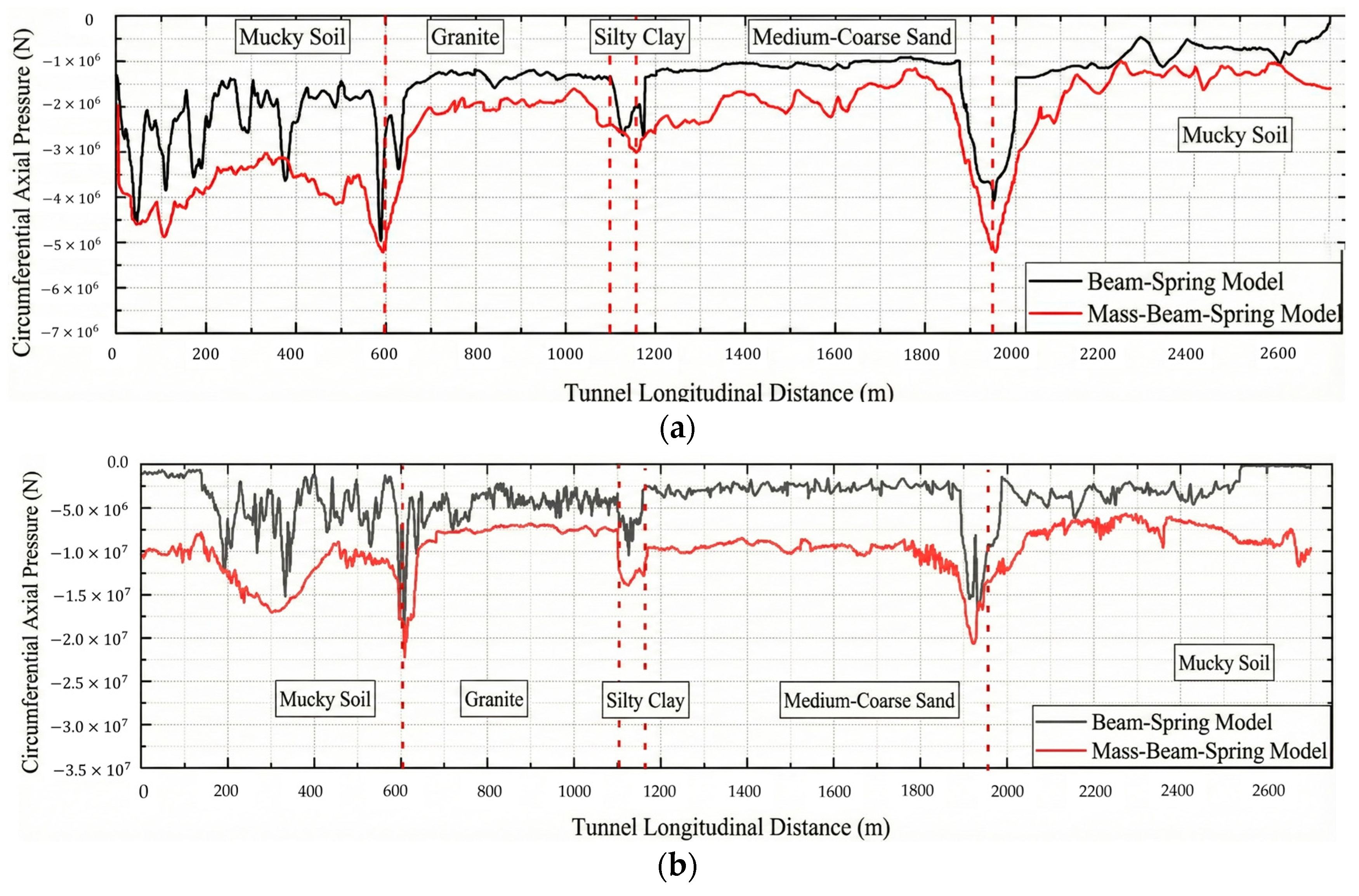
Upon completion of the numerical simulations, the internal force responses of all tunnel segments across all analysis steps were extracted for both models, and the peak values were identified. Maximum internal force envelope diagrams were plotted against the longitudinal tunnel length, as shown in Figure 6 and Figure 7. In these figures, the black curves represent the results obtained from the beam–spring model, while the red curves denote the results from the mass–beam–spring model.

Both models exhibit significant peaks at the interface zones where surrounding rock properties undergo abrupt changes. Specifically, these locations include the 600 m mark (mucky soil/granite interface), the 1100 m mark (granite/silty clay interface), and the 1964 m mark (medium-coarse sand/mucky soil interface). Conversely, in sections with uniform rock properties, such as the granite and medium-coarse sand sections, the internal force curves remain relatively stable. This indicates that the non-uniform distribution of surrounding rock stiffness is the dominant factor leading to longitudinal internal force concentration, and both models can effectively capture the governing effect of geological transitions on the structural response.

However, significant discrepancies are observed within the soft soil sections (e.g., the mucky soil regions at 300–600 m and 2200–2500 m). In these regions, the BSM yields relatively smooth curves, whereas the MBSM exhibits significant fluctuations (jagged waveforms) and substantially larger amplitudes. Regarding the magnitude of response, the results yielded by the mass–beam–spring model are generally higher than those of the beam–spring model. The physical mechanism underlying this discrepancy is that the mass–beam–spring model explicitly considers the inertial effects of the soil by introducing equivalent soil mass. Particularly in soft surrounding rock zones such as mucky soil, the large soil mass generates significant additional inertial forces under strong ground motion. These forces are transmitted to the tunnel segments via the soil–structure interaction springs, leading to a substantial increase in tension peaks. In contrast, the beam–spring model inherently neglects these dynamic effects, resulting in underestimated response values in soft soil and geological interface zones.

The peak data from Figure 6a,b are summarized in

Table 6. Maximum axial tension of tunnel segments.

Seismic Input Direction	Longitudinal	Tri-Directional (1:0.85:0.65)
Max. Axial Tension of BSM (N × 106)	3.934	18.52
Max. Axial Tension of MBSM (N × 106)	7.431	30.39

. Analysis of the data reveals that under longitudinal ground motion input, the maximum axial tension calculated by the beam–spring model is $3.934\times {10}^6$ N, whereas that of the mass–beam–spring model reaches $7.431\times {10}^6$ N, with the latter being approximately 1.89 times the former. Under tri-directional ground motion input, the maximum axial tension calculated by the mass–beam–spring model increases to $3.039\times {10}^7$ N; compared to the $1.852\times {10}^7$ N obtained from the beam–spring model, this represents a significant increase of 64.09%.

Figure 7a,b present the envelope curves of maximum axial compression along the entire tunnel under longitudinal and tri-directional ground motion inputs, respectively. The negative sign preceding the values indicates the direction of compressive force.

A comparison with the maximum axial tension envelopes reveals that the fluctuation amplitude of the compression curves and their variation trends at the interfaces of surrounding rocks are less pronounced than those of the tension curves. The primary reason lies in the distinct load-bearing mechanisms: under compression, the load is borne by the concrete segments, whereas under tension (as analyzed previously), it is sustained by the connecting bolts. There is a significant disparity in the constitutive characteristics of these two materials. The bolts exhibit bilinear characteristics under tension, whereas the concrete is modeled with linear elastic behavior during the compression phase. Consequently, under identical deformation conditions, the material response characteristics differ, leading to substantial differences between the compression and tension envelope curves. Despite this, regarding the axial compression, the numerical magnitudes of the two models remain fundamentally consistent (with differences in only approximately 9–14%, which is much smaller than the discrepancy observed in tension). The peak locations generally correspond, both being concentrated near zones of abrupt changes in ground stiffness and geological discontinuities.

The peak data extracted from Figure 7a,b are listed in

Table 7. Maximum axial compression of tunnel segments.

Seismic Input Direction	Longitudinal	Tri-Directional (1:0.85:0.65)
Max. Axial Compression of BSM (N × 106)	−4.964	−19.50
Max. Axial Compression of MBSM (N × 106)	−5.405	−22.22

. Analysis of the numerical data indicates that under tri-directional ground motion input, the maximum axial compression of the mass–beam–spring model is approximately 113.9% of that of the beam–spring model. Similarly, under longitudinal ground motion input, the maximum axial compression of the mass–beam–spring model corresponds to approximately 108.9% of the value obtained from the beam–spring model.

4.2. Comparison of Tunnel Segment Relative Displacements

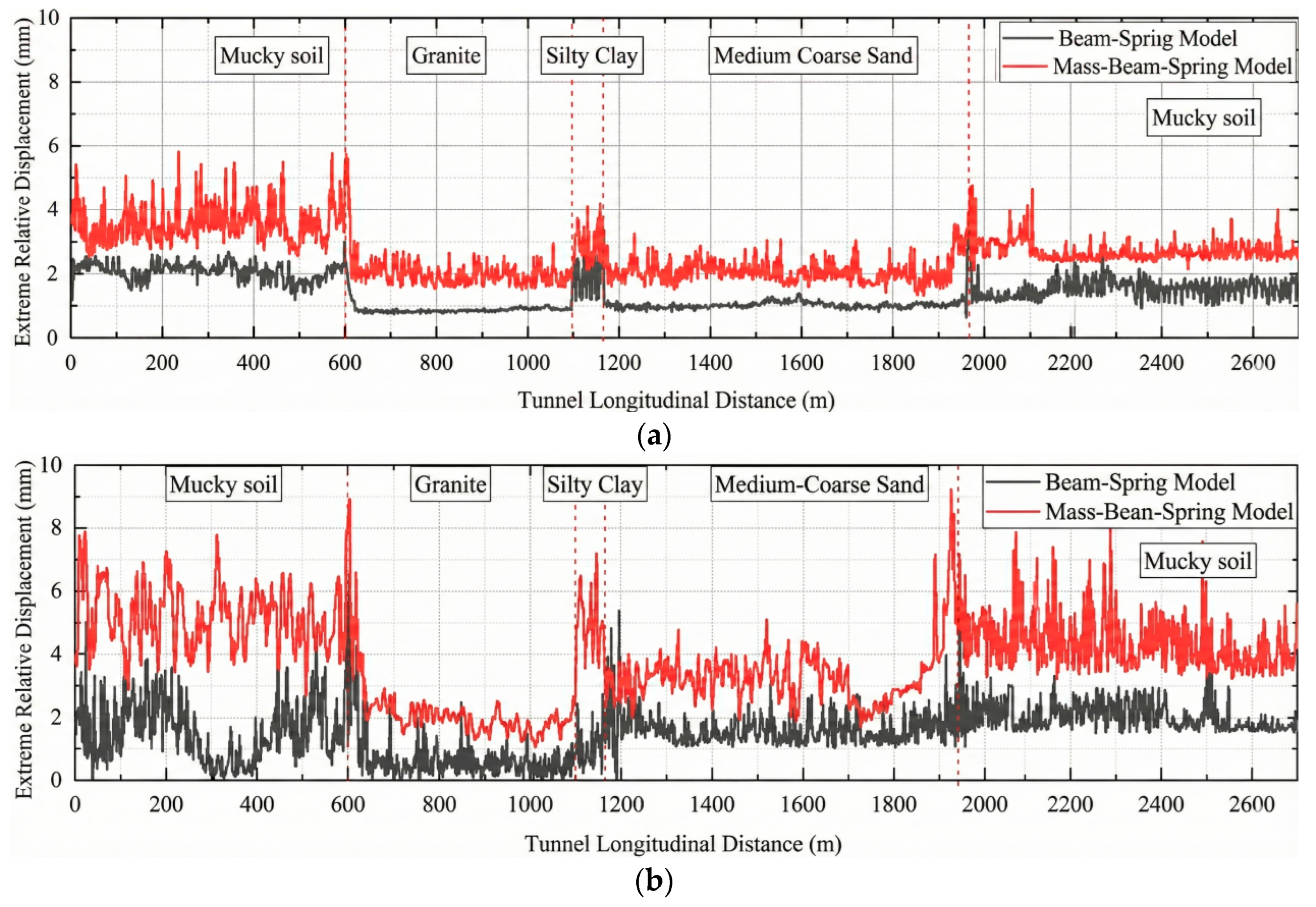
This section presents a comparative analysis of the envelope curves for the peak longitudinal relative displacements and maximum segment joint openings calculated using both the beam–spring model and the mass–beam–spring model. The objective is to investigate the influence of different ground motion input methods on the structural dynamic response.

The segment joint opening is defined as the longitudinal displacement difference between the left end of the right ring and the right end of the left ring. The relative displacement is defined as the absolute value of the difference in displacement time histories at 2 m intervals (corresponding to the nodal spacing) along the longitudinal direction of the tunnel.

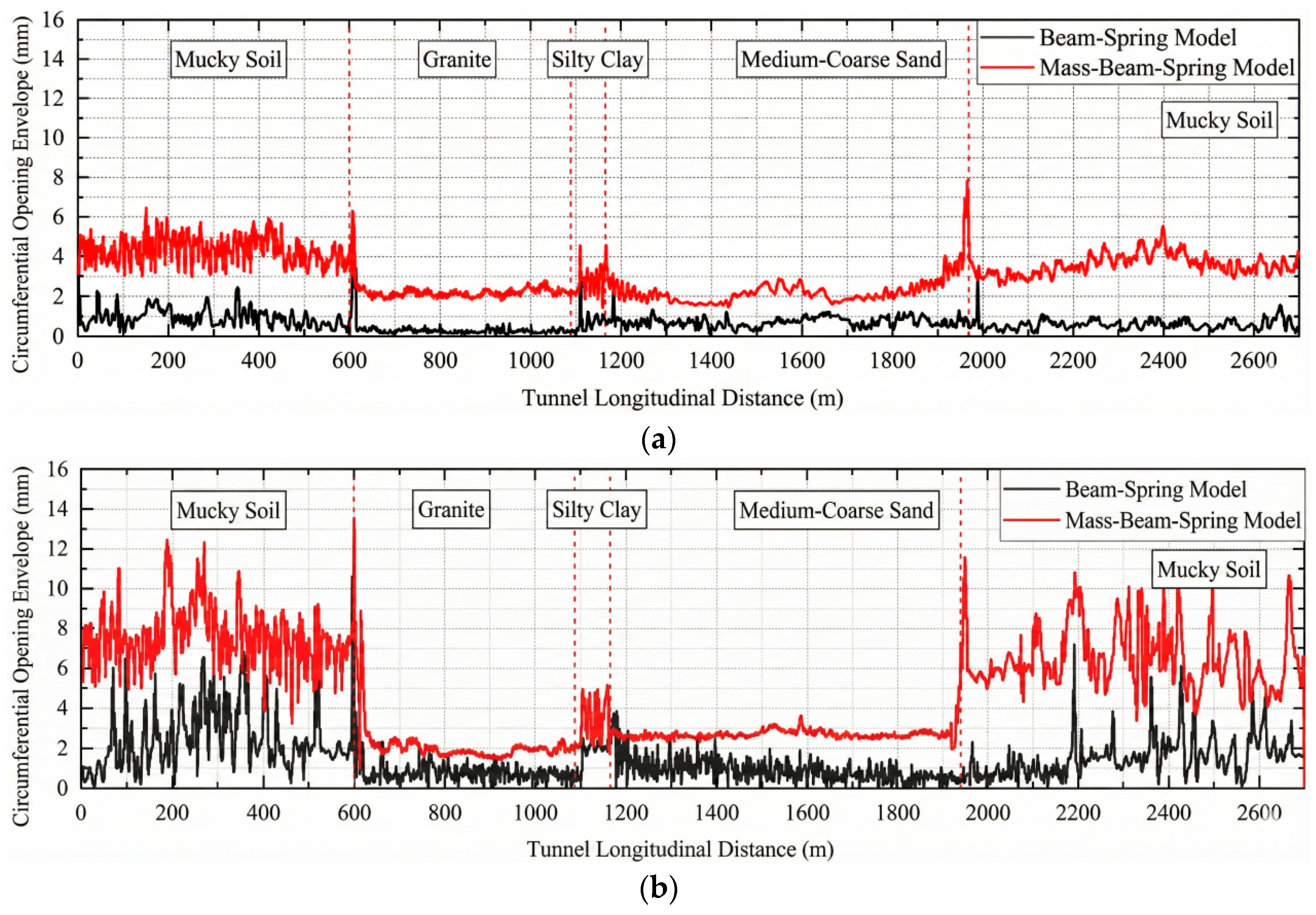
Figure 8a,b and Figure 9a,b present the envelope curves for the peak relative displacements and maximum segment joint openings of the two models under longitudinal and tri-directional input conditions. The black curves represent the results from the beam–spring model, while the red curves denote those from the mass–beam–spring model. It can be observed that both models exhibit relatively stable responses when the tunnel traverses homogeneous strata, whereas distinct abrupt response changes occur at the boundaries of surrounding rocks. The peak increments are primarily located at the 600 m, 1100 m, and 1964 m marks, which is consistent with the previously analyzed locations of internal force mutations. This indicates that abrupt changes in surrounding rock stiffness have a significant governing effect on the longitudinal dynamic response of the structure.

In terms of overall trends, the two models represent consistent characteristics regarding the locations of peak responses, particularly at the geological interfaces where surrounding rock properties undergo abrupt changes (e.g., at 600 m, 1100 m, and 1964 m). However, regarding the magnitude of response, the results calculated by the mass–beam–spring model are significantly larger than those of the beam–spring model. The fundamental reason for this discrepancy lies in the different model structures: by introducing soil mass points and their interaction springs, the mass–beam–spring model explicitly accounts for the additional inertial forces of the soil, thereby significantly amplifying the structural dynamic response. Furthermore, the substantial parameter differences in soil mass points, soil–structure springs, and shear springs at the soft–hard rock interfaces further enhance the amplitude of response mutations. Therefore, compared to the beam–spring model, the mass–beam–spring model can account for the dynamic amplification effects under complex geological conditions, particularly at the transition zones between soft and hard surrounding rocks.

The distribution of relative displacements between rings, as shown in Figure 8, follows a similar pattern to the internal forces. In the soft mucky soil sections, the MBSM predicts significantly larger and more fluctuating relative displacements compared to the smoother predictions of the BSM. This confirms that the inertial forces of the heavy soft soil mass cause not only stress concentration but also amplified differential deformation between tunnel segments.

Table 8. Maximum relative displacement of tunnel segments.

Seismic Input Direction	Longitudinal	Tri-Directional (1:0.85:0.65)
Max. Relative Displacement of BSM (mm)	2.992	6.798
Max. Relative Displacement of MBSM (mm)	5.726	9.221

summarizes the peak data from Figure 8a,b. Under tri-directional ground motion input, the maximum relative displacement of the mass–beam–spring model is 9.221 mm, which is 1.36 times that of the beam–spring model (6.798 mm). Under longitudinal input, the maximum relative displacement of the mass–beam–spring model reaches 5.726 mm, which is 1.91 times that of the beam–spring model (2.992 mm).

Table 9. Maximum segment joint opening of tunnel segments.

Seismic Input Direction	Longitudinal	Tri-Directional (1:0.85:0.65)
Max. segment joint opening of BSM (mm)	4.176	11.641
Max. segment joint opening of MBSM (mm)	7.788	13.55

summarizes the peak data from Figure 9a,b. Under tri-directional ground motion input, the maximum joint opening calculated by the mass–beam–spring model reaches 13.55 mm, representing an increase of approximately 16.4% compared to the 11.64 mm of the beam–spring model. Notably, this value approaches the waterproofing limit (15 mm) required by the code. Under longitudinal input, the maximum joint opening of the mass–beam–spring model is also significantly larger, being approximately 1.16 times that of the beam–spring model.

Furthermore, the relative displacements and joint openings of both models under tri-directional input are significantly higher than those under longitudinal unidirectional input. This indicates that the multi-directional coupling effects induced by tri-directional ground motions further amplify the structural dynamic response. These results suggest that in high-intensity seismic zones or under complex ground motion characteristics, neglecting transverse components may lead to a significant underestimation of joint deformation and damage risks.

4.3. Limitations and Scope of Applicability

While the comparative study provides valuable insights into the seismic response of shield tunnels, the limitations of the numerical modeling approach must be acknowledged to define the scope of applicability for the conclusions:

The soil–structure interaction is simulated using the equivalent linearization method. Although the spring stiffness (K) and damping (C) are updated based on the effective shear strain to account for material nonlinearity, the model essentially behaves as a linear elastic system within the time-history integration. It does not employ fully nonlinear elastoplastic constitutive models. Consequently, the model cannot simulate plastic failure, permanent ground deformation, or soil liquefaction.

Therefore, the conclusions drawn in this study are applicable to the Design Basis Earthquake level (in this case, PGA = 0.15 g), where the soil response is dominated by stiffness degradation rather than plastic flow. For Maximum Considered Earthquakes or extreme events where large-scale soil yielding or failure is expected, advanced elastoplastic continuum models would be required to capture the real behavior.

The proposed mass–beam–spring model is particularly recommended for long-distance tunnels traversing complex geological transitions involving soft soil layers. However, for sites with high liquefaction potential or active fault rupture zones, the current spring-based simplification may not fully represent the complex soil–tunnel interaction.

5. Conclusions

Based on the detailed comparative analysis of the beam–spring model (BSM) and the mass–beam–spring model (MBSM) under Design Basis Earthquake conditions (PGA = 0.15 g), the following conclusions are drawn regarding their applicability, similarities, and differences:

(1)

In terms of overall trends, both models demonstrate consistency in identifying the spatial locations of peak responses. The critical sections (stress concentrations) predicted by both models align perfectly with the geological interfaces where stiffness changes abruptly (e.g., at 600 m, 1100 m, and 1964 m). This indicates that both methods are effective in capturing the governing influence of geological transitions on the tunnel’s longitudinal response.

(2)

Significant discrepancies in waveform and distribution patterns are observed in soft soil strata (specifically mucky soil regions). The BSM yields relatively smooth internal force curves. In contrast, the MBSM exhibits high-frequency fluctuations and amplified responses in these regions. This divergence is attributed to the local inertial effects of the soil mass, which are explicitly modeled in the MBSM but neglected in the BSM.

(3)

The inclusion of inertial effects in the MBSM leads to generally larger internal forces, but the degree of amplification varies by force type. The difference in axial tension is substantial, with the MBSM predicting values approximately 60–90% higher than the BSM. This is due to the sensitive bilinear behavior of the segment joints under tension. The results of axial compression are fundamentally consistent, with the MBSM values increasing by only 9–14%. This suggests that the longitudinal tensile response is far more sensitive to soil inertial effects than the compressive response.

(4)

In the absence of in situ seismic monitoring data to definitively validate which model reflects the reality, the choice of model should be based on theoretical rigor and design safety. The BSM is computationally efficient and sufficient for tunnels in uniform or stiff ground where inertial effects are minimal. The MBSM, by theoretically accounting for soil–structure dynamic interaction, provides a more conservative envelope of deformations and internal forces. Therefore, it is considered more representative and safer for critical infrastructure design in complex geological conditions, particularly those involving thick, soft soil layers where dynamic amplification is a concern.

References

1. Huang, C.; Su, D.; Hu, Y.; Wang, X.; Qi, W.; Li, Q. A Brief Review of Recent Research Progresses on Shield Tunnelling in Soft Soil Stratum. Mod. Tunn. Technol. 2022, 59, 13–21. (In Chinese) [Google Scholar] [CrossRef]
2. Ge, S.; Gao, W.; Wang, Y.; Xie, Y.; Chen, X.; Wang, S. Review on Diseases, Evaluation and Treatment of Traffic Shield Tunnels in China. China Civ. Eng. J. 2023, 56, 119–128. (In Chinese) [Google Scholar] [CrossRef]
3. Yu, H.; Chen, J.; Bobet, A.; Yuan, Y. Damage Observation and Assessment of the Longxi Tunnel during the Wenchuan Earthquake. Tunn. Undergr. Space Technol. 2016, 54, 102–116. [Google Scholar] [CrossRef]
4. Chen, P.; Geng, P.; Chen, J.; Gu, W. The Seismic Damage Mechanism of Daliang Tunnel by Fault Dislocation during the 2022 Menyuan Ms6.9 Earthquake Based on Unidirectional Velocity Pulse Input. Eng. Fail. Anal. 2023, 145, 107047. [Google Scholar] [CrossRef]
5. Xin, C.; Feng, W.; Song, D.; Huang, S.; Liu, X. Seismic Damage to Non-Fault-Crossing and Fault-Crossing Tunnels: Comparative Study of the 2008 Wenchuan Earthquake (Mw 7.9) and the 2022 Menyuan Earthquake (Mw 6.7). Eng. Fail. Anal. 2024, 166, 108843. [Google Scholar] [CrossRef]
6. Apostolaki, S.; Karahan, S.; Riga, E.; Tsinidis, G.; Gokceoglu, C.; Pitilakis, K. Seismic Performance of Tunnels and Verification of Available Seismic Risk Models for the 2023 Kahramanmaraş Earthquakes. Tunn. Undergr. Space Technol. 2025, 156, 106185. [Google Scholar] [CrossRef]
7. Yu, H.; Yuan, Y.; Bobet, A. Seismic Analysis of Long Tunnels: A Review of Simplified and Unified Methods. Undergr. Space 2017, 2, 73–87. [Google Scholar] [CrossRef]
8. Hatzigeorgiou, G.D.; Beskos, D.E. Soil–Structure Interaction Effects on Seismic Inelastic Analysis of 3-D Tunnels. Soil Dyn. Earthq. Eng. 2010, 30, 851–861. [Google Scholar] [CrossRef]
9. Li, Y.; Zhao, M.; Xu, C.; Du, X.; Li, Z. Earthquake Input for Finite Element Analysis of Soil-Structure Interaction on Rigid Bedrock. Tunn. Undergr. Space Technol. 2018, 79, 250–262. [Google Scholar] [CrossRef]
10. Haiyang, Z.; Xiaoxiong, L.; Kai, Z.; Mingluqiu, H. Dynamic Sub-Structure Method for Longitudinal Seismic Response of Large-Diameter Shield Tunnel through the Complex Strata. Tunn. Undergr. Space Technol. 2025, 163, 106680. [Google Scholar] [CrossRef]
11. Miao, Y.; Yao, E.; Ruan, B.; Zhuang, H. Seismic Response of Shield Tunnel Subjected to Spatially Varying Earthquake Ground Motions. Tunn. Undergr. Space Technol. 2018, 77, 216–226. [Google Scholar] [CrossRef]
12. Zhou, J.; Cui, J.; Dong, R.; Li, Y.; Shan, Y. Analysis on Longitudinal Dynamic Response of In-service Buried Pipelines. Earthq. Eng. Eng. Dyn. 2022, 42, 196–203. (In Chinese) [Google Scholar] [CrossRef]
13. Li, Y.; Lai, J.; Yang, Y.; Zhou, J.; Shan, Y.; Cui, J. Seismic Performance Study of Immersed Tunnel with Longitudinal Limit Device of Flexible Joint. Undergr. Space 2025, 20, 17–32. [Google Scholar] [CrossRef]
14. Yu, H.; Song, Y.; Li, Y.; Zhang, S.; Xu, L. Multi-scale method and seismic response analysis of immersed tunnels. J. Tongji Univ. 2021, 49, 807–815. (In Chinese) [Google Scholar]
15. Wu, J.; Xu, A. Study on seismic response of soil for immersed tunnels using multi-mass-spring model. J. Guangzhou Univ. 2009, 8, 68–72. (In Chinese) [Google Scholar]
16. Yuan, Y.; Zhang, Y.; Song, S.; Li, C.; Yu, H. Analysis of traveling wave effect on simplified structural model of immersed tunnel. In Proceedings of the 2017 Academic Annual Meeting of China Civil Engineering Society, Changsha, China, 19–22 October 2017; China Civil Engineering Society: Beijing, China, 2017; p. 15. (In Chinese) [Google Scholar]
17. Wang, M.; Liang, Q.; Huang, Y.; Li, Y.; Yang, C. Study on Seismic Response Characteristics of Immersed Tube Tunnels with Longitudinal Limit Device. Mod. Tunn. Technol. 2023, 60, 106–115. (In Chinese) [Google Scholar] [CrossRef]
18. Zhou, J.; Cui, J.; Li, Y.; Shan, Y.; Donà, M.; Yang, K. Prediction of the Seismic Behavior and Backfilling Scheme Optimization of Immersed Tunnel Based on the Ruyifang Project. Soil Dyn. Earthq. Eng. 2023, 171, 107961. [Google Scholar] [CrossRef]
19. Gimena, F.N.; Goñi, M.; Gonzaga, P.; Valdenebro, J.V. Soil-Tunnel Interaction under the Effect Associated with the Longitudinal Direction. Structures 2024, 67, 106959. [Google Scholar] [CrossRef]
20. Zhang, S.; Yang, Y.; Yuan, Y.; Li, C.; Qiu, J. Experimental Investigation of Seismic Performance of Shield Tunnel under Near-Field Ground Motion. Structures 2022, 43, 1407–1421. [Google Scholar] [CrossRef]
21. Liu, L.; Xu, C.; Du, X.; Iqbal, K. Longitudinal Seismic Response of Shield Tunnel: A Multi-Scale Numerical Analysis. Tunn. Undergr. Space Technol. 2023, 138, 105163. [Google Scholar] [CrossRef]
22. GB 50011-2010; Code for Seismic Design of Buildings. Ministry of Housing and Urban-Rural Development of the People’s Republic of China (MOHURD); Architecture & Building Press: Beijing, China, 2010.
23. Chen, P.; Geng, P.; Chen, J.; Yang, Q. Deformation-Based Longitudinal Equivalent Stiffness Beam Model for Shield Tunnel and Its Application in Seismic Deformation Method. Undergr. Space 2024, 17, 280–299. [Google Scholar] [CrossRef]
24. GB 50909-2014; Code for Seismic Design of Urban Rail Transit Structures. National Standard: Beijing, China, 2010.
25. Xi, Z. Longitudinal Seismic Performance Analysis of Underwater Shield Tunnel and Research on SMA Flexible Damping Joint. Master’s Thesis, Guangzhou University, Guangzhou, China, 2017. (In Chinese) [Google Scholar]
26. Hancock, J.; Watson-Lamprey, J.; Abrahamson, N.A.; Bommer, J.J.; Markatis, A.; Mccoyh, E.; Mendis, R. An Improved Method of Matching Response Spectra of Recorded Earthquake Ground Motions Using Wavelets. J. Earthq. Eng. 2006, 10, 67–89. [Google Scholar] [CrossRef]
Figure 1. Schematic diagram of the beam–spring model.
Buildings 16 00417 g001
Figure 2. Schematic diagram of the mass–beam–spring model.
Buildings 16 00417 g002
Figure 3. (a). Constitutive relation of inter-ring tension–compression asymmetric nonlinear springs. (b) Constitutive relation of inter-ring rotational nonlinear springs.
Buildings 16 00417 g003
Figure 4. The distribution of soil layers.
Buildings 16 00417 g004
Figure 5. Acceleration time histories of artificial seismic waves.
Buildings 16 00417 g005
Figure 6. (a). Envelope of maximum axial tension at the segment mid-section under longitudinal seismic input. (b). Envelope of maximum axial tension at the segment mid-section under tri-directional seismic input.
Buildings 16 00417 g006
Figure 7. (a) Envelope of maximum axial compression at the segment mid-section under longitudinal seismic input. (b) Envelope of maximum axial compression at the segment mid-section under tri-directional seismic input.
Buildings 16 00417 g007
Figure 8. (a) Envelope of maximum longitudinal relative displacement under longitudinal seismic input. (b) Envelope of maximum longitudinal relative displacement under tri-directional seismic input.
Buildings 16 00417 g008
Figure 9. (a) Envelope of maximum segment joint opening under longitudinal seismic input. (b) Envelope of maximum segment joint opening under tri-directional seismic input.
Buildings 16 00417 g009