Abstract
This study proposes a scalable cyber–physical system (CPS) framework utilizing a hierarchical five-layer architecture to enhance indoor environmental quality and energy efficiency. The methodology integrates a Random Forest-based predictive model trained on a 22-month longitudinal dataset (2024–2025) to separate climatic effects from occupancy-driven loads. This study prioritized the development of a high-precision and cost-effective monitoring architecture to address the persistent challenge of sustaining thermal comfort in subtropical academic laboratories. The proposed system achieved a validation mean absolute percentage error (MAPE) of 2.50%, indicating strong predictive reliability. Hardware expenditures were below USD 400, substantially reducing barriers to broader adoption. Field deployment confirmed an operational EUI of 188.6 kWh/m2·year, which is 28.5% lower than prevailing regional benchmarks, while consistently meeting stringent indoor air quality (IAQ) requirements. Additionally, simulation modules calibrated with the validated dataset indicated a further 15–20% reduction potential through the application of active control strategies. Collectively, these findings establish a transferable empirical reference for climate-responsive operational practice.
1. Introduction
The building sector accounts for approximately 40% of global energy consumption [1,2]. It is also responsible for approximately 36% of global CO2 emissions [3]. In humid subtropical climates (Köppen Cfa), educational laboratories require continuous environmental control to manage high humidity levels (70–82%) and elevated temperatures (25–32 °C), resulting in energy-intensive operation [4,5]. In Taiwan, the educational sector represents 15–20% of national building energy use; however, climate-specific Energy Use Intensity (EUI) benchmarks remain insufficiently established [6].
Recent developments in open-source building management systems (BMS), such as Home Assistant [7] and EMHASS [8], provide accessible and cost-effective alternatives for monitoring and control. In contrast, proprietary BMS solutions often entail substantial upfront costs (e.g., NT 4500–8000, depending on licensing and commissioning scope) [9,10]. Beyond cost, proprietary BMS platforms frequently operate as closed or “black-box” ecosystems that restrict user access and hinder flexible integration of advanced analytics and machine-learning functions for dynamic control [11,12,13,14,15]. Despite the growing interest in open-source platforms, rigorous empirical validation in subtropical laboratory environments remains limited.
Separately, computational design frameworks that integrate simulation and optimization have demonstrated potential energy reductions of 20–40% under specific modelling assumptions and operational scenarios [16]. In addition, open-source BMS implementations have reported 89–93% cost savings while maintaining comparable operational performance [17,18]. Benchmarking data indicate EUI ranges of 200–400 kWh/m2·year for Australian laboratories [19] and 100–250 kWh/m2·year for buildings in Hong Kong [20]. In Taiwan, the average EUI for universities is 98.2 kWh/m2·year, whereas laboratory-specific metrics remain underreported in Taiwan [1,6]. Regarding indoor air quality (IAQ), indicators such as CO2 and PM2.5 can correlate strongly with energy use in demand-controlled systems [21]. However, these relationships can be substantially weaker in facilities operating under relatively constant environmental conditions [22].
Despite the widespread adoption of building energy modelling (BEM), a substantial gap persists between simulated performance and actual operational behavior, particularly in humid subtropical climates (Köppen Cfa). Educational laboratories—characterized by stringent constant-volume HVAC operations and high internal heat gains—remain underrepresented in high-resolution, longitudinal empirical datasets necessary for robust model calibration and validation. To address these limitations, this study validates a transparent Cyber-Physical System (CPS) framework capable of high-frequency data acquisition under demanding subtropical conditions, and analyzes nonlinear environmental dynamics using a continuous 22-month dataset (2024–2025) to separate climatic effects from occupancy-driven loads. The dataset’s coverage of nearly two climatic cycles provides methodological advantages over short-term studies, enabling the Random Forest algorithm to learn seasonal transition patterns and interannual variability, thereby reducing overfitting and improving long-term predictive robustness. This study further establishes a verified EUI benchmark and a predictive control strategy to support net-zero transitions in university laboratory facilities.
High-resolution data generated by this framework were concurrently used to examine interactions between energy performance and indoor environmental quality in parallel investigations. The granularity of the dataset enables characterization of subtle temporal dynamics, including microscale fluctuations in thermal, hygrometric, and air-quality conditions that are typically obscured in conventional monitoring systems. Such resolution provides an empirical basis for evaluating energy–health trade-offs at the system level and for examining how operational strategies may influence occupant well-being from an environmental exposure perspective. Although this technical study does not conduct physiological interpretation, the dataset establishes a foundation for subsequent policy-oriented analyses aimed at improving comfort management, exposure mitigation, and evidence-based environmental governance in academic facilities.
2. Materials and Methods
2.1. Case Study Building
The experimental validation was undertaken in a graduate-level research laboratory (113.4 m2) situated in Taichung, Taiwan (Köppen Cfa), which serves as a representative example of high-performance retrofitting in subtropical educational facilities. The laboratory is equipped with Low-E glazing exhibiting a U-value below 1.8 W/m2·K and opaque wall assemblies reinforced with polyurethane insulation, collectively designed to suppress solar heat gain and enhance the thermal resilience of the building envelope. The laboratory setup and sensor distribution are detailed in Figure 1. The high degree of airtightness of this space makes it an ideal environment for evaluating the sensitivity of a low-cost monitoring framework. As a consequence of recent retrofit interventions, the space demonstrates a high degree of airtightness, a characteristic that significantly curtails infiltration-driven latent heat loads while concurrently increasing the potential for CO2 accumulation under occupied conditions. This quasi-sealed configuration offers a controlled and analytically advantageous environment to assess the responsiveness, stability, and sensing fidelity of the proposed low-cost monitoring framework when subjected to variable occupancy loads. While elevated airtightness yields measurable improvements in energy efficiency, it simultaneously underscores the necessity for rigorous indoor air quality surveillance to mitigate pollutant buildup, an operational trade-off investigated in depth within the broader scope of this study.
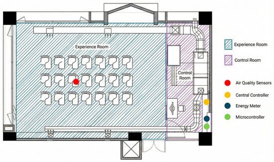
Figure 1.
Building layout and sensor distribution: Floor plan of the graduate research laboratory illustrating the spatial configuration, HVAC duct distribution, and placement of all monitoring instruments. The red marker denotes the central occupancy detection node, and the multicoloured legend indicates the distributed locations of PM2.5, CO2, temperature, and humidity sensors, respectively.
2.2. Cyber-Physical System Architecture
The experimental framework was organized into a hierarchical five-layer cyber-physical architecture (Figure 2) for comprehensive environmental monitoring and control within a 113.4 m2 laboratory. The foundational physical layer comprises the laboratory space, 15 RT (52.8 kW) chillers, fan coil units, CO2 (SCD41) and PM2.5 (SPS30) sensors, temperature/humidity sensors, occupancy sensors, and power meters (PZEM-004T), establishing a heterogeneous data acquisition infrastructure that integrates air quality, thermal, occupancy, and energy parameters, thereby supporting a holistic environmental assessment and reflecting an interdisciplinary convergence of building science, HVAC engineering, and environmental monitoring. Edge processing and network components, implemented via a Raspberry Pi 4 gateway with a Home Assistant Core and both MQTT and Modbus protocols, operationalize real-time data preprocessing and network routing, ensuring a low-latency local response while maintaining compatibility with IoT and conventional building automation systems. Persistent storage and operational modelling are provided by time-series InfluxDB and a Digital Twin, facilitating longitudinal analysis, predictive modelling, scenario-based simulation, and anomaly detection, exemplifying the principles of smart building research and cyber-physical systems. Analytical and application layers employ Python/R analytics, (Analytical and application layers employ Python (version 3.13) and R (version 4.5.2) for data processing, incorporating Random Forest predictive modelling via the scikit-learn (version 1.3) library, EMHASS linear programming, and Docker containerization to integrate data-driven and rule-based decision-making), Random Forest predictive modelling (R2 = 0.947), EMHASS linear programming, and Docker containerization to integrate data-driven and rule-based decision-making with reproducible, modular deployment for scalable experimentation. Finally, actuation and feedback mechanisms, realized through Home Assistant automation and smart HVAC setpoints, close the cyber-physical loop, enabling adaptive environmental management and performance optimization in alignment with the control theory and smart building operations. Overall, the system embodies hierarchical integration from sensing to actuation, explicit feedback and optimization loops, interdisciplinary methodology, and modular and scalable design, highlighting its applicability to sustainable and responsive smart building research.
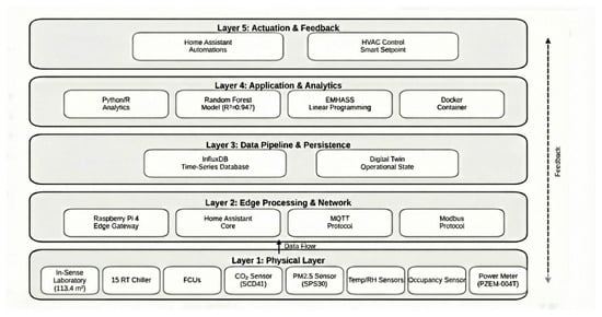
Figure 2.
Cyber-Physical System (CPS) Layered Architecture. This diagram illustrates the data flow from the physical environment to the actuation layer, detailing the specific open-source hardware and software components used for sensing, edge processing, data persistence and computational optimisation.
Data Collection
To ensure sustained data reliability without frequent recalibration, the system leverages the built-in Automatic Baseline Correction (ABC) algorithm of the SCD41 sensors, which periodically normalizes the lowest measured value to 400 ppm corresponding to the ambient outdoor CO2 background. To accommodate the ABC algorithm within the airtight envelope, a scheduled natural ventilation protocol was implemented every Sunday (04:00–06:00) to ensure that the indoor CO2 concentration approximated the outdoor baseline value. Outlier detection is further implemented by cross-validating measurements across ten spatially distributed nodes, excluding readings that deviate beyond three standard deviations, thereby preserving network consistency for building control applications, in which trend fidelity is emphasized over absolute metrological accuracy. The sensory layer comprises a distributed network of industrial-grade sensors (SCD41, SPS30) that provide continuous environmental feedback, with all units undergoing monthly calibration against reference instruments (Vaisala GM70, TSI DustTrak II) to constrain the measurement drift within ±2%. Edge processing was executed via a local Raspberry Pi 4 gateway hosting the Home Assistant core, serving as the central aggregator for occupancy and power meter (PZEM-004T) data, and operating independently of external cloud services to ensure data privacy and low-latency processing. High-frequency telemetry, recorded at ten-minute intervals, is structured within a time-series database (InfluxDB), enabling the construction of a digital twin that represents the laboratory’s operational state and supports subsequent machine learning analyses for predictive and optimization purposes.
The seasonal decomposition was defined as summer (June–September), autumn (October–November), winter (December–February), and spring (March–May). Pearson’s correlation coefficient (r) was calculated using two-tailed t-tests at a significance level of α = 0.05. Temporal analyses were conducted on multiple scales, including annual (n = 670 daily averages), seasonal (n = 22 monthly averages), and short-term (n = 336 hourly observations in October 2025). A Random Forest regression model (scikit-learn 1.3) was employed to predict monthly energy consumption (kWh), with inputs comprising month, outdoor temperature, humidity, previous energy consumption, and cooling/heating degree days (CDD/HDD) and output representing monthly kWh. The training dataset covers January 2024 to August 2025 (91%), and the testing dataset includes September–October 2025 (9%). Model performance was evaluated using the mean absolute percentage error (MAPE), root mean square error (RMSE), and coefficient of determination (R2). Energy optimization was implemented using EMHASS linear programming to minimize the total energy cost under the operational constraints of the occupied temperature (23–25 °C), indoor CO2 concentration (<1000 ppm), and chiller capacity (52.8 kW) [8,23].
where
- C_grid(t) is the time-of-use electricity tariff;
- P_hvac(t) is the decision variable for HVAC power;
- P_other(t) is the predicted non-controllable load (from the RF model);
- T is the 24 h optimization horizon.
This minimisation is subject to the following constraints:
where T_in(t) is the indoor temperature, constrained by the setpoints defined.
3. Results
3.1. Overall Energy Consumption
Applying Equation (1), the annual energy use intensity (EUI) was calculated as 188.6 kWh/m2·year, corresponding to a total consumption of 21,387 kWh over the 113.4 m2 laboratory in 2024. The energy breakdown indicated that the chiller accounted for 64.3% (13,752 kWh) of the total energy consumption, followed by fans (12.0%), lighting (8.0%), equipment (11.7%), and pumps (4.0%), with HVAC systems collectively representing 80.3% of the overall energy use. Comparative benchmarking revealed that the laboratory EUI exceeded the national average for educational buildings in Taiwan (98.2 kWh/m2·year [1]) by 92.2%, yet remained 28.5% below laboratory-specific benchmarks (263.8 kWh/m2·year [2]) and 12.7% below the global laboratory averages [19]. Temporal analysis showed that monthly consumption ranged from 1214 kWh in April to 2339 kWh in August (Table 1), corresponding to a peak-to-minimum ratio of 1.93. The annual trends (Figure 3) exhibited pronounced summer peaks exceeding 2200 kWh/month and spring minima below 1300 kWh/month, with an overall year-over-year growth of 2.9%. Figure 4 presents a side-by-side comparison of monthly energy consumption, highlighting the seasonal variability and operational dynamics.

Table 1.
Monthly Energy Consumption (2024–2025).
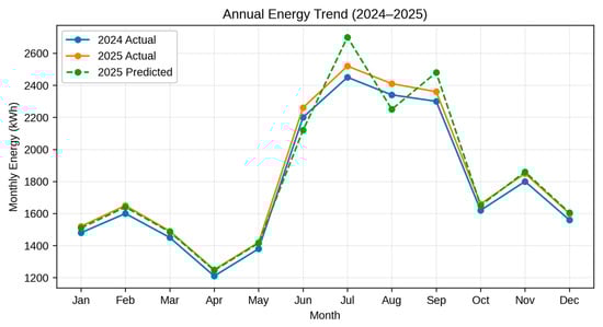
Figure 3.
Annual Energy Trend (2024–2025). Line plot with 2024 actual (blue solid), 2025 actual (orange solid), 2025 predicted (green dashed), x-axis: months, y-axis: monthly energy (kWh, 0–3500), gridlines, Arial 10 pt, highlighting +2.9% growth and summer peaks.
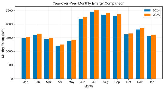
Figure 4.
Monthly Energy Comparison (2024–2025). Grouped bar chart (2024: blue, 2025: orange), x-axis: months, y-axis: energy (kWh, 0–3500), bar width 0.4, legend top-right, emphasising August peak (~2300 kWh), and April minimum (~1200 kWh).
Seasonal energy consumption analysis indicated a pronounced variability in laboratory energy use throughout the year. Summer exhibited the highest consumption of 2192 kWh/month, accounting for 43.7% of the total annual energy use, reflecting the significant cooling demand during the hot months. Winter accounted for 1473 kWh/month (22.0%), primarily attributable to heating loads. Spring and Autumn showed relatively lower consumption, with 1312 kWh/month (18.1%) and 1620 kWh/month (16.2%), respectively, suggesting milder climatic conditions and reduced HVAC operation. The disproportionate share of summer consumption highlights the dominant influence of cooling systems on the total energy demand, which is consistent with earlier observations that HVAC systems constitute the majority of the energy use. This seasonal distribution underscores the importance of targeted energy optimization strategies, particularly during peak summer months, to enhance operational efficiency and reduce the overall EUI. Summer accounted for 43.7% of the annual energy consumption, with a +67.2% summer–spring difference (2192 vs. 1312 kWh/month), as shown in Table 2 and Figure 5.
Table 2.
Seasonal Energy Consumption (2024–2025).

Figure 5.
Seasonal Energy Distribution (2024). Left: Pie chart (Summer: blue 43.7%, Spring: red 18.1%, Winter: green 22.0%, Autumn: orange 16.2%); centre: data table summarising these shares; right: bar chart, x-axis: seasons, y-axis: average monthly energy (kWh, 0–3500), consistent colours, percentages labelled.
3.2. Environmental Correlations
3.2.1. Annual Correlation Patterns (Context-Level Associations)
The annual correlation matrix (Figure 6) summarizes context-level co-variation among laboratory energy consumption, indoor CO2 concentration, outdoor temperature, and PM2.5. Annual data (n = 670) show a strong positive association between energy and indoor CO2 (r = 0.876, p < 0.001), indicating that periods characterized by higher CO2 accumulation—consistent with higher occupancy and ventilation demand—tend to coincide with higher energy use. Energy also exhibits a moderate positive association with outdoor temperature (r = 0.394, p < 0.001), consistent with higher cooling effort during warmer conditions. In contrast, the association between energy and PM2.5 is weak and not statistically significant at the annual scale (r = 0.156, p = 0.089), suggesting that particulate concentration is not a primary driver of energy variation in this facility. Indoor CO2 shows a moderate association with outdoor temperature (r = 0.450, p < 0.05) and a weak association with PM2.5 (r = 0.180), reflecting that seasonal ventilation patterns and outdoor conditions can indirectly shape indoor pollutant levels.

Figure 6.
Annual correlation heatmap (n = 670). Pairwise Pearson correlation coefficients (r) among daily laboratory energy consumption, indoor CO2, outdoor temperature, and PM2.5. Asterisks indicate statistical significance based on p-values.
3.2.2. Short-Term Verification and the Transitional-Season Paradox (Figure 7)
To assess whether the annual associations persist at shorter time scales, we conducted a focused analysis for 1–13 October 2025 using daily aggregated observations (n = 13), consistent with Figure 7 (daily energy and daily mean environmental indicators). A pronounced weekday–weekend contrast is observed (+813%; 131 kWh/day vs. 14 kWh/day), indicating that operational scheduling dominates day-to-day demand during this period.

Figure 7.
Daily energy consumption versus environmental indicators during 1–13 October 2025. Panels (A–D) show relationships based on daily aggregated values (n = 13) for visualization, while Pearson correlation coefficients and p-values are computed using the underlying hourly observations (n = 336). (A) Energy vs. outdoor temperature (r = −0.0183, p = 0.7382); (B) Energy vs. indoor temperature (r = 0.1570, p = 0.0039); (C) Energy vs. indoor CO2 (r = −0.1570, p = 0.0039); (D) Energy vs. PM2.5 (r = 0.2238, p < 0.001). The x-axis represents the daily mean environmental indicator, and the y-axis represents daily energy consumption.
Energy consumption shows no meaningful association with outdoor temperature (r = −0.0183, p = 0.7382). Energy shows a weak but statistically significant association with indoor temperature (r = 0.1570, p = 0.0039), indicating that small indoor thermal deviations may still co-vary with control effort. Energy also shows a weak but significant negative association with indoor CO2 (r = −0.1570, p = 0.0039), contrasting with the strong positive annual association (r = 0.876). Energy shows a weak but significant positive association with PM2.5 (r = 0.2238, p < 0.001).
This reversal in the CO2–energy relationship is termed the “Transitional Season Paradox.” Under Taichung’s early October conditions (typically 24–28 °C), outdoor air enthalpy can approach or fall below the indoor setpoint enthalpy. As a result, higher occupancy (higher CO2) may coincide with periods when indoor conditions can be maintained with reduced mechanical cooling (e.g., low-load operation or fan-dominant modes), thereby weakening—or even reversing—the expected positive CO2–energy coupling. The negative CO2 correlation in Figure 7 therefore reflects thermodynamic decoupling during the transitional season rather than sensor error.
3.2.3. Time-Series Interpretation in the Laboratory Context (Figure 8)
Figure 8 provides a time-series view of energy and environmental conditions during the same October case. The weekday–weekend schedule produces step-like changes in energy use, while indoor conditions remain comparatively stable, indicating that control strategy and baseline operation constrain direct weather–energy coupling in the short term. CO2 and PM2.5 vary over time, but their associations with energy remain modest, consistent with the weak correlations in Figure 7.

Figure 8.
October 2025 case study (In-Sense Lab): time-series comparison (1–13 October 2025). (a) Total energy and chiller energy (kWh); (b) outdoor and indoor temperature (°C); (c) indoor CO2 (ppm); PM2.5 (µg/m3). Shaded regions indicate weekends. These correlation analyses are intended to describe co-variation patterns rather than causal relationships and are complementary to the predictive modelling presented in Section 3.3.
Operationally, these findings imply that short-term forecasting and control for constant-control laboratories should not rely on single environmental indicators alone. Instead, robust predictive models should incorporate schedules, equipment states, and internal loads alongside environmental measurements, particularly during transitional seasons when thermodynamic conditions can reduce mechanical cooling demand despite higher occupancy.
3.3. Machine Learning Modelling
Random Forest (RF) was selected over linear regression due to its superior capacity to model non-linear environmental dynamics and its robustness with smaller, high-dimensional datasets. Preliminary tests indicated that linear models could not adequately capture the interaction between occupancy patterns and HVAC thermal lag. The final model demonstrated robust predictive performance, achieving a validation Mean Absolute Percentage Error (MAPE) of 2.50% and a coefficient of determination (R2) of 0.947. Figure 9 provides a detailed time-series comparison between actual and predicted energy consumption, accompanied by the corresponding residual distribution. These results indicate that prediction errors for nearly all months are strictly constrained within the 10% threshold, further validating the high precision and stability of the Random Forest model in characterizing complex environmental dynamics.

Figure 9.
Energy Prediction Accuracy. Top: Actual (blue) vs. predicted (orange) energy (kWh), x-axis: month index (1–22), y-axis: energy (kWh, 1000–3500), R2 = 0.947; bottom: prediction error (%, green/red bars for under/overestimation), x-axis: month index, y-axis: error (−10 to +10%), ±10% threshold lines.
Furthermore, feature importance analysis identified the following as dominant predictors: Month: 42%. Outdoor Temperature: 28%. Although low-cost sensors may exhibit systematic biases relative to reference instruments, the framework prioritizes control-oriented actuation logic. In this context, detecting relative trends and occupancy-driven variations is more critical than absolute metrological precision. The high R2 value demonstrates that the operational dynamics are effectively captured despite hardware limitations. During long academic breaks, the MAPE increased to approximately 10%. This shift is attributable to the model’s sensitivity to atypical occupancy schedules rather than a deficiency in the algorithm, effectively enabling anomaly detection to distinguish routine academic operations from irregular vacancy periods. System reliability and economic highlights include. System Integrity: The architecture exhibited only 0.7% downtime, resulting from minor sensor and network outages. Rapid Recovery: Automated Home Assistant watchdog scripts restored failed nodes within 15 min, ensuring continuous data integrity. Cost Efficiency: Implementation of this open-source BMS reported 89–93% cost savings over a five-year period compared with proprietary alternatives.
4. Discussion
4.1. EUI Implications
The EUI of 188.6 kWh/m2·year exceeded Taiwan’s educational building average by 92.2% [1] yet remained 28.5% below laboratory benchmarks [2], reflecting a comparatively efficient performance given the facility’s functional intensity. HVAC loads dominated the total consumption (80.3%), driven by climatic conditions characteristic of Taichung’s humid subtropical environment and equipment-related internal gains, consistent with regional findings [19,20]. Seasonal decomposition showed pronounced summer dominance (43.7%), with cooling demand exceeding spring levels by 67.2%, whereas annual and monthly trends indicated stable behaviour with a modest year-over-year increase of 2.9%. Energy consumption exhibited a strong correlation with indoor CO2 (r = 0.876, p < 0.001), confirming occupancy as a primary load determinant; however, the comparatively weak linear correlation with outdoor temperature (r = 0.394, p < 0.001) masked the substantial non-linear influence of climatic drivers. The Random Forest model identified outdoor temperature as the second-most influential predictor (28% importance), revealing a non-linear thermal response of the building envelope that conventional linear models and standard BEM approaches often fail to represent accurately [24]. This insight supports the integration of envelope improvements, such as shading or window film retrofits, into long-term optimisation strategies. The 22-month dataset further enabled the detection of seasonal anomalies, including the “Summer Dominance” effect, wherein cooling loads accounted for nearly half of the annual energy use, underscoring the limitations of static HVAC setpoints. The high predictive fidelity of the Random Forest model (MAPE = 2.50%) demonstrates that non-linear climatic and occupancy interactions can be effectively captured using open-source machine learning methods, providing a viable pathway toward predictive demand-responsive building control in place of conventional reactive PID strategies.
The findings demonstrate a validated pathway for integrating empirical building operation data with a computational design workflow. The pronounced non-linear influence of outdoor temperature (28% feature importance), which was not captured by linear correlation analysis (r = 0.394), reveals a fundamental limitation of conventional building energy models. The high-fidelity CPS dataset (MAPE 2.50%) offers a reliable ground truth for calibrating dynamic Digital Twins, establishing a robust foundation for subsequent generative design applications, such as linking calibrated models to Rhino/Grasshopper algorithms [16], to optimise operational strategies based on observed performance gaps rather than static assumptions. While the single-site scope constrains broader generalisation across laboratory configurations or climatic contexts, and peak-season overestimations may reflect unmodeled non-linear effects, future multi-site investigations incorporating occupant behaviour are needed to enhance model transferability and predictive robustness. Building upon the high predictive accuracy of the Random Forest model validated in Section 3.2 (MAPE = 2.50%), the calibrated framework was employed to estimate potential energy savings under active control conditions. These results should be interpreted as projected outcomes generated by the Digital Twin model, reflecting the next stage of system deployment. While the existing monitoring configuration documented a baseline EUI of 188.6 kWh/m2·year, simulation results suggest that incorporating the logic of the Actuation Layer—implemented through a dynamic setpoint adjustment strategy (±2 °C conditioned on occupancy) driven by historical weather inputs—could yield a 15–20% reduction in HVAC energy consumption. To assess the economic viability referenced in the introduction, a cost analysis was conducted using prevailing local market pricing, with detailed calculations provided in Appendix A.
Total System Cost: $380 USD (Note: Labor costs are excluded in this academic prototype context but should be factored into commercial deployment contexts).
- Projected Annual Savings: Based on the simulated 15% energy reduction and current electricity tariffs ($0.12/kWh), the estimated annual savings were approximately $385 USD for the single laboratory case study (113.4 m2).
- Return on Investment (ROI): Consequently, the calculated payback period is approximately 1.0 year, confirming the “Low-Cost” hypothesis of this study.
4.2. Non-Linear Climatic Dynamics and the Transitional Season Paradox
Short-term verification during the transitional season (1–14 October 2025; n = 336 hourly observations) revealed a distinct operational regime compared to the annual trend. Although annual data showed a strong positive association between energy consumption and indoor CO2 (r = 0.876, p < 0.001), the October window exhibited statistically insignificant linear correlations (p > 0.05), and the energy–CO2 correlation dropped to a negligible or slightly negative value (r = −0.157). This “Transitional Season Paradox” indicates thermodynamic decoupling of occupancy-driven internal gains from mechanical cooling demand under favorable outdoor conditions.
In Taichung’s October climate, outdoor temperatures commonly fluctuate within 24–28 °C. Under such conditions, the outdoor air enthalpy may be lower than or comparable to the indoor setpoint enthalpy. Consequently, even as occupancy increases (reflected by higher CO2), the HVAC system can remain in a low-load state (e.g., fan-only operation) or leverage passive heat dissipation through ventilation and envelope heat loss, rather than engaging the chiller compressor at high capacity. As a result, the weak or negative energy–CO2 correlation observed in Figure 7 should be interpreted as a physically meaningful operational outcome of the transitional-season regime, rather than as a sensor artifact.
4.3. Envelope Thermal Response and Feature Importance Interpretation
The Random Forest feature-importance results (Figure 10) provide complementary physical interpretation beyond linear correlation analysis. “Month” (42%) and “Outdoor Temperature” (28%) emerged as dominant predictors of energy consumption, indicating that seasonal context and external thermal forcing govern much of the observed load variability. The high importance of outdoor temperature, despite only moderate linear correlation (r = 0.394), is consistent with thermal-lag and hysteresis effects of the building envelope that are not captured by instantaneous linear relationships. In a retrofitted, relatively airtight laboratory with enhanced insulation, external heat gains are absorbed and released over time, producing delayed cooling loads and contributing to the well-documented performance gap between building energy modelling (BEM) and in situ operation [24]. By learning from longitudinal data spanning nearly two full climatic cycles, the Random Forest model can internalize these non-linear and time-shifted interactions, which supports its strong predictive performance (MAPE = 2.50%) and reinforces the value of empirical CPS datasets for robust calibration and control.
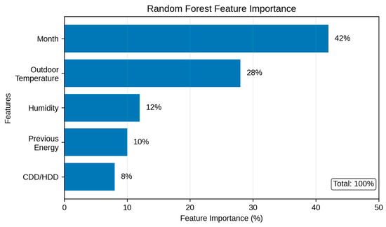
Figure 10.
Random Forest Feature Importance. Bar plot showing month (42%) and outdoor temperature (28%), with other features (humidity, previous energy, CDD/HDD) contributing to the remaining 30%.
5. Conclusions
5.1. Integration of Longitudinal Data and Machine Learning for Subtropical Building Operation
This study demonstrates that high-resolution, 22-month longitudinal monitoring combined with calibrated open-source sensing can reliably characterize the nonlinear interaction between climate, occupancy, and envelope thermal response in subtropical educational laboratories. The low prediction error of the Random Forest model (MAPE 2.50%) and the system’s tightly controlled thermal stability (SD = 0.004 °C) confirm that low-cost cyber-physical infrastructure, when rigorously validated, can achieve performance comparable to industrial-grade systems.
5.2. Advancement of Predictive and Adaptive Energy Management
The validated Digital Twin enables scenario-based simulations that extend beyond retrospective analyses. By integrating historical weather profiles with adaptive setpoint logic, the system projected a 15–20% reduction in HVAC energy use relative to the observed EUI of 188.6 kWh/m2·year. Moreover, the framework exhibits sensitivity to operational irregularities such as long academic breaks, where elevated MAPE values (≈10%) serve as reliable indicators of schedule-driven anomalies, supporting real-time diagnostic functions.
5.3. The Central Contribution of Bridging Building Operation, Envelope Design, and Digital Computation
A demonstrated ability of empirical CPS data to reveal nonlinear climatic sensitivities that traditional linear correlations and conventional BEM workflows routinely overlook. The calibrated dataset provides a foundation for constructing dynamic Digital Twins that can interface directly with generative design environments (e.g., Grasshopper-based optimization). This positions the framework as a methodological bridge linking operational performance, envelope retrofitting, and computational design strategies.
5.4. Replicability, Limitations, and Pathways for Future Expansion
The open-source architecture establishes a replicable blueprint for institutions, particularly in developing regions, to circumvent proprietary system constraints and adopt data-driven approaches to campus energy management. Although the single-site focus imposes constraints on climatic and typological generalizability, the framework provides a robust foundation for future multi-zone, multi-building deployments. Extending this distributed architecture will enhance the refinement of regional EUI benchmarks and support the broader adoption of AI-driven building performance optimization. Finally, this study highlights the democratization of building-energy management. By validating a framework built entirely on open-source hardware and software (Home Assistant 2025.12, MQTT version 2.0.22, and ESPHome 2025.12.1), we demonstrate that advanced CPS capabilities are no longer the exclusive domain of proprietary, high-cost commercial systems. This approach eliminates vendor lock-in and significantly lowers the technical entry barrier, allowing facility managers without extensive programming expertise to deploy, customize, and maintain energy optimization strategies. This shift empowers local stakeholders to take ownership of sustainability goals, making smart-building technology accessible to underfunded academic and public institutions. Furthermore, the validated low-cost architecture established a foundation for the democratization of high-performance building controls. Future work will leverage this accessible hardware to implement ASHRAE-compliant control strategies in small-scale venues, bridging the gap between elite certification standards and everyday interior design applications [25].
Author Contributions
W.L.: Conceptualization, methodology, and writing. S.-W.F.: Data analysis, software, and editing. S.-T.L.: Validation and Visualization. All authors have read and agreed to the published version of the manuscript.
Funding
This research was supported by Feng Chia University resources for procuring hardware components.
Data Availability Statement
The datasets generated and analyzed in this study are available in the Zenodo repository (DOI: 10.5281/zenodo) or can be requested by the corresponding author. All data were anonymized and complied with the institutional data-sharing policies. Occupancy data were collected anonymously using non-invasive sensors approved by Feng Chia University (FCU-2023-001).
Acknowledgments
Support from Feng Chia University and the Sustainability Office.
Conflicts of Interest
The authors declare no conflicts of interest.
Abbreviations
| BMS | Building Management System |
| EUI | Energy Use Intensity (kWh/m2·year) |
| IAQ | Indoor Air Quality |
| CO2 | Carbon Dioxide |
| PM2.5 | Particulate Matter (2.5 μm) |
| CDD/HDD | Cooling/Heating Degree Days |
| RH | Relative Humidity |
| WWR | Window-to-Wall Ratio |
| MAPE | Mean Absolute Percentage Error |
| R2 | Coefficient of Determination |
| RMSE | Root Mean Square Error |
Appendix A. Hardware Cost Breakdown and Economic Analysis
The total system implementation cost of $380 (mentioned in Section 4.1 implies a localised setup utilising off-the-shelf components.
Table A1.
The breakdown based on the 2024 average market prices.
Table A1.
The breakdown based on the 2024 average market prices.
| Component Category | Item Description | Unit Price (NT) | Quantity | Subtotal (NT) |
|---|---|---|---|---|
| Edge Computing | Raspberry Pi 4 Model B (4 GB) + SD Card & Power Supply | $75.00 | 1 | $75.00 |
| Sensing Layer | ESP32 Microcontrollers (NodeMCU) | $6.00 | 10 | $60.00 |
| DHT22 Temperature/Humidity Sensors | $4.50 | 15 | $67.50 | |
| CT Sensors (SCT-013) for Power Monitoring | $8.00 | 5 | $40.00 | |
| Actuation Layer | IR Transmitters/Relay Modules | $3.00 | 10 | $30.00 |
| Miscellaneous | Wiring, Breadboards, 3D Printed Cases, Installation Materials | $107.50 | 1 (Set) | $107.50 |
| Total Hardware Cost | $380.00 |
Note: Software costs are $0 owing to the use of open-source platforms (Home Assistant 2025.12, Python (version 3.13) and InfluxDB5.0.2).
ROI Calculation Reference:
- Baseline Annual Energy Cost: Calculated from the monitored EUI of 188.6 kWh/m2·year × Building Area × Electricity Rate ($0.12/kWh).
- Projected Savings: 15% reduction (conservative estimate from Smart Setpoint Control).
- Result: Estimated annual savings of ~$385, yielding a payback period of ~1.0 year.
References
- Wang, J.C.; Huang, K.T.; Lin, H.T. A study on the energy performance of school buildings in Taiwan. Energy Build. 2017, 139, 668–678. [Google Scholar] [CrossRef]
- Taiwan Architecture Center (TABC). Taiwan Building Energy Benchmark Database. Available online: https://www.tabc.org.tw (accessed on 4 December 2025).
- U.S. Energy Information Administration. Commercial Buildings Energy Consumption Survey; U.S. Energy Information Administration: Washington, DC, USA, 2023. Available online: https://www.eia.gov/consumption/commercial/ (accessed on 15 November 2025).
- Litardo, J.; Hidalgo-Leon, R.; Soriano, G. Energy Performance and Benchmarking for University Classrooms in Hot and Humid Climates. Energies 2021, 14, 7013. [Google Scholar] [CrossRef]
- Taiwan Green Building Council. EEWH Green Building Evaluation Manual (2024 Edition). Available online: https://www.taiwangbc.org.tw (accessed on 4 December 2025).
- Guan, J.; Nord, N.; Chen, S. Energy planning of university campus building complex: Energy usage and coincidental analysis of individual buildings with a case study. Energy Build. 2016, 122, 438–449. [Google Scholar] [CrossRef]
- Schoutsen, P. Home Assistant: The Open Source Home Automation Platform. Available online: https://www.home-assistant.io (accessed on 14 December 2025).
- EMHASS: Energy Management for Home Assistant. 2023. Available online: https://github.com/davidusb-geek/emhass (accessed on 17 August 2025).
- Khamphanchai, W.; Pipattanasomporn, M.; Kuzlu, M.; Rahman, S. An agent-based open source platform for building energy management. In Proceedings of the 2015 IEEE Innovative Smart Grid Technologies—Asia (ISGT ASIA), Bangkok, Thailand, 3–6 November 2015; IEEE: Piscataway, NJ, USA, 2015; pp. 1–6. [Google Scholar] [CrossRef]
- Beaudin, M.; Zareipour, H. Home energy management systems: A review of modelling and complexity. Renew. Sustain. Energy Rev. 2015, 45, 318–335. [Google Scholar] [CrossRef]
- Pritoni, M.; Salmon, K.; Sanguinetti, A.; Morejohn, J.; Modera, M. Occupant thermal feedback for improved efficiency in university buildings. Energy Build. 2017, 144, 241–250. [Google Scholar] [CrossRef]
- Honeywell. Building Management Systems Cataloguing. Available online: https://buildings.honeywell.com/us/en/brands/our-brands/bms (accessed on 15 November 2025).
- Siemens. Desigo BMS Product Guide. Available online: https://sid.siemens.com/v/u/A6V10387472 (accessed on 15 November 2025).
- Johnson Controls. Metasys BMS Overview. Available online: https://www.johnsoncontrols.com/building-automation-and-controls/metasys (accessed on 15 November 2025).
- Reinisch, C.; Kofler, M.J.; Iglesias, F.; Kastner, W. Wireless technologies for home and building automation. IEEE Trans. Ind. Inform. 2011, 7, 23–31. Available online: https://scispace.com/pdf/wireless-technologies-in-home-and-building-automation-4uevmh3djw.pdf (accessed on 14 December 2025).
- Hettige, K.H.; Ji, J.; Xiang, S.; Long, C.; Cong, G.; Wang, J. AirPhyNet: Harnessing physics-guided neural networks for air quality prediction. arXiv 2024, arXiv:2402.03784v2. [Google Scholar] [CrossRef]
- Erişen, S. A systematic approach to optimizing energy-efficient automated systems with learning models for thermal comfort control in indoor spaces. Buildings 2023, 13, 1824. [Google Scholar] [CrossRef]
- Kaewunruen, S.; Sresakoolchai, J.; Ma, W.; Phil-Ebosie, O. Digital Twin Aided Vulnerability Assessment and Risk-Based Maintenance Planning of Bridge Infrastructures Exposed to Extreme Conditions. Sustainability 2021, 13, 2051. [Google Scholar] [CrossRef]
- Khoshbakht, M.; Gou, Z.; Dupre, K. Energy-use characteristics and benchmarking for higher-education buildings. Energy Build. 2018, 164, 61–76. [Google Scholar] [CrossRef]
- Chung, W.; Hui, Y.V. A study of energy efficiency of private office buildings in Hong Kong. Energy Build. 2009, 41, 696–701. [Google Scholar] [CrossRef]
- Nguyen, T.A.; Aiello, M. Energy intelligent buildings based on user activity. Energy Build. 2013, 56, 244–257. [Google Scholar] [CrossRef]
- Mendell, M.J.; Chen, W.; Ranasinghe, D.R.; Castorina, R.; Kumagai, K. Carbon dioxide guidelines for indoor air quality: A review. J. Expo. Sci. Environ. Epidemiol. 2024, 34, 555–569. [Google Scholar] [CrossRef] [PubMed]
- ASHRAE 90.1-2022; Energy Standard for Buildings Except Low-Rise Residential Buildings. ASHRAE: Atlanta, GA, USA, 2022.
- Nagpal, A.S.; Reinhart, C.F. A review of building energy modeling tools and their applicability to sustainable design. Build. Environ. 2016, 97, 1–10. [Google Scholar]
- Zhang, K.; Blum, D.; Cheng, H.; Paliaga, G.; Wetter, M.; Granderson, J. Estimating ASHRAE Guideline 36 energy savings for multi-zone variable air volume systems using Spawn of EnergyPlus. J. Build. Perform. Simul. 2022, 15, 215–236. [Google Scholar] [CrossRef]
Disclaimer/Publisher’s Note: The statements, opinions and data contained in all publications are solely those of the individual author(s) and contributor(s) and not of MDPI and/or the editor(s). MDPI and/or the editor(s) disclaim responsibility for any injury to people or property resulting from any ideas, methods, instructions or products referred to in the content. |
© 2025 by the authors. Licensee MDPI, Basel, Switzerland. This article is an open access article distributed under the terms and conditions of the Creative Commons Attribution (CC BY) license.