Spatiotemporal Deformation Prediction Model for Retaining Structures Integrating ConvGRU and Cross-Attention Mechanism

Abstract

With the exponential growth of engineering monitoring data, data-driven neural networks have gained widespread application in predicting retaining structure deformation in foundation pit engineering. However, existing models often overlook the spatial deflection correlations among monitoring points. Therefore, this study proposes a novel deep learning framework, CGCA (Convolutional Gated Recurrent Unit with Cross-Attention), which integrates ConvGRU and cross-attention mechanisms. The model achieves spatio-temporal feature extraction and deformation prediction via an encoder–decoder architecture. Specifically, the convolutional structure captures spatial dependencies between monitoring points, while the recurrent unit extracts time-series characteristics of deformation. A cross-attention mechanism is introduced to dynamically weight the interactions between spatial and temporal data. Additionally, the model incorporates multi-dimensional inputs, including full-depth inclinometer measurements, construction parameters, and tube burial depths. The optimization strategy combines AdamW and Lookahead to enhance training stability and generalization capability in geotechnical engineering scenarios. Case studies of foundation pit engineering demonstrate that the CGCA model exhibits superior performance and robust generalization capabilities. When validated against standard section (CX1) and complex working condition (CX2) datasets involving adjacent bridge structures, the model achieves determination coefficients (R²) of 0.996 and 0.994, respectively. The root mean square error (RMSE) remains below 0.44 mm, while the mean absolute error (MAE) is less than 0.36 mm. Comparative experiments confirm the effectiveness of the proposed model architecture and the optimization strategy. This framework offers an efficient and reliable technical solution for deformation early warning and dynamic decision-making in foundation pit engineering.

1. Introduction

In modern urban infrastructure, deep foundation pit engineering serves as a critical component for high-rise buildings and underground transportation hubs. Its safety and stability directly impact project success and the security of surrounding built environments [1]. As the primary barrier against soil deformation and groundwater pressure, the retaining structure’s deformation state is a key indicator for evaluating foundation pit safety. Specifically, during excavation, the retaining structure’s deformation exhibits significant spatiotemporal nonlinearity, owing to the coupling of soil stress redistribution, groundwater seepage, and construction loads. Inaccurate prediction of deformation trends may lead to catastrophic failures, including support structure collapse, ground subsidence, and adjacent building tilting. Therefore, developing an efficient and reliable deformation prediction model for retaining structures is of paramount practical significance for risk control and dynamic decision making in foundation pit engineering.

Theoretical analysis [2,3] and numerical simulation [4,5] are widely used to predict the deformation of the retaining structure caused by excavation. Based on the mechanical theory, the theoretical analysis method constructs a mathematical model to solve the stress and deformation of the retaining structure by simplifying the complex mechanical relationship between the soil and the structure. However, this method requires idealized assumptions of geological stratification characteristics and boundary constraints, which makes it difficult to accurately describe the nonlinear mechanical behavior of soil and the complex stress path changes in the dynamic construction process. Numerical simulation technology (such as finite element analysis) can intuitively present the deformation characteristics under soil–structure interaction by virtue of its fine modeling ability. However, the calculation results of the model are highly dependent on the applicability of the constitutive model and the accuracy of the soil parameters, and the parameter values are significantly affected by the discreteness of the survey data. In addition, due to the difficulty of real-time integration of dynamic construction condition adjustment, sudden changes in geological conditions, and other information, there is still a gap between the timeliness of prediction and the actual needs of the project.

Data-driven deep learning technology has attracted extensive attention in the field of geotechnical engineering due to its powerful nonlinear mapping and spatio-temporal feature capture capabilities [6,7,8,9]. Recurrent neural networks have unique advantages in predicting time series problems [10,11,12]. In the field of time series prediction of geotechnical engineering, the technical evolution of recurrent neural network presents a clear context: long-term and short-term memory neural network (LSTM) solves the problem of traditional RNN gradient disappearance through gating mechanism, Hong et al. compared the long-term and short-term memory (LSTM) neural network with hyperbolic method and Asaoka method under different training data volume, and the deep learning model shows the highest settlement prediction performance regardless of the amount of training data [13]. Yang et al. applied it to landslide displacement prediction, and the model significantly improved the prediction accuracy by virtue of its efficient ability to capture complex dynamic time series features, and showed higher reliability than the static SVM model [14]. Aiming at the limitation of high computational complexity of LSTM, the gated recursive unit (GRU) simplifies the model with a double-door structure, which significantly improves the computational efficiency while maintaining the ability to capture temporal features. Yang et al. used the GRU model trained by monitoring data to achieve accurate deformation prediction of wall deflection and land subsidence in the next stage [12]. With attention to the two-way dependence of time series and spatial characteristics, the hybrid architecture of time-space fusion has become a new direction-ConvLSTM and GRU two-stream model proposed by Zhang et al., which can achieve the dual improvement of prediction accuracy and stability in surface subsidence prediction by integrating time-space correlation extraction and time-series dynamic feature analysis [15]. The fusion model of convolutional neural network (CNN) and bidirectional gated recurrent unit (BiGRU) developed by Jin et al., accurately predicts the nonlinear tunneling speed of super-large tunnel boring machine by means of the spatial feature extraction ability of CNN and the bidirectional temporal dependence capture ability of BiGRU, highlighting the significant superiority of bidirectional gated structure in complex engineering time series prediction [16]. These studies promote the evolution of recurrent neural networks from a single gated unit to an efficient architecture that integrates spatio-temporal features and continue to strengthen the ability to analyze complex time series data of geotechnical engineering.

With the deepening of research, the limitations of recurrent neural networks in long-distance dependency modeling and key feature focusing capabilities have gradually emerged, and the introduction of the attention mechanism has opened up a new solution to this engineering problem. By assigning attention weights to different time steps, this mechanism can effectively capture the spatio-temporal correlation between data sequences. This mechanism stems from the need for key semantic capture of long text in the field of natural language processing [17,18]. The core idea is to enable the model to adaptively focus on the most relevant historical information of the current prediction target when processing time series data through a dynamic weight allocation strategy, eliminating the limitations of sequential processing of recurrent neural networks. Zhang et al. developed the SA-GAIN model, and the introduction of the attention mechanism can help the proposed model effectively capture the correlation between spatially distributed sensors at different time points [19]. Yang et al. proposed a data-driven LSTM model enhanced by a multi-head attention mechanism to predict ground subsidence caused by shield tunnels. The model can capture spatio-temporal features and extract important information from the data, which improves the accuracy and precision of ground subsidence caused by shield tunnels [20]. Fan et al. emphasized that the attention module facilitates the learning of data features and improves the establishment of mappings between responses, and plays a crucial role in reconstructing structural responses under certain excitations (such as typhoons) [21].

In view of this, this study proposes a deep learning prediction model (CGCA) based on an encoder–decoder architecture, a convolutional gated recurrent unit (ConvGRU), and cross cross-attention mechanism. The model deeply integrates the monitoring data of the entire inclinometer tube of the retaining structure, and incorporates multi-dimensional information such as construction conditions and monitoring data burial depth to achieve accurate prediction of the future deformation data of the retaining structure of the foundation pit.

2. Methodology

2.1. Convolutional GRU Neural Networks

2.1.1. Convolutional Layer

The convolution layer extracts features from the local area of the input by a convolution operation. Unlike the fully connected layer, the neurons in the convolution layer are only connected to some neurons in the upper layer. The local area is called the local receptive field, and its weight is the convolution kernel [22]. The convolution kernel slides on the input data and focuses on a small area each time. This mechanism can not only capture the fine local features that the large convolution kernel may miss, but also facilitate the construction of a hierarchical network structure. Since the small convolution kernel leads to a moderate reduction in the size of the feature map, sufficient information is retained to enter the subsequent layers, so that each layer in the hierarchical network can extract features at different levels. In tasks such as deformation prediction of foundation pit excavation, this hierarchical network architecture has significant advantages: the first layer can learn wall deformation at different monitoring points and generate a comprehensive representation, and the second layer further extracts spatial information from the representation to help with accurate prediction.

2.1.2. GRU Layer

Figure 1 depicts the typical architecture of the GRU [12]. The GRU has two gates: a reset gate (${\mathrm{r}}_{\mathrm{t}}$) and an update gate (${\mathrm{z}}_{\mathrm{t}}$). The reset gate (${\mathrm{r}}_{\mathrm{t}}$) controls how much of the hidden state output ($h_{\mathrm{t}-1}$) at the previous moment flows into the candidate’s hidden state (${\tilde{h}}_{\mathrm{t}}$) at the current moment. The smaller the reset gate value, the less the inflow information, and the more the previous information is forgotten. The reset gate (${\mathrm{r}}_{\mathrm{t}}$) helps to capture short-term dependencies in time series. The update gate (${\mathrm{z}}_{\mathrm{t}}$) controls how much the hidden state output ($h_{\mathrm{t}-1}$) at the previous moment, and the input ${\mathrm{x}}_{\mathrm{t}}$ at the current moment, flow into the hidden state $h_{\mathrm{t}}$ at the current moment. The larger the value of the update gate, the more information flows in. The update gate (${\mathrm{z}}_{\mathrm{t}}$) helps to capture long-term dependencies in time series. The calculation formulas of the GRU element are shown in (1)–(4).

$$z_t=\sigma (W_z·\left[h_{t-1},x_t\right]+b_z)$$

(1)

$$r_t=\sigma (W_r·\left[h_{t-1},x_t\right]+b_r)$$

(2)

$${\tilde{h}}_t=tanh(W_h·\left[r_t{\odot h}_{t-1},x_t\right]+b_h)$$

(3)

$$h_t=h_{t-1}\odot (1-z_t)+{\tilde{h}}_t\odot z_t$$

(4)

where ${\mathrm{W}}_{\mathrm{z}},{\mathrm{W}}_{\mathrm{r}},\mathrm{and} {\mathrm{W}}_h$ represent the weight matrices; ${\mathrm{b}}_{\mathrm{z}},{\mathrm{b}}_{\mathrm{r}}{,\mathrm{b}}_h$ denote the bias terms; ${\mathrm{x}}_{\mathrm{t}}$, $h_{\mathrm{t}-1},{\tilde{h}}_{\mathrm{t}}$, $h_{\mathrm{t}}$ represent the current input, the hidden state output at the previous moment, the candidate hidden state, and the hidden state passed to the next moment in the GRU model, respectively; ${\mathrm{z}}_{\mathrm{t}}$, ${\mathrm{r}}_{\mathrm{t}}$ represent the update gate and the reset gate; $\mathsf{\sigma }$ indicates the sigmoid function; $\mathrm{t}\mathrm{a}\mathrm{n}h$ indicates the hyperbolic tangent function; $\odot$ represents the Hadamard product.

2.1.3. ConvGRU Model

In order to effectively capture the spatio-temporal characteristics of time series deflection data at different depths of the envelope, this study combines the convolution operation with the GRU layer to construct the ConvGRU model (see Figure 2). In traditional GRU, the full connection operation between the input state and the output state will lead to the loss of the spatial structure information of the image data, which makes the subsequent feature extraction face challenges. ConvGRU achieves efficient extraction of spatio-temporal information by replacing the full connection operation with the convolution operation and using the weight sharing feature of the convolution kernel. The spatio-temporal features extracted by the same convolution kernel at different locations share weights. This design not only avoids the loss of spatial structure information but also greatly improves the model’s ability to mine spatio-temporal features. The calculation process of ConvGRU is as follows:

$$z_t=\sigma (W_z\ast X_t+U_z\ast H_{t-1}+b_z)$$

(5)

$$r_t=\sigma (W_r\ast X_t+U_r\ast H_{t-1}+b_r)$$

(6)

$${\tilde{h}}_t=tanh(W_h\ast X_t+U_h\ast (r_t\ast H_{t-1})+b_h)$$

(7)

$$h_t=H_{t-1}\ast (1-z_t)+{\tilde{h}}_t\ast z_t$$

(8)

where ${\mathrm{z}}_{\mathrm{t}}$, ${\mathrm{r}}_{\mathrm{t}}$, and ${\tilde{h}}_{\mathrm{t}}$ representing the update gate, the reset gate and temporary memory state, respectively; $\ast$ represents the convolution operation.

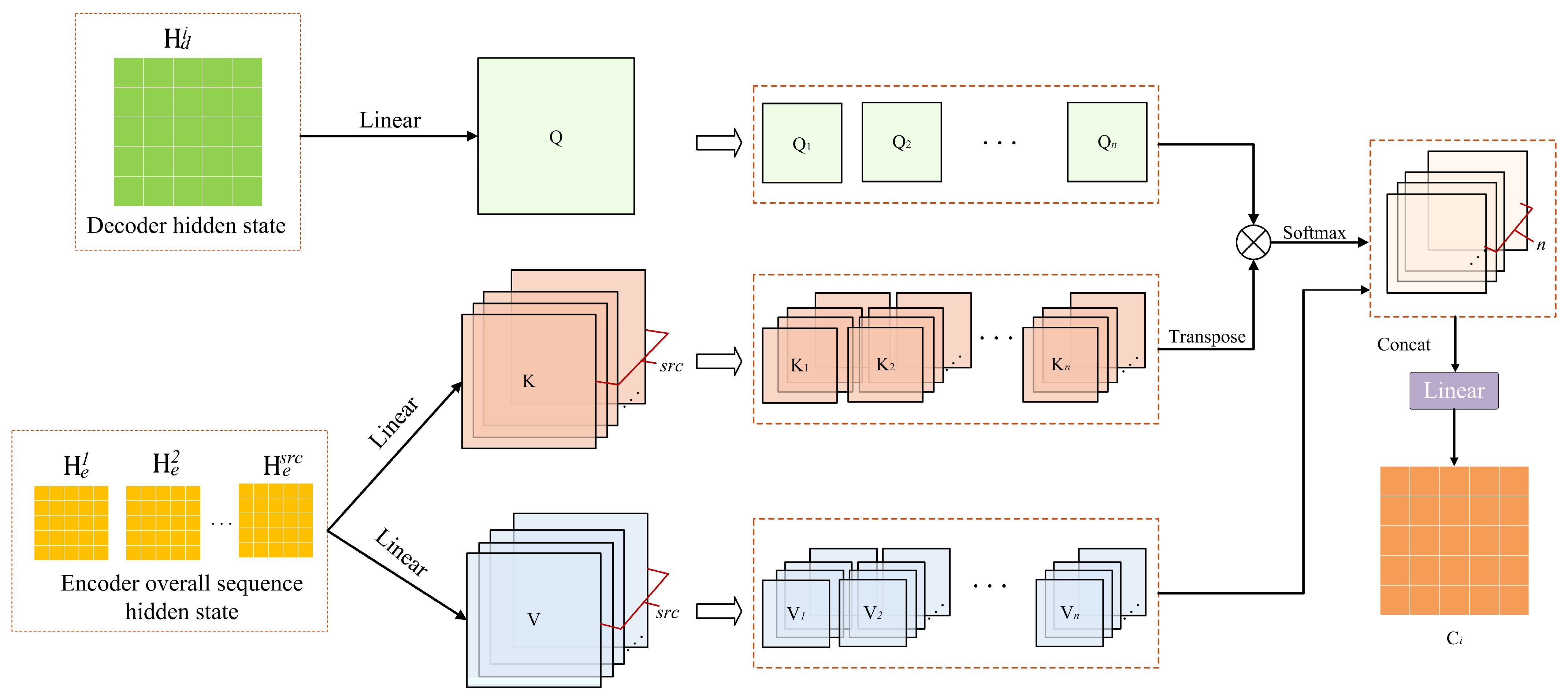
2.2. Cross-Attention Mechanism

The feature interaction process of the multi-head attention mechanism is shown in Figure 3 [17]. The input sequence passes through three linear projection layers in parallel to generate the query matrix (Q), the key matrix (K), and the value matrix (V), respectively. The query matrix (Q) is obtained by the linear mapping of the hidden state of the decoder at the corresponding time, and the key matrix (K) and the value matrix (V) are obtained by the linear mapping of the hidden state of the whole sequence of the encoder. In the dot product attention calculation stage, the similarity between elements is obtained by the matrix dot product operation of Q and K. After the scaling factor is adjusted, the SoftMax function is used for normalization to obtain the attention weight distribution that characterizes the correlation strength of different positions. Finally, the weight and the value matrix V are weighted and fused. The multi-head mechanism evenly divides the Q, K, and V matrices into n ‘attention heads’ in the feature dimension. Each subspace is calculated by independent scaling, dot product attention, to form n sets of feature representations captured in different dimensions. Each ‘head’ can independently learn the features of sequence data in each subspace. Then, the results from the multi-head are combined to focus on the hierarchical characteristics of the data from different angles and enrich the expression ability of the data. The formula for calculating the multi-head attention mechanism is as follows (9)–(14):

$${\mathrm{Q}}_{\mathrm{i}}={\mathrm{X}}_1\times {\mathrm{W}}_{\mathrm{q}\mathrm{i}}$$

(9)

$${\mathrm{K}}_{\mathrm{i}}={\mathrm{X}}_2\times {\mathrm{W}}_{\mathrm{k}\mathrm{i}}$$

(10)

$${\mathrm{V}}_{\mathrm{i}}={\mathrm{X}}_3\times {\mathrm{W}}_{\mathrm{v}\mathrm{i}}$$

(11)

$${\mathrm{A}\mathrm{t}\mathrm{t}\mathrm{e}\mathrm{n}\mathrm{t}\mathrm{i}\mathrm{o}\mathrm{n}}_{\mathrm{i}}({\mathrm{Q}}_{\mathrm{i}},{\mathrm{K}}_{\mathrm{i}},{\mathrm{V}}_{\mathrm{i}})=\mathrm{S}\mathrm{o}\mathrm{f}\mathrm{t}\mathrm{m}\mathrm{a}\mathrm{x}[{\displaystyle \frac{{\mathrm{Q}}_{\mathrm{i}}{\mathrm{K}}_{\mathrm{i}}^{\mathrm{T}}}{\sqrt{{\mathrm{d}}_{\mathrm{k}}}}}]{\mathrm{V}}_{\mathrm{i}}$$

(12)

$$\mathrm{n}(\mathrm{Q},\mathrm{K},\mathrm{V})=\mathrm{C}\mathrm{o}\mathrm{n}\mathrm{c}\mathrm{a}\mathrm{t}(h_1,h_2,\cdots h_{\mathrm{n}})$$

(13)

$$\mathrm{C}=\mathrm{n}(\mathrm{Q},\mathrm{K},\mathrm{V})\times {\mathrm{W}}_{\mathrm{o}}+{\mathrm{b}}_{\mathrm{o}}$$

(14)

where ${\mathrm{X}}_1$, ${\mathrm{X}}_2$, and ${\mathrm{X}}_3$ represent the three input sequences, respectively; i represents the index of the ith head; ${\mathrm{W}}_{\mathrm{q}\mathrm{i}}$, ${\mathrm{W}}_{\mathrm{k}\mathrm{i}}$, and ${\mathrm{W}}_{\mathrm{v}\mathrm{i}}$ represent the weight matrices for the Q, K, and V variables in the ith head, respectively; ${\mathrm{d}}_{\mathrm{k}}$ denotes the dimension of the kth key; n represents the total number of “head”; $\mathrm{C}$ represents the outputs of the attention layer.

2.3. Structure of the Proposed CGCA Model

2.3.1. Spatiotemporal Dimensions of the Model Input and Output

In the input data processing, as shown in Figure 4, the spatial dimension constructs the deflection value of the inclinometer section, the buried depth position of the monitoring point and the excavation working condition parameters at the corresponding time into a 2D image matrix: the inclinometer data and the buried depth position are mapped one by one, and the excavation working condition parameters are repeated horizontally according to the actual construction state. Expand construction parameters to full depth coverage to ensure that each burial depth position is associated with complete working condition information. The specific functions and classifications of model parameters are shown in

Table 1. Classification and function of model input parameters.

Input Category	Specific Parameters	Data Sources	Model Function
Inclinometer data	Horizontal displacement of the inclinometer tube	On-site monitoring	Capture the spatiotemporal features of deformation
Buried depth	Depth coordinates of monitoring points	Design drawing of the inclinometer tube	Correlation between structural location and deformation
Excavation conditions	Excavation depth	Construction Log	Reflect the immediate impact of construction dynamics on deformation

.

In the convolution feature extraction, the spatial correlation features of deflection at different depths are mined by a sliding window operation along the buried depth direction. The time dimension collects data at intervals of days, and the 2D images at each monitoring time are input as time series to form a spatio-temporally coupled multi-dimensional data representation system. The output data only maps the predicted values of the inclination at each buried depth, and the accurate prediction results provide a quantitative basis for engineering early warning and construction guidance.

2.3.2. CGCA Model

In this study, a CGCA model was constructed to predict the deflection of the inclined section of the retaining structure. Based on the encoder–decoder architecture, the model integrates ConvGRU to realize the hierarchical extraction of spatio-temporal features, and dynamically calculates the correlation weight of spatio-temporal data through the cross-attention mechanism to accurately model the complex spatio-temporal coupling relationship. The attention vectors generated by the cross-attention mechanism amplify spatio-temporal features corresponding to different historical moments in their temporal weight distribution: these moments exhibit variations in construction disturbances and soil states, inducing changes in soil stress paths and structural constraints—key drivers of enclosure structure deformation evolution. Higher temporal weights indicate that deformation characteristics captured in these stages have a stronger correlation with subsequent deflection trends, effectively encoding the impact of excavation on enclosure deformation. Meanwhile, their spatial weight distribution focuses on deflection trends across different measurement points of the enclosure structure at the same time, thus capturing overall deformation features (e.g., bulging shapes). By serving as key features for decoder input, these attention vectors effectively enhance the prediction accuracy of enclosure deformation.

As shown in Figure 5, the CGCA model takes the image data matrix of n days as input, corresponding to the measured section data of the next day. The model uses a two-layer ConvGRU network to achieve hierarchical extraction of spatio-temporal features: state 1 directly captures the local constraint relationship between the inclinometer data, such as the mutual limitation of deflection at different depths; state 2 extracts global morphological features based on the first layer of features, such as the overall distribution of the drum belly shape of the inclinometer curve. The hierarchical mechanism realizes multi-scale feature expression from local details to overall shape, and provides data support for accurate prediction.

2.4. Collaborative Optimization Strategy

The Adam optimizer combines the advantages of momentum optimization (Momentum) and adaptive learning rate (RMSProp), and shows significant optimization performance in geotechnical engineering tasks. However, at present, the application scenarios of deep learning models based on this optimizer are still mainly focused on data sets with stable data changes and single input features [15,23]. The soil settlement caused by vacuum preloading is a complex nonlinear process coupled with multi-source time-varying factors such as the dynamic evolution of vacuum degree, the variability of soil physical parameters, and the dissipation law of pore water pressure. Its highly dynamic and strong nonlinear characteristics put forward strict requirements on the robustness of the model and learning strategy. In this study, multi-point full-cycle construction data and long-term time-series data sets with noise interference are integrated. The design of efficient optimization strategies is not only a key path to simplify parameter tuning, improve training efficiency and optimization effect, but also a core technology to enhance the model’s cross-scene generalization ability.

Aiming at the generalized scene data set composed of multi-point full-cycle construction data, this study proposes a collaborative optimization strategy combining AdamW and Lookahead. Among them, AdamW imposes structural constraints on the parameter update process through the weight attenuation regularization mechanism independent of gradient calculation, and suppresses the overfitting of the model to the training data from the optimization mechanism level. Lookahead uses the exponential moving average strategy of fast and slow weights to dynamically smooth the optimized trajectory and effectively avoid the local optimal trap. The two form a strategic synergy through the dual mechanism of regularization constraint and optimal trajectory regulation. While ensuring the stability of the training process, the generalization performance of the model on the test set is improved, so that the model has stronger prediction adaptability and reliability for new measurement point data that are not involved in training.

The AdamW optimizer performs weight decay directly when the parameters are updated, rather than adding L2 regularization to the gradient calculation. The independent weight decay of AdamW makes weight decay a real regularization term without interfering with the gradient estimation, which makes the generalization ability of the model stronger [24]. The specific calculation process of the AdamW optimizer is as follows (15)–(17):

$${\mathrm{m}}_{\mathrm{t}}={\mathrm{\beta }}_1{\mathrm{m}}_{\mathrm{t}-1}+(1-{\mathrm{\beta }}_1){\mathrm{g}}_{\mathrm{t}}$$

(15)

$$v_t={\beta }_2{v}_{t-1}+(1-{\beta }_2)g_t^2$$

(16)

$${\theta }_{t+1}={\theta }_t-\eta {\displaystyle \frac{m_t}{\sqrt{v_t}+\epsilon }}-\eta \lambda {\theta }_t$$

(17)

where ${\mathrm{g}}_{\mathrm{t}}$ represents the update gradient of the parameter; ${\mathrm{m}}_{\mathrm{t}}$, ${\mathrm{\beta }}_1$, ${\mathrm{v}}_{\mathrm{t}}$, and ${\mathrm{\beta }}_2$ represent first-order momentum, first-order momentum coefficient, second-order momentum, and second-order momentum coefficient, respectively; $\mathrm{\eta }$ represents the learning rate; $\mathrm{\lambda }$ represents weight attenuation coefficient; $\mathrm{\epsilon }$ represents a numerical stability constant.

Lookahead optimization uses a combination of slow and fast weights to update the weight parameters [25]. It is generated by the inner loop optimizer k sequence weights; the inner loop optimizer here is the AdamW optimizer. After k weight updates, it is saved with a sequence. When the end of each round of the internal cycle, according to the k-time weight of the current round, the slow weight is calculated, which is calculated by the exponential moving average (EMA) algorithm. Specific as (18).

$${\phi }_{t+1}={\phi }_t+\alpha ({\theta }_{t,k}-{\phi }_t)=\alpha [{\theta }_{t,k}+(1-\alpha ){\theta }_{t-1,k}+\cdots {(1-\alpha )}^{t-1}{\theta }_{0,k}]+{(1-\alpha )}^t{\phi }_0$$

(18)

where ${\varphi }_{\mathrm{t}+1}$ denotes the slow weight parameter at time t + 1; $\mathrm{\alpha }$ represents the mixing coefficient and controls the influence degree of fast weight on slow weight; ${\mathrm{\theta }}_{\mathrm{t},\mathrm{k}}$ denotes the fast weight of the kth update at time t; ${\varphi }_0$ represents the initial value of the weight as the starting point of the iterative update.

The parameter used in the final model is the slow weight, so the fast weight is equivalent to performing a series of experiments, and then the slow weight selects a better direction according to the experimental results. Because the fast update may carry out more radical exploration in the parameter space, the training of the model is not stable enough, while the slow update can smooth the fluctuation caused by the fast update by a weighted average of the fast parameters, making the training of the model more stable and avoiding falling into the local optimal solution.

2.5. Flowchart of the Proposed Method

As shown in Figure 6, the overall process of the proposed framework consists of three core steps: data preparation, model construction, and performance evaluation. Firstly, the deflection value of the site retaining structure and its corresponding lateral depth and construction condition data are collected, and different features are normalized, respectively, and then spliced into a two-dimensional matrix according to the way shown in Figure 4. The training samples are generated by sliding the time window, and the data set is reconstructed according to a proportion of 80% training set and 20% test set. Based on the training set, MSE is used as the loss function to train the CGCA model, and the optimal model with the minimum loss function is iteratively searched by the combination optimization strategy of AdamW and Lookahead. Finally, the performance of the trained model is evaluated.

Three evaluation indexes, mean absolute error (MAE), root mean square error (RMSE), and coefficient of determination (R²), were used to evaluate the performance of the model, and the formulas were shown in (19)–(21).

$$\mathrm{M}\mathrm{A}\mathrm{E}={\displaystyle \frac{1}{\mathrm{n}}}{\sum }_{\mathrm{i}=1}^{\mathrm{n}}\left|{\mathrm{y}}_{\mathrm{i}}-{\widehat{\mathrm{y}}}_{\mathrm{i}}\right|$$

(19)

$$\mathrm{R}\mathrm{M}\mathrm{S}\mathrm{E}=\sqrt{{\displaystyle \frac{1}{\mathrm{n}}}{\sum }_{\mathrm{i}=1}^{\mathrm{n}}{({\mathrm{y}}_{\mathrm{i}}-{\widehat{\mathrm{y}}}_{\mathrm{i}})}^2}$$

(20)

$${\mathrm{R}}^2=1-{\displaystyle \frac{\sum {({\mathrm{y}}_{\mathrm{i}}-{\widehat{\mathrm{y}}}_{\mathrm{i}})}^2}{\sum {({\mathrm{y}}_{\mathrm{i}}-\overline{\mathrm{y}})}^2}}$$

(21)

where n is the number of predicted time points, ${\widehat{\mathrm{y}}}_{\mathrm{i}}$ is the predicted soil settlement value, ${\mathrm{y}}_{\mathrm{i}}$ is the actual soil settlement value, $\overline{\mathrm{y}}$ is the actual soil average settlement value.

3. Case Study

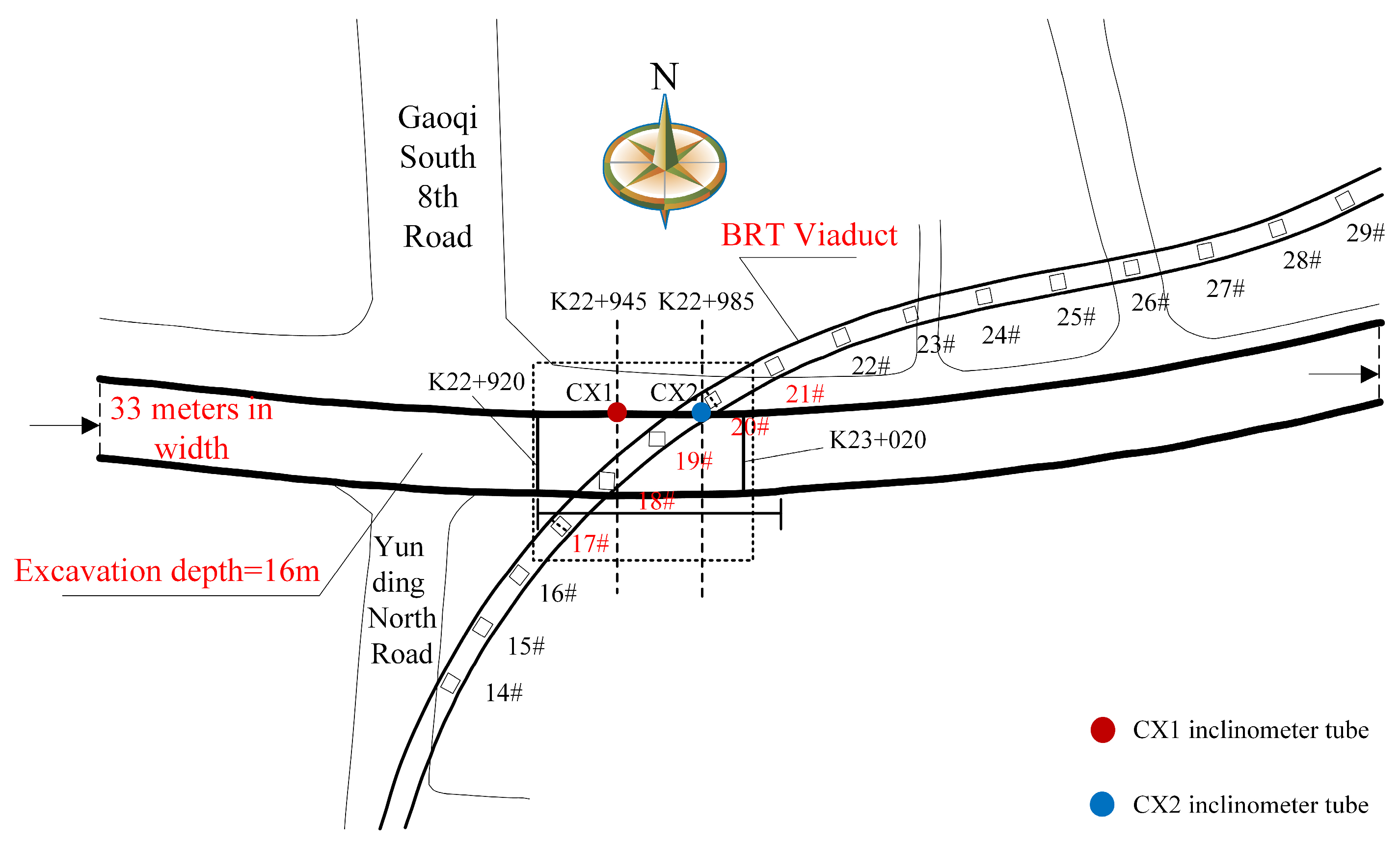
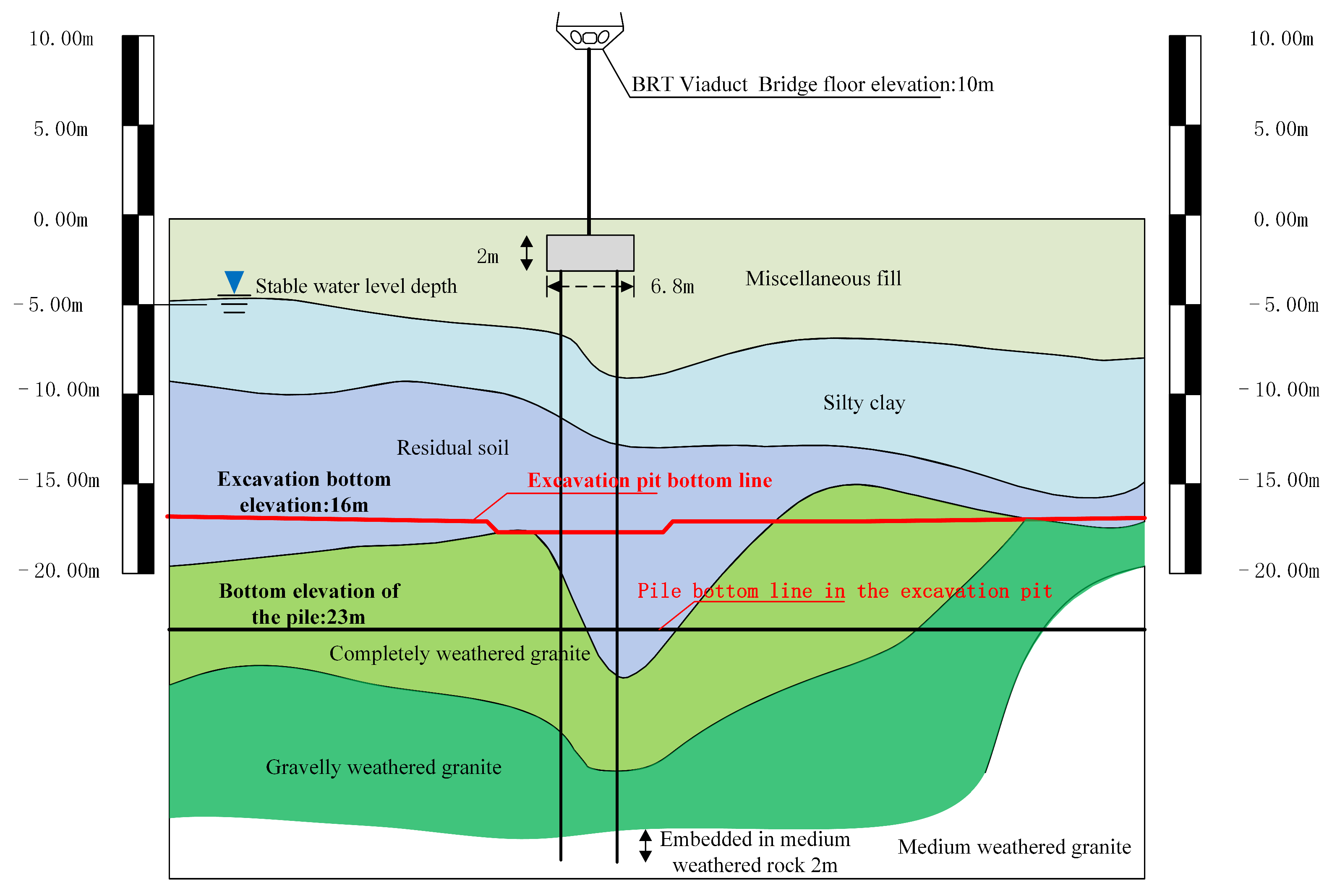
3.1. Project Overview

The main tunnel of Fangzhong Road in Xiamen Second East Passage passes through the BRT operating bridge at the intersection of Yunding North Road (K22 + 920 – K23 + 020). This special working condition puts forward extremely high requirements for the structural stability during the excavation of the foundation pit, so this area is selected as the test and verification project of the proposed model. As shown in Figure 7, the excavation depth of the foundation pit in this section is 16 m, and the width is about 33 m. The composite support system of ‘Φ1000 @ 1200 bored pile + Φ800 @ 45 high-pressure jet grouting pile waterproof curtain + internal support’ is adopted, and a single row of vertical column piles is set in the middle of the foundation pit to enhance the overall stability. The supporting structure is specifically arranged as an 800 × 800 mm concrete support and two steel pipe supports. The transverse spacing of the concrete support is about 8 m, and the transverse spacing of the steel support is encrypted to 4 m, so as to ensure the safety and stability of the upper operating bridge.

Figure 8 shows the distribution of soil in the geological distribution section (K22 + 865–K23 + 065), the soil above the foundation pit bottom shows distinct layered characteristics: The surface miscellaneous fill is continuously distributed, with an average thickness of about 4.24 m, piled for more than 5 years, featuring poor compactness and uniformity, and low mechanical strength. The middle silty clay, with a thickness of 1.0–5.2 m, is a soft soil with high water content and compressibility, low shear strength, and strong thixotropy and rheology. The lower residual soil has an average thickness of about 4.89 m, with high original structural strength but a sharp decrease after disturbance, and is prone to softening and disintegration when immersed in water. Among the weathered granite below the pit bottom, the completely weathered and gravelly weathered ones are prone to softening and disintegration when encountering water, with poor self-stability; the moderately weathered one has undeveloped joints and fissures, good integrity, high strength and bearing capacity, and are an excellent foundation bearing layer.

3.2. Data Acquisition

In this study, the CX1 inclinometer tube of K22 + 945 section and the CX2 inclinometer tube of K22 + 985 section were selected to construct data set 1 and data set 2, respectively. Among them, the depth of the CX1 inclinometer tube is 20.5 m, and 41 monitoring points are set at intervals of 0.5 m. The depth of the CX2 inclinometer tube is 19.5 m, with a total of 39 monitoring points, also arranged at a distance of 0.5 m. The monitoring period of the data set is selected from 28 October 2021 to 12 January 2022 during the excavation of the foundation pit. It is mainly based on two considerations: one is that the initial value of manual monitoring is not collected at the initial stage of the excavation of the foundation pit, and the other is that the retaining structure tends to be stable after the construction of the foundation pit floor is completed. The deformation data is of little significance to the research, so the data from the above stages are not included in the research scope. The specific excavation method of the foundation pit is detailed in

Table 2. Construction stages.

Phase	Project Profile	Construction Time	Period/Day
1	Sloped excavation was conducted to a depth of −2.5 m, followed by casting the first layer of concrete support.	13 October 2021~30 October 2021	17
2	Excavate to −7 m in turn, and set up the second steel support.	30 October 2021~20 November 2021	21
3	Excavate to −12 m, and set up the third steel support.	20 November 2021~16 December 2021	26
4	Excavating to the bottom of the pit −16 m.	16 December 2021~26 December 2021	10
5	The cushion is applied, and the bottom plate is poured.	26 December 2021~13 January 2022	18

.

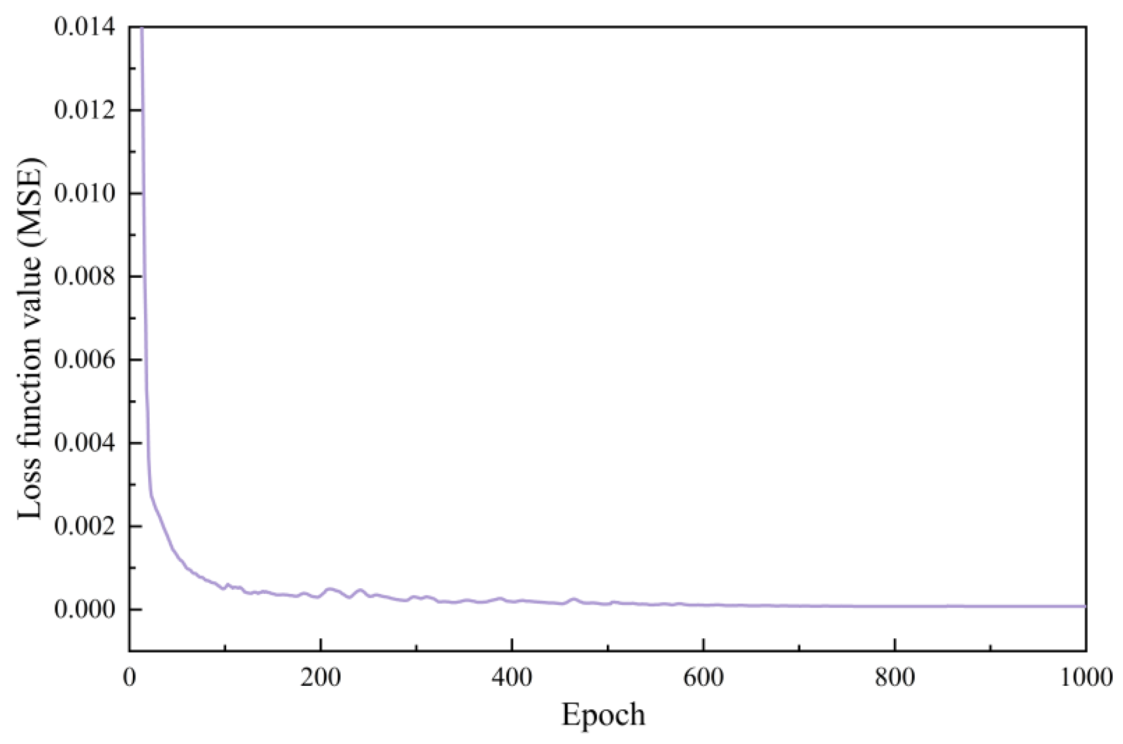
4. Construction of CGCA Model

The performance of the model is greatly affected by hyperparameters, including the hidden layer dimension, batch size, and learning rate in the model. As shown in

Table 3. Model hyperparameters.

Symbol	Meaning Description	Specification
${\mathrm{d}}_{\mathrm{e}\mathrm{n}\mathrm{c}}$	Encoder hidden layer dimension	256
${\mathrm{d}}_{\mathrm{d}\mathrm{e}\mathrm{c}}$	Decoder hidden layer dimension	256
${\mathrm{n}}_{\mathrm{e}\mathrm{n}\mathrm{c}}$	Encoder neural network layers	2
${\mathrm{n}}_{\mathrm{d}\mathrm{e}\mathrm{c}}$	Decoder neural network layers	2
src	Encoder length	5
trg	Decoder length	1
Batch size	The size of a training sample	4
${\mathrm{\beta }}_1$	The first-order momentum coefficient	0.9
${\mathrm{\beta }}_2$	Second-order momentum coefficient	0.99
$\mathrm{\lambda }$	Weight attenuation coefficient	0.001
$\mathrm{k}$	Parameter update interval	10
$\mathrm{\alpha }$	Weighting coefficient of historical parameters	0.5
$\mathrm{T}$	The maximum number of training iteration rounds	1000

, the encoder and decoder hidden layer dimensions are set to 256 neural units. The number of encoder neural networks is two layers, and the number of decoder layers is two layers. The encoder length of the model is set to five steps, and the decoder length is set to one step. The batch size is set to four. The optimizer adopts the combination optimization method of the AdamW basic optimizer, combined with Lookahead. Among them, the AdamW basic optimizer has a first-order momentum coefficient ${\mathrm{\beta }}_1$ of 0.9, a second-order momentum coefficient ${\mathrm{\beta }}_2$ of 0.99, and a weight attenuation coefficient $\mathrm{\lambda }$ of 0.001. In the Lookahead optimization strategy, k is set to 10, that is, every ten fast updates trigger a slow update, and the weighting coefficient α is 0.5. The maximum number of training iterations $\mathrm{T}$ is 1000.

In order to expect the stable and fast convergence of the model, a single-cycle cosine annealing method is used to reduce the learning rate ${\mathrm{\eta }}_{\mathrm{t}}$ in a cosine decreasing manner with the increase in the number of iterations. The initial learning rate ${\mathrm{\eta }}_0$ is $1\times {10}^{-4}$, and the end learning rate ${\mathrm{\eta }}_{\mathrm{T}}$ is $1\times {10}^{-6}$. It is hoped that the model will converge rapidly due to the high learning rate in the initial stage, and the loss of the model will be minimized due to the low learning rate in the middle and later stages, so as to find the optimal model. The learning rate in the training process is shown in (22).

$${\mathrm{\eta }}_{\mathrm{t}}={\mathrm{\eta }}_0+{\displaystyle \frac{1}{2}}({\mathrm{\eta }}_{\mathrm{T}}-{\mathrm{\eta }}_0)(1+\cos ({\displaystyle \frac{\mathrm{t}\mathrm{\pi }}{\mathrm{T}}}))$$

(22)

where ${\mathrm{\eta }}_{\mathrm{t}}$ is the current round of learning rate, ${\mathrm{\eta }}_0$ is the initial learning rate, ${\mathrm{\eta }}_{\mathrm{T}}$ is he end learning rate, $\mathrm{t}$ is the current number of iterations, and $\mathrm{T}$ is the maximum number of iterations.

In the process of model training and testing, this study is based on the Python (version 3.9.13) language and relies on the PyTorch (version 2.0.0+cu118) deep learning framework to complete the algorithm construction and implementation. In terms of hardware configuration, Intel (R) Xeon (R) Gold 6130 CPU (32 core, 2.10 GHz) and NVIDIA GeForce RTX 3090 GPU are used to provide powerful computing support for model training and testing, and ensure the efficient operation of deep learning tasks.

It can be seen in Figure 9 that, under the condition that the encoder length is 5 and the decoder length is 1, the model training process constructed by the CX1 inclinometer data set takes about 1427.19 s. At the beginning of the iteration, the loss function value decreases rapidly. With the gradual advancement of training rounds, the loss is continuously optimized at a steady rate. Until the 1000th round of training, the loss value tends to be stable, and the model achieves a higher degree of convergence. The whole training process clearly shows a good training dynamic from fast error attenuation to stable convergence, which fully verifies the effectiveness and stability of the model optimization process.

5. Results

5.1. Performance of CGCA

In this study, the model was constructed using a configuration with an encoder length of 5 and a decoder length of 1. Considering the characteristics of the excavation process of the whole foundation pit project, all the data are arranged in chronological order, and the first 80% of the data (a total of 57 samples) are divided into training sets for model training. The last 20% of the data (a total of 15 samples) is used as a test set to verify the model effect. Such a division method can not only make the model fully learn the main characteristics and changing rules in the process of foundation pit excavation, but also effectively evaluate the generalization ability of the model, so as to ensure that the model has good prediction performance in practical applications.

Figure 10 and Figure 11 show the comparison of the prediction results of the CGCA model under different data set tests. It can be clearly observed from the diagram that the predicted surface of the CGCA model is similar to the height of the surface formed by the actual working condition monitoring data. The predicted results not only show the bulging shape deformation consistent with the actual measurement, but also the overall shape change is continuous and smooth, which fully demonstrates the model’s strong ability to capture spatial features. This accurate spatial shape fitting is an intuitive manifestation of the model’s extremely high prediction accuracy. The quantitative performance indicators further consolidate this conclusion: in the test of data set 1, the root mean square error (RMSE) of the model is 0.385 mm, the mean absolute error (MAE) is 0.314 mm, and the coefficient of determination R² is as high as 0.9960; the test results of data set 2 are also excellent, RMSE is 0.439 mm, MAE is 0.359 mm, and R² is 0.9942. These data clearly show that the CGCA model has both strong prediction performance and high reliability in the prediction task.

As shown in Figure 12 and Figure 13, the measured-predicted scatter plots of data set 1 (CX1 inclinometer) and data set 2 (CX2 inclinometer) show that the CGCA model exhibits excellent performance under different data sets. The scatter points of the two maps are closely distributed along the y = x baseline, and the determination coefficient R² exceeds 0.99 (CX1 is 0.996, CX2 is 0.994), which fully proves that the model can accurately capture the spatio-temporal nonlinear characteristics of the deformation of the envelope structure and has high robustness. However, the model has differences in scene adaptability: the scatter distribution of the CX1 inclinometer is more balanced. When the lateral displacement value is large, the prediction result is slightly larger; while the lateral displacement value is small, the prediction result is highly consistent with the measured value. The monitoring data of the CX2 inclinometer tube shows a trend of being larger than the predicted data. Further analysis of the reasons shows that the excavation project where the CX1 inclinometer tube is located belongs to the standard section, which is less affected by the external construction and related loads, and the data change characteristics are relatively stable. The CX2 inclinometer tube is adjacent to the 20 # bridge structure. The dynamic load of the bridge deck, the interaction between the soil stress release and the bridge structure during the excavation process, and other factors significantly enhance the influence of the construction dynamic load, and the nonlinear characteristics of the data are more prominent.

Although the CX1 and CX2 sections have significant geological undulations, the deformation prediction of the enclosure structure at this section shows robust performance. This indicates the adaptability of the CGCA model to different soil conditions, even in different soil types and huge geological undulations, and it can effectively capture the nonlinear deformation characteristics of enclosure structures. For different types of supports, the model was tested under a composite support system (drilled pile + steel pillar); Its adaptability to other types of support, such as soil nail support and underground continuous walls, still needs to be verified, as different support stiffness and deformation mechanisms may alter the spatiotemporal correlations that the model relies on.

5.2. The Effect of Encoder Length on Model Performance

As shown in Figure 14, in the test set prediction task of the CGCA model for the deformation of the envelope structure, data set 1 is used for model training and testing, and there is a significant correlation between the length of the model encoder (i.e., the length of the input sequence) and the performance. From the perspective of index performance: the mean absolute error (MAE) and root mean square error (RMSE) show a trend of ‘first decrease and then increase’ with the increase in length, and reach their lowest when the input is 5 days, and the subsequent length increases, and the error index reverses. The coefficient of determination (R²) reached a peak when the length increased to 5 days, and then decreased significantly with the increase in length. This law reveals that moderately extending the input sequence can help the model to better capture the dynamic deformation characteristics of the envelope structure and effectively improve the prediction accuracy and fitting effect. However, if the sequence is too long, it will cause feature redundancy, increase the learning burden of the model, and reduce the prediction accuracy and overall fitting ability. It can be seen that there is an optimal interval for the length of the input sequence, which needs to be reasonably regulated to balance the performance of the model and lay a solid foundation for the accurate prediction of the deformation of the retaining structure.

5.3. Comparative Experiment

In this study, under the sequence prediction framework with an encoder length of 5 and a decoder length of 1, data set 1 is used for model training and testing. Through three performance indicators of MAE, MSE, and R, the original CGCA model and the CGCA model using the Adam optimizer version are systematically compared. The CGCA model that eliminates the multi-head attention mechanism, and the GRU baseline model with parameter isomorphism and combined optimization strategy, verify the advantages of each architecture design in the CGCA model and the superior performance compared with other models.

Table 4. Comparison table of the whole process prediction performance index of each model.

Model	MAE	RMSE	R2
CGCA	0.31	0.39	0.996
REMOVE_ATTENTION	0.53	0.63	0.989
ADAM	0.90	1.14	0.966
GRU	0.60	0.72	0.986

shows the evaluation indexes MAE, RMSE, and R² of each comparison model under the whole test set. Based on the comparative analysis of the experimental data, the CGCA model shows significant advantages in the deformation prediction of the envelope structure: it leads with the optimal MAE (0.31 mm), RMSE (0.39 mm) and near-perfect R² (0.996), indicating that the model can accurately capture the spatial and temporal deformation characteristics of the envelope structure. After removing the multi-head attention mechanism, the performance of the model decreases, which verifies the key role of the mechanism in long-term dependence modeling through step-length feature fusion. The comparison of optimizers shows that there are serious adaptation problems in the ADAM series, and the combination optimization strategy of ADAMW combined with LOOKAHEAD is robust and has good performance, which highlights the effectiveness of the model combination optimization strategy. The results show that the CGCA model achieves excellent prediction accuracy in the deformation prediction of envelope structure through the collaborative design of an attention mechanism and a combinatorial optimization strategy.

The Taylor plot integrates three indicators: correlation coefficient (R), standard deviation (SD), and central root mean square error (CRMSD), as shown in Equations (23)–(25). R and SD are used to quantify the comparability between predicted and actual values, and CRMSD is used to describe the deviation between predicted and actual values. If the CRMSD and R values are close to 0 and 1, respectively, it indicates that the model has excellent performance. If the position of the model in the Taylor diagram is close to the center of the yellow arc, the standard deviation between the predicted value and the actual value is similar. In the Taylor diagram, the blue line depicts the contour of the correlation coefficient and measures the linear correlation between the predicted and real data. The gray arc is the contour of the standard deviation, which measures the dispersion degree of data. The orange arc represents the contour of the center root mean square error and measures the overall deviation between the predicted data and the real data.

$$\mathrm{R}={\displaystyle \frac{\left[{\sum }_{\mathrm{i}=1}^{\mathrm{n}}({\widehat{\mathrm{y}}}_{\mathrm{i}}-\overline{\widehat{y}})\times ({\mathrm{y}}_{\mathrm{i}}-\overline{y})\right]}{\sqrt{{\sum }_{\mathrm{i}=1}^{\mathrm{n}}{({\widehat{\mathrm{y}}}_{\mathrm{i}}-\overline{\widehat{y}})}^2\times {({\mathrm{y}}_{\mathrm{i}}-\overline{y})}^2}}}$$

(23)

$${\mathrm{S}\mathrm{D}}_{\mathrm{f}}=\sqrt{{\displaystyle \frac{1}{\mathrm{n}}}{\sum }_{\mathrm{i}=1}^{\mathrm{n}}{({\widehat{\mathrm{y}}}_{\mathrm{i}}-\overline{\widehat{\mathrm{y}}})}^2}, {\mathrm{S}\mathrm{D}}_{\mathrm{r}}=\sqrt{{\displaystyle \frac{1}{\mathrm{n}}}{\sum }_{\mathrm{i}=1}^{\mathrm{n}}{\left({\mathrm{y}}_{\mathrm{i}}-\overline{y}\right)}^2}$$

(24)

$$\mathrm{C}\mathrm{R}\mathrm{M}\mathrm{S}\mathrm{D}=\sqrt{{\displaystyle \frac{1}{\mathrm{n}}}{\sum }_{\mathrm{i}=1}^{\mathrm{n}}{[({\widehat{\mathrm{y}}}_{\mathrm{i}}-\overline{\widehat{\mathrm{y}}})}^2-{\left({\mathrm{y}}_{\mathrm{i}}-\overline{y}\right)}^2]}$$

(25)

where ${\widehat{\mathrm{y}}}_{\mathrm{i}}$ is the average value of the model prediction value, ${\mathrm{y}}_{\mathrm{i}}$ the actual measurement value, $\overline{\widehat{\mathrm{y}}}$ is the average value of the model prediction value, ${\mathrm{S}\mathrm{D}}_{\mathrm{f}}$ is the standard deviation of the model predictive value, ${\mathrm{S}\mathrm{D}}_{\mathrm{r}}$ is the standard deviation of the actual measured value, and n is the total number of sample data points.

As shown in Figure 15, the Taylor diagram comprehensively compares the prediction performance of different models under the full test set: the dispersion difference between the model based on the ADAM optimizer and the measured data is significant, and the correlation is low, especially in the scenario where the data changes drastically. It is difficult to accurately capture the characteristics of data fluctuations; the ADAM + LOOKAHEAD combination strategy model effectively reduces the loss function value by optimizing the weight update mechanism, significantly reduces the fluctuation difference between the predicted value and the measured value, and the overall performance is significantly better than the single ADAM optimization strategy. In contrast, although the standard deviation of the GRU model with the same parameter scale is close to the real data, its correlation with the measured data is obviously insufficient, indicating that the model is weaker than the CGCA model in terms of spatio-temporal feature capture ability and prediction accuracy. In addition, the introduction of the cross-attention mechanism further verifies its positive effect on improving the spatio-temporal feature extraction ability and prediction performance of the model.

6. Conclusions

In this study, a deep learning prediction model (CGCA) based on an encoder–decoder architecture, convolutional gated recurrent unit (ConvGRU), and a cross-attention mechanism is proposed to achieve accurate prediction of envelope deformation. The model deeply integrates multi-dimensional information such as inclinometer monitoring data, construction conditions, and buried depth, and uses AdamW and Lookahead combination optimization strategy to improve training effect and generalization ability. The main conclusions are as follows:

(1)

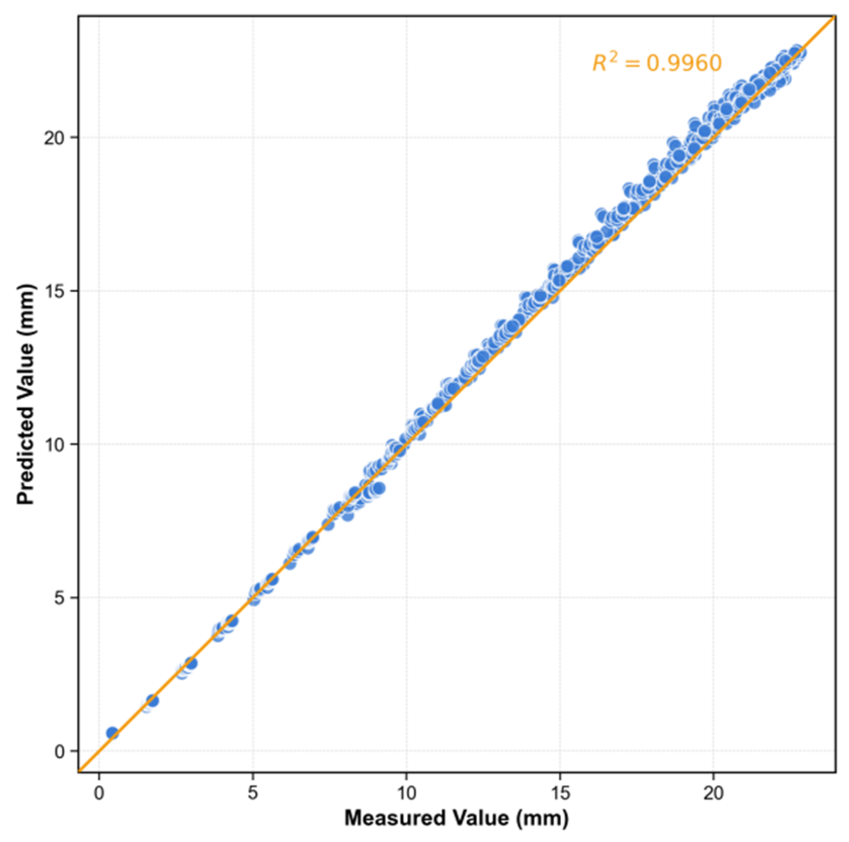
Based on the measured data from the deep foundation pit project of the open-cut underpass for elevated bridges along Xiamen’s Second East Passage, the CGCA model demonstrated excellent prediction accuracy on the test set: with a root mean square error (RMSE) of 0.385 mm, a mean absolute error (MAE) of 0.314 mm, and a coefficient of determination (R²) of 0.996. This confirms the model’s strong capability to capture the spatiotemporal deformation characteristics of retaining structures, providing technical support for “millimeter-level early warning + dynamic decision-making” in high-risk foundation pit projects within densely populated urban areas.

(2)

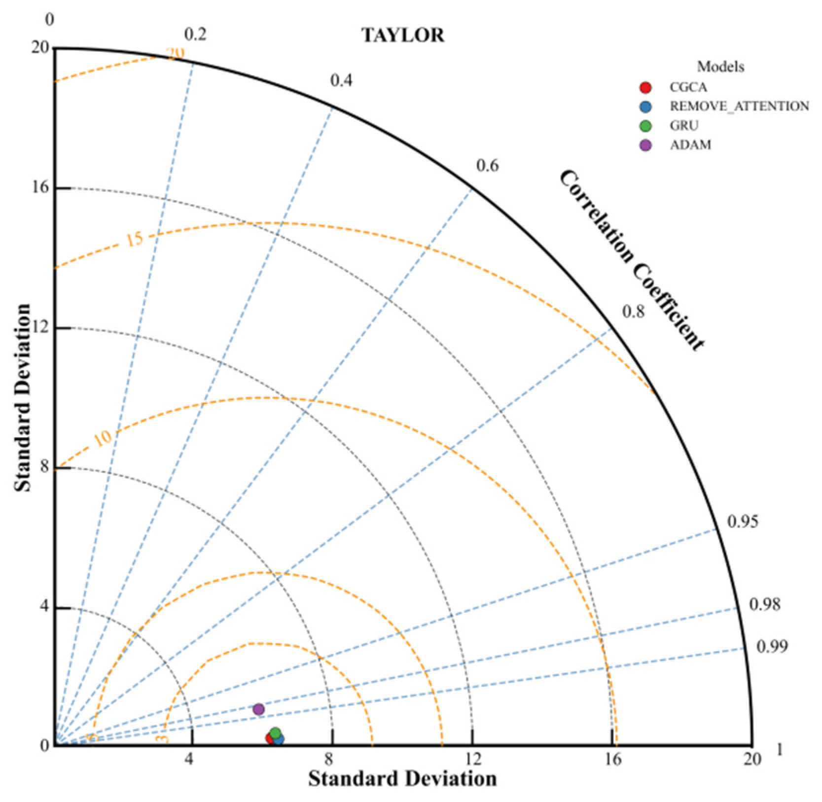
Effectiveness of architecture design and optimization strategy: Comparative experiments show that the performance of the CGCA model is significantly better than other benchmark models. After eliminating the cross-attention mechanism, the performance of the model decreased (MAE increased to 0.53 mm, R² decreased to 0.989), which verified the key role of the mechanism in long-term dependence modeling through step-length feature fusion. The combined optimization strategy of AdamW and Lookahead reduces the prediction error by 54% compared with the single Adam optimizer, highlighting the advantages of the weight update mechanism in suppressing overfitting and improving generalization. Compared with the GRU model with parameter isomorphism, the CGCA model shows higher correlation and lower dispersion, which confirms its superiority in spatio-temporal feature extraction.

(3)

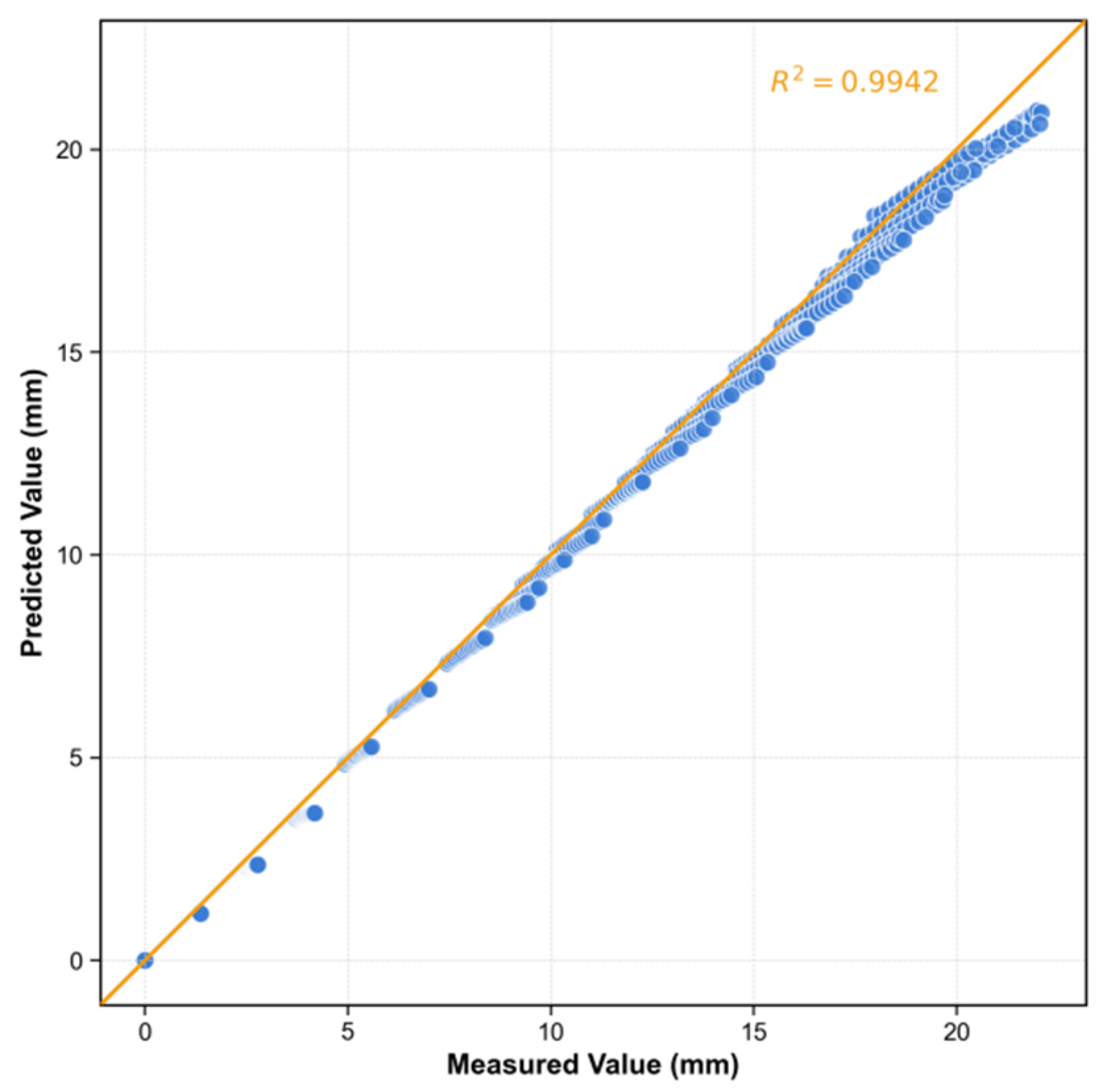
The model shows excellent performance under different data sets, and still maintains high robustness under dynamic interference conditions (such as the CX2 section adjacent to the BRT bridge): Although the data nonlinearity is enhanced by the coupling of traffic dynamic load and soil-structure interaction, the model still maintains a high-precision prediction of MAE < 0.36 mm through multi-dimensional information fusion (burial depth, working condition) and attention weighting mechanism, which fully verifies its universality and robustness in complex engineering environments.

References

1. Huang, J.; Liu, J.; Guo, K.; Wu, C.; Yang, S.; Luo, M.; Lu, Y. Numerical Simulation Study on the Impact of Deep Foundation Pit Excavation on Adjacent Rail Transit Structures—A Case Study. Buildings 2024, 14, 1853. [Google Scholar] [CrossRef]
2. Xu, Q.; Xie, J.; Lu, L.; Wang, Y.; Wu, C.; Meng, Q. Numerical and Theoretical Analysis on Soil Arching Effect of Prefabricated Piles as Deep Foundation Pit Supports. Undergr. Space 2024, 16, 314–330. [Google Scholar] [CrossRef]
3. Cheng, K.; Riqing, X.; Ying, H.; Cungang, L.; Gan, X. Simplified Method for Calculating Ground Lateral Displacement Induced by Foundation Pit Excavation. Eng. Comput. 2020, 37, 2501–2516. [Google Scholar] [CrossRef]
4. Zhu, Y.; Wang, W.; Xu, Z.; Chen, J.; Zhang, J. Hydro-Mechanical Numerical Analysis of a Double-Wall Deep Excavation in a Multi-Aquifer Strata Considering Soil–Structure Interaction. Buildings 2025, 15, 989. [Google Scholar] [CrossRef]
5. Han, G.; Zhang, Y.; Zhang, J.; Zhang, H. Numerical Analysis and Optimization of Displacement of Enclosure Structure Based on MIDAS Finite Element Simulation Software. Buildings 2025, 15, 1462. [Google Scholar] [CrossRef]
6. Hong, C.; Luo, G.; Chen, W. Safety Analysis of a Deep Foundation Ditch Using Deep Learning Methods. Gondwana Res. 2023, 123, 16–26. [Google Scholar] [CrossRef]
7. Hu, H.; Hu, X.; Gong, X. Predicting the Strut Forces of the Steel Supporting Structure of Deep Excavation Considering Various Factors by Machine Learning Methods. Undergr. Space 2024, 18, 114–129. [Google Scholar] [CrossRef]
8. Wang, X.; Pan, Y.; Chen, J.; Li, M. A Spatiotemporal Feature Fusion-Based Deep Learning Framework for Synchronous Prediction of Excavation Stability. Tunn. Undergr. Space Technol. 2024, 147, 105733. [Google Scholar] [CrossRef]
9. Zhou, X.; Pan, Y.; Qin, J.; Chen, J.-J.; Gardoni, P. Spatio-Temporal Prediction of Deep Excavation-Induced Ground Settlement: A Hybrid Graphical Network Approach Considering Causality. Tunn. Undergr. Space Technol. 2024, 146, 105605. [Google Scholar] [CrossRef]
10. Deng, Z.; Xu, L.; Su, Q.; He, Y.; Li, Y. A Novel Method for Subgrade Cumulative Deformation Prediction of High-Speed Railways Based on Empiricism-Constrained Neural Network and SHapley Additive exPlanations Analysis. Transp. Geotech. 2024, 49, 101438. [Google Scholar] [CrossRef]
11. Fayaz, J.; Medalla, M.; Torres-Rodas, P.; Galasso, C. A Recurrent-Neural-Network-Based Generalized Ground-Motion Model for the Chilean Subduction Seismic Environment. Struct. Saf. 2023, 100, 102282. [Google Scholar] [CrossRef]
12. Yang, J.; Liu, Y.; Yagiz, S.; Laouafa, F. An Intelligent Procedure for Updating Deformation Prediction of Braced Excavation in Clay Using Gated Recurrent Unit Neural Networks. J. Rock Mech. Geotech. Eng. 2021, 13, 1485–1499. [Google Scholar] [CrossRef]
13. Hong, S.; Ko, S.J.; Woo, S.I.; Kwak, T.Y.; Kim, S.R. Time-Series Forecasting of Consolidation Settlement Using LSTM Network. Appl. Intell. 2024, 54, 1386–1404. [Google Scholar] [CrossRef]
14. Yang, B.; Yin, K.; Lacasse, S.; Liu, Z. Time Series Analysis and Long Short-Term Memory Neural Network to Predict Landslide Displacement. Landslides 2019, 16, 677–694. [Google Scholar] [CrossRef]
15. Zhang, W.S.; Yuan, Y.; Long, M.; Yao, R.H.; Jia, L.; Liu, M. Prediction of Surface Settlement around Subway Foundation Pits Based on Spatiotemporal Characteristics and Deep Learning Models. Comput. Geotech. 2024, 168, 106149. [Google Scholar] [CrossRef]
16. Jin, J.; Jin, Q.; Chen, J.; Wang, C.; Li, M.; Yu, L. Prediction of the Tunnelling Advance Speed of a Super-Large-Diameter Shield Machine Based on a KF-CNN-BiGRU Hybrid Neural Network. Measurement 2024, 230, 114517. [Google Scholar] [CrossRef]
17. Vaswani, A.; Shazeer, N.; Parmar, N.; Uszkoreit, J.; Jones, L.; Gomez, A.N.; Kaiser, L.; Polosukhin, I. Attention Is All You Need. arXiv 2017, arXiv:1706.03762. [Google Scholar]
18. Yuan, Y.; Lin, L.; Huo, L.-Z.; Kong, Y.-L.; Zhou, Z.-G.; Wu, B.; Jia, Y. Using an Attention-Based LSTM Encoder–Decoder Network for near Real-Time Disturbance Detection. IEEE J. Sel. Top. Appl. Earth Obs. Remote Sens. 2020, 13, 1819–1832. [Google Scholar] [CrossRef]
19. Zhang, W.; Zhang, P.; Yu, Y.; Li, X.; Biancardo, S.A.; Zhang, J. Missing Data Repairs for Traffic Flow with Self-Attention Generative Adversarial Imputation Net. IEEE Trans. Intell. Transp. Syst. 2022, 23, 7919–7930. [Google Scholar] [CrossRef]
20. Yang, M.; Song, M.; Guo, Y.; Lyv, Z.; Chen, W.; Yao, G. Prediction of Shield Tunneling-Induced Ground Settlement Using LSTM Architecture Enhanced by Multi-Head Self-Attention Mechanism. Tunn. Undergr. Space Technol. 2025, 161, 106536. [Google Scholar] [CrossRef]
21. Fan, G.; He, Z.; Li, J. Structural Dynamic Response Reconstruction Using Self-Attention Enhanced Generative Adversarial Networks. Eng. Struct. 2023, 276, 115334. [Google Scholar] [CrossRef]
22. Lecun, Y.; Bottou, L.; Bengio, Y.; Haffner, P. Gradient-Based Learning Applied to Document Recognition. Proc. IEEE 1998, 86, 2278–2324. [Google Scholar] [CrossRef]
23. Tao, Y.; Zeng, S.; Sun, H.; Cai, Y.; Zhang, J.; Pan, X. A Spatiotemporal Deep Learning Method for Excavation-Induced Wall Deflections. J. Rock Mech. Geotech. Eng. 2024, 16, 3327–3338. [Google Scholar] [CrossRef]
24. Loshchilov, I.; Hutter, F. Decoupled Weight Decay Regularization. arXiv 2017, arXiv:1711.05101. [Google Scholar]
25. Zhang, M.R.; Lucas, J.; Hinton, G.; Ba, J. Lookahead Optimizer: K Steps Forward, 1 Step Back. arXiv 2019, arXiv:1907.08610. [Google Scholar]
Figure 1. GRU structure.
Buildings 15 02537 g001
Figure 2. ConvGRU structure.
Buildings 15 02537 g002
Figure 3. Cross-attention mechanism operation.
Buildings 15 02537 g003
Figure 4. Spatial input features.
Buildings 15 02537 g004
Figure 5. CGCA model architecture.
Buildings 15 02537 g005
Figure 6. Flowchart of CGCA.
Buildings 15 02537 g006
Figure 7. Layout plan of the excavation project.
Buildings 15 02537 g007
Figure 8. Distribution of geological longitudinal sections.
Buildings 15 02537 g008
Figure 9. The loss function of the training model.
Buildings 15 02537 g009
Figure 10. The prediction results of the CGCA model in data set 1.
Buildings 15 02537 g010
Figure 11. The prediction results of the CGCA model in data set 2.
Buildings 15 02537 g011
Figure 12. Scatter plot of actual and predicted results in data set 1.
Buildings 15 02537 g012
Figure 13. Scatter plot of actual and predicted results in data set 2.
Buildings 15 02537 g013
Figure 14. The impact of encoder length on model performance.
Buildings 15 02537 g014
Figure 15. Comparison of multi-models based on the Taylor diagram.
Buildings 15 02537 g015