Wind-Induced Dynamic Critical Response in Buildings Using Machine Learning Techniques

Abstract

Wind is one of the main factors causing variable actions in tall buildings, and its effects cannot be neglected in the evaluation of either displacements and accelerations that develop in the structure or the internal forces generated indirectly within. However, the structural analyses necessary for these evaluations usually lead to high computational efforts, so surrogate models have been increasingly used to reduce the computational time required. In this work, five machine learning techniques are evaluated for predicting maximum displacement in buildings under dynamic wind loads: k-nearest neighbors (kNN), random forest (RF), support vector regression (SVR), Gaussian process regression (GPR), and artificial neural network (ANN). An initial dataset with 500 random samples was used to evaluate the responses generated by the models. The predictor variables were the building’s height, width, and length; average density; damping ratio; wind velocity; and ground roughness. The obtained results demonstrate that the techniques can predict dynamic responses, mainly the GPR and the ANN.

1. Introduction

Whether due to the increase in demand for space due to population growth or technological advances in materials and construction systems, the construction of increasingly taller buildings has become common. According to the Council for Tall Buildings and Urban Habitat (CTBUH), the number of tall buildings has shown an increasing trend, especially since the 2000s and in countries like China and Brazil, a BRICS country [1]. In these structures, wind load is one of the main factors causing variable actions. In the analysis of the ultimate limit states in terms of internal forces [2,3] and the analysis of serviceability limit states in terms of displacements and accelerations, effects that can cause great discomfort to users must be carefully considered [4,5]. Detailed dynamic analysis involves infinite degrees of freedom (DoFs); however, structural systems can be represented through discrete models with a finite number of DoFs, in which stiffness, mass, and damping are evaluated. Even when the system’s behavior is linear and the dynamic parameters are known, the system can be represented by a single degree of freedom (SDoF) [6,7,8]. For simpler dynamic actions, such as harmonic loads or impulse loads, closed analytical solutions can be developed; however, for random actions such as wind, it is necessary to carry out numerical analyses [9]. The analysis of free vibrations results in an eigenvalue problem in which the eigenvalues and eigenvectors give the vibration frequencies and corresponding mode shapes, respectively. Frequencies and damping ratios are important in dynamic systems because they can significantly influence the structural response. As the excitation frequency approaches the vibration frequency of the structure, the ratio between the responses obtained in dynamic and static analyses increases [10,11].

Damping can occur due to internal friction of the elements that make up the system, or between the system and the external environment, such as aerodynamic and hydrodynamic damping. Generally, damping is proportional to velocity and is expressed as a ratio ζ of critical damping, for which higher values reflect smaller response amplitudes [12,13,14]. Cruz and Miranda [15] evaluated the damping ratio experimentally in 24 buildings with heights between 28 m and 218 m when excited by natural seismic events, identifying damping ratios lower than 1.0% in some cases. Dai et al. [16] evaluated the damping ratio in reinforced concrete structures based on seismic events and associated the damping with the peak acceleration of the ground; their study identified values between 0 and 10% for damping and that for accelerations lower than 0.1 g; the data approximate the Gamma distribution. Lago et al. [17] pointed out some considerations for damping such as a lower limit equal to 0.3%, large dispersion in values especially in lower buildings, and a tendency towards lower values for greater building heights.

In general, the higher the height of the building, the lower the vibration frequencies, and for this reason, they become more susceptible to large amplitude vibrations when subjected to low-frequency dynamic actions such as wind, making dynamic analyses essential [18,19,20]. However, it is worth highlighting that even in lower structures, problems often occur due to wind action, such as roof collapses and other localized damages [21,22,23].

Regarding structural modeling, it is possible to use high- and low-fidelity models to discretize the structure and loads. For example, Vital et al. [24] created a high-fidelity 3D digital model of bridges integrating Terrestrial Laser Scanning and photogrammetry, making it possible to identify the pathological manifestations and damages in a real structure and simulate them in numerical models. Cluni et al. [25] conducted a dynamic analysis of tall buildings subjected to wind action using complex numerical models and equivalent simplified models with the Timoshenko beam formulation. In their study, the results of the simplified models showed a good correlation with the more complex models. Still on structural modeling for dynamic analysis, it is possible to use simplified single-line models equivalent to Shear-building models [26] and beam models with characteristics comparable to the buildings analyzed [27,28]. Finally, for linear dynamic analysis, it is possible to use the mode superposition method and to reduce the structural model to a generalized model in which the structure is evaluated, considering only the vibration modes that can be excited by the applied load actions, sometimes simplifying the structure into a single degree of freedom [29,30,31,32,33,34,35].

About wind action, the main parameters are velocity and how the wind acts on the structure. Velocity is influenced by meteorological characteristics, local relief conditions, and obstacles present near the building, which can sometimes act by altering the velocity along the height, the intensity of the average value, or even the turbulence of the flow. How the wind acts on the structure depends largely on the geometry and aerodynamics of the building [36,37].

Due to the need to perform a dynamic analysis on these structures, given the variables involved and their uncertainties, it is necessary to carry out multiple analyses, either to carry out a structural reliability analysis or to optimize certain parameters, which can imply high computational demands.

Under these conditions, machine learning (ML) techniques have become great allies in engineering applications in recent years [38,39,40,41]. Lima et al. [41] developed a two-stage Bi-Fidelity Deep Neural Network surrogate model to quantify the uncertainty of structural analysis using low-fidelity data samples to predict high-fidelity responses, aiming to reduce the computational cost for performing a structural reliability analysis of highly non-linear problems. ML techniques are also used in problems of structural dynamics, for example, Wang et al. [42] analyzed the seismic response in bridges using five ML techniques, obtaining better results with artificial neural networks. Also applied to dynamic problems, Demertzis et al. [43] used it to predict damage caused by earthquakes in reinforced concrete buildings; Lin et al. [44] analyzed vibrations perpendicular to the action of the wind in rectangular cylinders, obtaining good results for the amplitudes of the displacements; and Bright et al. [45] carried out flow prediction around cylinders using experimental and numerical data.

Despite the complexity of the behavior of structures when subjected to random dynamic actions such as wind, it appears that ML techniques have shown good results for these analyses, representing a viable alternative to the use of experimental models in wind tunnels or complex numerical models in situations where multiple analyses are necessary, significantly reducing the financial/computational cost required. Weng and Paal [46], for example, used ML techniques to predict the pressure generated by wind on the roofs of low, non-insulated buildings; the authors used building geometry, wind direction and density, and distribution of surrounding obstacles as predictor variables. Lin et al. [47] used ML techniques to predict force spectra for transverse wind in tall buildings using ground roughness and building geometry as predictor variables. So, the structural responses can then be obtained with the force spectrum obtained with the surrogate model and other structure’s characteristics. In both works, the results provided by the substitute models represent an intermediate stage of the structural analysis, requiring a complement to obtain the structural responses.

In this work, machine learning techniques are evaluated to predict the maximum dynamic displacement at the top of buildings under wind loads, using the parameters of buildings and wind loads as predictor variables, replacing conventional linear dynamic analysis used only for training the models. If many analyses are necessary, such as in a reliability study, traditional structural analyses can take a lot of time. So, the purpose of using surrogate models is to avoid the need to perform multiple structural analyses by replacing them with a reduced number of models sufficient to train the surrogate model capable of obtaining equivalent results.

The Section 1 of this work makes a brief presentation of the motivations for studying the proposed problem; Section 2 provides a background on the dynamic analysis of buildings subject to wind action in the time domain and prediction models based on machine learning. Section 3 presents the methodology used to obtain sampling and construction of substitute models; Section 4 presents the results and discussions; and Section 5 presents the conclusions obtained.

2. Background

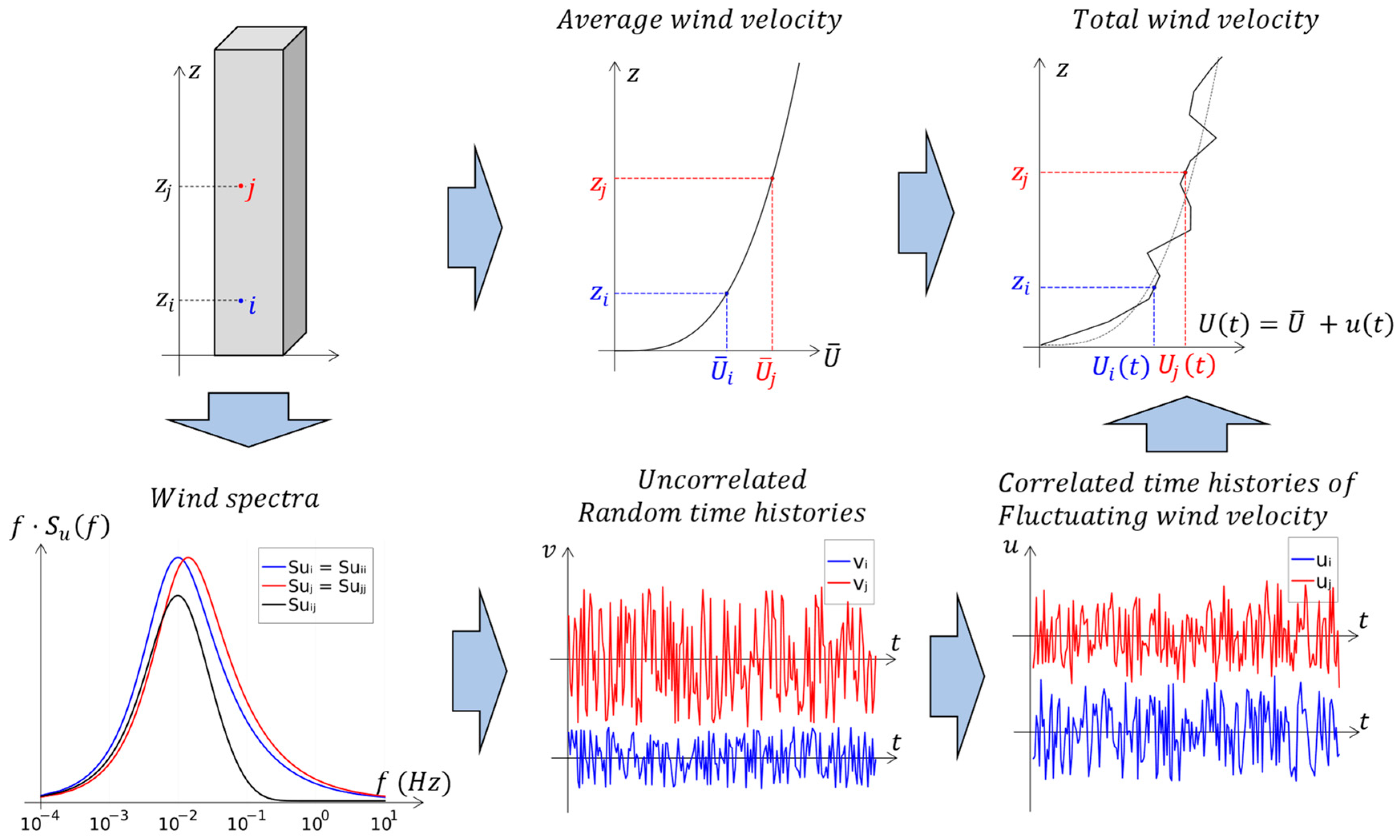
2.1. Dynamic Analysis of a Building Under Wind Action

For a system with multiple DoFs, the equation of motion is given by the following:

$$\mathbf{M}\ddot{\mathbf{y}}+\mathbf{C}\dot{\mathbf{y}}+\mathbf{K}\mathbf{y}={\mathbf{f}}_{\mathbf{e}},$$

(1)

where $\mathbf{M}$, C, and $\mathbf{K}$ are, respectively, the mass, damping, and stiffness matrices of the structure; $\ddot{\mathbf{y}}$, $\dot{\mathbf{y}}$, and $\mathbf{y}$ are, respectively, the vectors of accelerations, velocities, and displacements; and ${\mathbf{f}}_{\mathbf{e}}$ is the vector of external acting forces.

For a system with linear behavior in which few vibration modes are excited (e.g., elevated structures under wind action), the problem can be simplified into these few modes and analyzed using the mode superposition method, in which for each mode, the equation of motion is given by the following:

$$m_i\ddot{y}+c_i\dot{y}+k_{i}y={f_e}_i,$$

(2)

where $\ddot{y}$, $\dot{y}$, and $y$ are, respectively, the modal acceleration, velocity, and displacement associated with the ith mode, and $m_i$, $c_i$, $k_i,$ and ${f_e}_i$ are, respectively, the generalized modal mass, damping, stiffness, and force of the ith mode, given by the following:

$$m_i={\mathbf{\varphi }}_{\mathrm{i}}^{\mathrm{T}}\mathbf{M}{\mathbf{\varphi }}_{\mathrm{i}},$$

(3a)

$$c_i={\mathbf{\varphi }}_{\mathrm{i}}^{\mathrm{T}}\mathbf{C}{\mathbf{\varphi }}_{\mathrm{i}},$$

(3b)

$$k_i={\mathbf{\varphi }}_{\mathrm{i}}^{\mathrm{T}}\mathbf{K}{\mathbf{\varphi }}_{\mathrm{i}},$$

(3c)

$${f_e}_i={\mathbf{\varphi }}_{\mathrm{i}}^{\mathrm{T}}{\mathbf{f}}_{\mathbf{e}},$$

(3d)

where ${\mathbf{\varphi }}_{\mathrm{i}}$ represents the eigenvector of the ith mode.

Dividing Equation (2) by the generalized mass and rewriting the damping in terms of the structural damping ratio ${\zeta }_i=c_i / 2 m_i {\omega }_i$, the equation of motion can be rewritten as follows:

$$\ddot{y}+2{\zeta }_i{\omega }_i\dot{y}+{\omega }_i^{2}y={\displaystyle \frac{{f_e}_i}{m_i}},$$

(4)

where ${\omega }_i$ is the cyclic vibration frequency of the structure for the ith vibration mode.

In this work, only the response in the main wind direction is analyzed as the along-wind loading is essential and has great importance in ensuring the wind-resistant design safety of structures [48,49,50]. However, due to the aerodynamic effects of the wind, high-rise buildings vibrate not only in the along-wind direction but also in the cross-wind and torsional directions [51,52]; these effects will be studied in future works.

Especially in raised structures and given that wind velocity increases with height, to apply forces from wind, a structure is generally divided along the direction of its height [53,54]. In time-domain dynamic analysis, for each section of the building, the drag force acting at time $t$ is given by the following:

$$f_d\left(t\right)={\displaystyle \frac{1}{2}}{\rho }_{air} C_d{A}_{ef}{\left(\overline{U}+u-\dot{y}\right)}^2,$$

(5)

where ${\rho }_{air}$ is the air density; $C_d$ is the drag coefficient;$A_{ef}$ is the effective area of obstruction to the wind passage; and $\overline{U}$ and $u$ are, respectively, the average and fluctuating wind velocity at time $t$. These parameters will be further described below. The parameter $\dot{y}$ is the velocity of the structure in the direction of the force. The addition of the velocity of the structure in the formulation takes the fluid–structure interaction (wind-building) into consideration, resulting in aerodynamic damping.

The drag coefficient depends on the geometry of the building and is generally provided by regulatory standards (Brazilian Standard NBR 6123 [55], Eurocode EN 1991-1-4 [56], and American Standard ASCE 7 [57]) such as the abacus in Figure 1 [55] in which it is verified that for parallelepiped buildings, the coefficient is sensitive to variations in $L_1/L_2$ and $h/L_1$.

Figure 1. Drag coefficient for parallelepiped buildings in low turbulence wind based on [55].

For winds originating from extratropical cyclones, the total wind velocity $U(z,t)$ can be divided into two components, an average velocity $\overline{U}\left(z\right)$ and a fluctuating velocity $u\left(z,t\right)$. Figure 2 illustrates the procedure used to calculate the velocities.

Figure 2. Procedure adopted to obtain wind velocities.

The average component is considered constant over time and variable over height according to the characteristics of the building and its surroundings, given by the following [55]:

$$\overline{U}\left(z\right)=b F_r{\left({\displaystyle \frac{z}{10}}\right)}^p{V}_o,$$

(6)

where $V_o$ is the basic wind velocity, which represents the velocity of a gust lasting 3 s, exceeded on average once in 50 years, measured at a 10 m height above the ground, in an open and flat field [55,56]; $z$ is the height above ground level; $F_r$ is the gust factor, whose value of 0.69 represents a change in gust duration from 3 s to 600 s, the usual time range to obtain the maximum response for dynamic analysis in structures subject to wind action; and $b$ and $p$ are coefficients correlated to the roughness of the surface of the land where the building is located. Equation (6) can also be adjusted for non-flat terrain such as hills or valleys (through a topographic correction factor) and for different return times, if necessary. Parameters $b$ and $p$ adjust the variation in the average velocity along the height presented in Table 1, which also presents the surface drag coefficient $cas$, another parameter of ground roughness that will be used in generating fluctuating velocity time histories.

Table 1. Parameters b, p, and cas for ground roughness categories [55].

Parameter	Ground Roughness Category
	I	II	III	IV	V
p	0.095	0.015	0.185	0.23	0.31
b	1.23	1.00	0.86	0.71	0.50
$cas$ × 103	2.8	6.5	10.5	22.6	52.7

Regarding fluctuating velocity, time histories must be generated for each section of the structural model. The time histories need to individually present characteristics of the natural wind about the statistical parameters and spatial correlation between them [58]. The generation of time histories can be carried out using the auto-regression method, which filters a signal with Gaussian distribution and transforms it into a signal with the required characteristics [59]. Each instantaneous value of $u(z,t)$ is expressed by a finite linear summation of previous values of $u\left(z,t\right)$, plus a random signal with zero mean and specified variance.

To generate these time histories, it is necessary to define the parameters of the wind spectra $S_u$, which describes their frequency content [60]. The most used in the literature and regulatory standards are the Davenport, Harris, and Kaimal spectra. In all of them, there is a greater amount of energy at frequencies below 1.0 Hz (Figure 2), so structures with lower frequencies are more sensitive to this action. The Harris spectrum, used in this work, is given by the following:

$$S_u\left(f\right)={\displaystyle \frac{0.6X_1{\sigma }_u^2}{f{\left(2+X_1^2\right)}^{\frac{5}{6}} }},$$

(7)

where $f$ is the frequency; $X_1$ is the dimensionless frequency,

$$X_1\left(f\right)={\displaystyle \frac{1800f}{ \overline{U}\left(z\right)}};$$

(8)

and ${\sigma }_u^2$ is the variance of the fluctuating velocity:

$${\sigma }_u^2={\displaystyle \frac{20}{3}}Cas {\overline{U}}^2\left(10\right),$$

(9)

The fluctuating velocities at two different points, $i$ and $j,$ are also distinct (Figure 2); however, there is an interdependence between the values called cross or spatial correlation. Since the fluctuation time histories in the time domain are still unknown, cross-correlation can be obtained using the turbulence cross-spectral density function $S_{ij}$ [61]:

$$S_{ij}\left(f\right)={\psi }_u\left({\mathsf{\Delta }}_z,f\right)\sqrt{S_{u,i}\left(f\right)S_{u,j}\left(f\right)},$$

(10)

where ${\psi }_u\left({\mathsf{\Delta }}_z,f\right)$ is the normalized co-spectrum function, which for raised structures, is given by the following:

$${\psi }_u\left({\mathsf{\Delta }}_z,f\right)=\exp \left[-{\displaystyle \frac{f{c}_z\left|z_i-z_j\right|}{\overline{U}\left(10\right)}}{\left({\displaystyle \frac{z_m}{10}}\right)}^{-0.3}\right],$$

(11)

where $z_i$ and $z_j$ are the heights of points $i$ and $j$, respectively; $z_m$ is the average height of the points; and a$c_z$ is the decay coefficient, obtained experimentally or adopted conservatively to be equal to 10 [61].

For a building divided into $n$ sections along the height, a cross-correlation matrix $\mathbf{R}$ of order n can be assembled, whose terms are given by the following:

$$R_{ij}={\int }_0^{\infty }{S}_{ij}df,$$

(12)

Finally, correlated time histories of fluctuating velocities are generated by the following [59]:

$${\mathbf{u}}_{\mathbf{i}}\left(\mathrm{z},\mathrm{t}\right)=\mathbf{Z}{\mathbf{v}}_{\mathbf{i}}\left(\mathrm{z},\mathrm{t}\right),$$

(13)

where $\mathbf{Z}$ is the normalized eigenvectors of $\mathbf{R}$ and ${\mathbf{v}}_{\mathbf{i}}$ is the uncorrelated random time histories generated with variances equal to the eigenvalues of $\mathbf{R}$.

Given that the wind action is a random variable, generally the maximum response ${\delta }_{max}$ is not obtained directly from the peak value presented in the time history response but rather by a relationship between the average value and the standard deviation [62]:

$${\delta }_{max}=\overline{\delta }+g{\sigma }_{\delta },$$

(14)

where $\overline{\delta }$ and ${\sigma }_{\delta }$ are, respectively, the average value and standard deviation of the displacements and $g$ is a peak factor given by the following [62]:

$$g=\sqrt{2\ln \left(f_m T\right)}+{\displaystyle \frac{0.577}{\sqrt{2\ln \left(f_m T\right)}}},$$

(15)

where $f_m$ is the dominant frequency of the response, generally equal to the fundamental frequency of vibration of the structure, and $T$ is the time range to obtain the maximum value (600 s).

Ellis [18] evaluated the fundamental vibration frequencies of 163 rectangular buildings and proposed an equation for their estimation as a function of the height of the building. The same equation is used in Eurocode EN 1991-1-4 [56].

$$f_b={\displaystyle \frac{46}{h}},$$

(16)

where $h$ and $f_b$ are the height in meters and estimated natural frequency in Hertz of the building, respectively.

2.2. Machine Learning Models

Machine learning consists of the process of programming a computer system to make response predictions based on provided data [63]. Each sampling point is composed of predictor variables and target variables. Especially when the sampling plan is large, either due to the quantity or variation range of the variables, it is recommended that a sampling plan be drawn up in advance so that the entire sampling space is satisfactorily represented by a reduced number of samples.

The dataset is randomly divided into two subsets, one for training and the other for model evaluation, a step usually carried out in terms of performance parameters in terms of predicted values. During training, a validation technique is generally used to optimize the model parameters, such as the k-fold cross-validation technique, in which the training data are divided into k parts (folds) and the model is trained iteratively with the samples present in k − 1 folds, with the remaining fold used for pre-evaluation of the generated model. The process is repeated with a new set of training folds and pre-evaluation folds until all k combinations have been used.

If the model’s performance is considered satisfactory, it can be used to predict responses for new values of predictor variables; otherwise, the model must be revised or discarded. The ML techniques to be used in this work are briefly presented below.

2.2.1. k-Nearest Neighbors

The k-NN algorithm is a supervised learning method generally used for classification; however, it can also be used for regression. In both cases, the response prediction is performed based on the closest sample points within the dataset used for training. The distance between two points can be calculated using the p-norm.

In regression problems, the prediction consists of the average of the values of the k nearest neighbors. However, prior treatment of the sample space is recommended if the variables have values with different orders of magnitude, given that those with higher order overshadow the others. In this case, min–max normalization can improve the accuracy of the algorithm.

On the other hand, the algorithm can also suffer from the curse of dimensionality if the number of variables is large. In this case, the distance may present very close values for several points, resulting in inaccurate predictions. To overcome this problem, a size reduction can be performed by discarding the least important variables or improving the contribution of the closer neighbors, or even weighting the variables according to their importance. The weights work in a similar way to min–max normalization, with the exception that the variables start to vary between zero and the assigned weight value; given that the technique uses the distance between the nearest neighbors to predict the responses, the attribution of weights improves prediction by increasing the most important predictor variables.

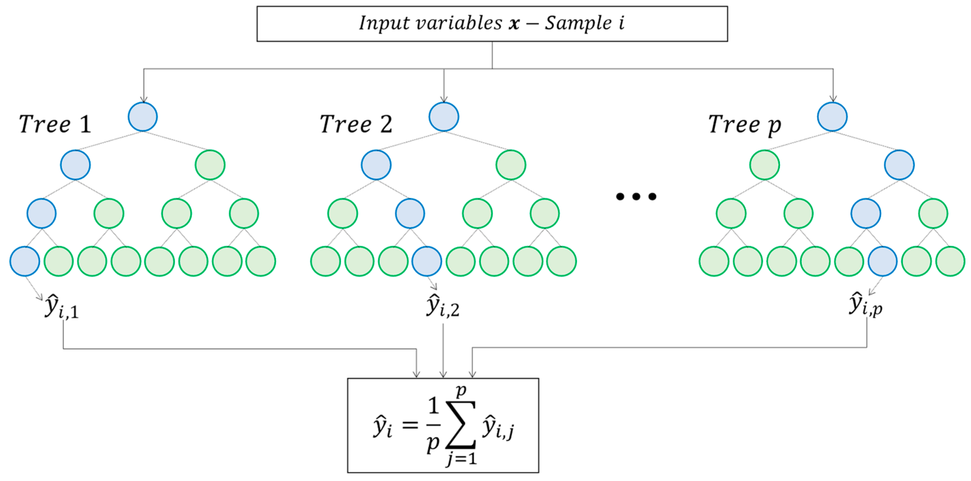
2.2.2. Random Forest

Random forest (RF) is a ML technique that can also be used for classification and regression. The algorithm is called a forest because it consists of a random set of decision trees, whose individual predictions are used to obtain the final, in theory, more accurate, prediction. The technique has already been used in diverse applications such as analyzing the flexural strength of metallic tubes [64], predicting interface friction angles at interfaces involving geomembranes and sand [65], analyzing the ductility requirements for seismic retrofits in concrete reinforced with high-performance fibers [66], and predicting the pressures caused by the fluctuating component of the wind [67].

Classification and regression trees (CARTs) or simple decision trees consist of several connected decision nodes. From the first node (root), the tree is divided into two other nodes based on a decision based on intervals of the predictor variables. Each new node can represent a new decision node or a final node (leaf) in which a value is assigned to the target variable. Individual trees tend to generate an overfitting problem; however, forests tend to minimize this problem. Figure 3 presents a schematic of a random forest for regression.

Figure 3. Random forest regression model for ith sample.

In the random forest model, the hyperparameters are the number of predictor variables considered in node divisions, the minimum number of samples per leaf, the minimum number of samples to divide an internal node, and the number of decision trees.

2.2.3. Support Vector Regression

The support vector machine model (SVM) is based on determining a hyperplane that separates the responses into distinct categories from a set of input variables. The technique can be used in several problems such as structural reliability analysis [68,69,70,71]. When used for regression (Figure 4), it is generally called support vector regression (SVR). SVR searches for the best hyperplane to fit the data within a specified margin of error epsilon ϵ:

$$\left|{\mathrm{y}}_{\mathrm{i}}-{\mathit{w}}_i^T{\mathit{x}}_i\right|\le \mathsf{ϵ},$$

(17)

where ${\mathrm{y}}_i$ is the value of the target variable, ${\mathit{w}}_i$ is the vector of coefficients, and ${\mathit{x}}_i$ is the vector of predictor variables.

Figure 4. Support vector regression model.

However, more complex problems may not present linear behavior, either due to the relationship of the predictor variables with the target variable or due to the spatial dimension, and in these cases, the mapping of variables is carried out through kernel functions, the most used being the Gaussian radial basis kernel function:

$$k\left({\mathit{x}}_i,{\mathit{x}}_j\right)=\exp \left(-\gamma {‖{\mathit{x}}_i-{\mathit{x}}_j‖}^2\right),$$

(18)

Having defined the margin of error, some samples may fit the model while others will remain outside the margin, whose distance is given by $\xi$. Finally, the model results in seeking to minimize the equation

$$MIN{\displaystyle \frac{1}{2}}{\left|\left|\mathit{w}\right|\right|}^2+C \sum _{i=1}^n\left|{\xi }_i\right|,$$

(19)

with the following restrictions:

$$\left|{\mathrm{y}}_{\mathrm{i}}-{\mathit{w}}_i^T{\mathit{x}}_i\right|\le \mathsf{ϵ}+\left|{\xi }_i\right|,$$

(20)

Thus, for the SVR model, the hyperparameters to be optimized are epsilon, kernel gamma, and cost (C) of the variables outside the margin.

2.2.4. Gaussian Process Regression

The Gaussian process for regression (GPR) is a Bayesian method, which implies predictions with uncertainty [72]. Given the set of input random variables $={\left({\mathrm{x}}_{i,j}\right) }_{\begin{array}{c}1 \le i \le m\\ 1 \le j \le n\end{array}}$ and the corresponding observed responses $\mathbf{y}={\left({\mathrm{y}}_i\right) }_{1 \le i \le m}$, where$n$ is the number of predictor variables and $m$ is the number of observations, a Gaussian process $gp(.)$ maps the inputs and outputs through the following relationship [72,73]:

$$\mathbf{y}=gp\left(\mathbf{X}\right)+\mathsf{\epsilon },$$

(21)

where $\mathsf{\epsilon }$ is a Gaussian noise with zero mean and variance ${\sigma }^2$. A Gaussian process is completely defined by its mean function $\mu \left(.\right)$, generally considered constant, and its parameterized covariance function or kernel function $k^{\mathit{\theta }}\left(. , .\right)$. The parameters $\mathbf{\theta }$ of the covariance function, the value of the mean, and the variance of the Gaussian noise can be estimated using the maximum likelihood method:

$$\widehat{\mathbf{\theta }},\widehat{\sigma },\widehat{\mu }=\begin{array}{c}\mathrm{a}\mathrm{r}\mathrm{g}\mathrm{m}\mathrm{a}\mathrm{x}\\ \mathbf{\theta },\sigma ,\mu \end{array}\log \left(\mathrm{p}\left(\mathbf{y}|\mathbf{X}\right)\right),$$

(22)

with

$$\log \left(\mathrm{p}\left(\mathbf{y}|\mathbf{X}\right)\right)\propto -{\mathbf{y}}^{\mathrm{T}}\left({\mathrm{k}}^{\mathbf{\theta }}\left(\mathbf{X},\mathbf{X}\right)+{\sigma }^2{\mathbf{I}}_{\mathrm{m}}\right)\mathbf{y}-\log \left|{\mathrm{k}}^{\mathbf{\theta }}\left(\mathbf{X},\mathbf{X}\right)+{\sigma }^2{\mathbf{I}}_{\mathrm{m}}\right|-\mathrm{m}\mathrm{l}\mathrm{o}\mathrm{g}\left(2\mathsf{\pi }\right),$$

(23)

where $p\left(\mathbf{y}|\mathbf{X}\right)$ is the marginal probability of the observed data and ${\mathbf{I}}_{\mathrm{m}}$ is the identity matrix of order $m$. To estimate the response for a given unobserved input value ${\mathbf{x}}^{\mathbf{*}}$, the prior distribution $gp\left({\mathbf{x}}^{\mathbf{*}}\right)$ is conditioned on the existing observations $gp\left(\mathbf{X}\right)=\mathbf{y}$:

$$gp\left({\mathbf{x}}^{*}\right)|gp\left(\mathbf{X}\right)~\mathcal{N}\left(\widehat{gp}\left({\mathbf{x}}^{*}\right),{\widehat{\sigma }}^2\left({\mathbf{x}}^{\mathbf{*}}\right)\right),$$

(24)

where $\widehat{gp}\left({\mathbf{x}}^{\mathbf{*}}\right)$ and ${\widehat{\sigma }}^2\left({\mathbf{x}}^{\mathbf{*}}\right)$ are, respectively, the mean and variance of the posterior distribution given by the following:

$$\widehat{gp}\left({\mathbf{x}}^{\mathbf{*}}\right)=\widehat{\mu }+k^{\widehat{\mathbf{\theta }}}\left({\mathbf{x}}^{\mathit{*}},\mathbf{X}\right){\left(k^{\widehat{\mathbf{\theta }}}\left(\mathbf{X},\mathbf{X}\right)+{\widehat{\sigma }}^2{\mathit{I}}_m\right)}^{-1}\left(\mathbf{y}-\widehat{\mu }\right),$$

(25)

$${\widehat{\sigma }}^2\left({\mathbf{x}}^{\mathbf{*}}\right)=k^{\widehat{\mathbf{\theta }}}\left({\mathbf{x}}^{\mathbf{*}},{\mathbf{x}}^{\mathbf{*}}\right)-k^{\widehat{\mathbf{\theta }}}\left({\mathbf{x}}^{\mathbf{*}},\mathbf{X}\right){\left(k^{\widehat{\mathbf{\theta }}}\left(\mathbf{X},\mathbf{X}\right)+{\widehat{\sigma }}^2{\mathit{I}}_m\right)}^{-1}{k}^{\widehat{\mathbf{\theta }}}\left(\mathbf{X},{\mathbf{x}}^{\mathbf{*}}\right),$$

(26)

The model’s hyperparameters refer to the parameters of the average function and the kernel function used.

2.2.5. Artificial Neural Network

Artificial neural networks (ANNs) are computational models with the ability to learn, generalize, classify, and organize data through training rules. An artificial neural network consists of multiple layers of neurons in which each neuron in one layer is connected to all neurons in the following layers. The architecture of the neural network consists of an input layer composed of predictor variables, hidden layers, and an output layer with target variables (Figure 5).

Figure 5. Artificial neural network architecture.

Each neuron in a layer following the input layer performs a linear or non-linear transformation on the input values through weights and activation functions layer by layer until the last layer to obtain the responses. Thus, the output value for the kth neuron of a layer ${\mathrm{y}}_{\mathrm{k}}$ will be given by the following:

$${\mathrm{y}}_{\mathrm{k}}=f_a\left(\sum _{i=1}^{n_N}{\mathrm{w}}_{\mathrm{k}\mathrm{i}}{\mathrm{y}}_{\mathrm{i}}+b_i\right),$$

(27)

where $n_N$ is the number of neurons in the previous layer, ${\mathrm{y}}_{\mathrm{i}}$ is the output values of the ith neurons in the previous layer (and input values for the current layer), ${\mathrm{w}}_{\mathrm{k}\mathrm{i}}$ is the weights of the output values of the ith neurons of the previous layer concerning the kth neuron of the current layer, $b_i$ is the bias, and $f_a(.)$ is the adopted activation function.

If the final response obtained presents an unacceptable error, the weights of the neurons are updated in the backpropagation process. Furthermore, in the neural network algorithm, data can be seen by the network more than once (epochs). The hyperparameters to be optimized are the number of hidden layers, the number of neurons in each layer, and learning rate, among others. Different activation functions and optimizers can also be evaluated.

2.2.6. Performance Measurements of Machine Learning Models

To evaluate the results of the ML models, the most used indicators related to target values and those obtained with ML models are the coefficient of determination ($R^2$), mean bias error ($MBE$), mean absolute error ($MAE$), mean squared error ($MSE$), mean percentage error ($MPE$), and mean absolute percentage error ($MAPE$). The closer the coefficient of determination is to unity, the more the responses predicted by the ML models come closer to the expected responses, while for errors, lower values denote a better fit of the model. These indicators are given by the following:

$$R^2=1-{\displaystyle \frac{\sum {\left(y_i-\widehat{y_i}\right)}^2}{\sum {\left(y_i-\overline{y}\right)}^2}}$$

(28a)

$$MBE={\displaystyle \frac{1}{n}}\sum _{i=1}^n\left(\widehat{y_i}-y_i\right)$$

(28b)

$$MAE={\displaystyle \frac{1}{n}}\sum _{i=1}^n\left|Error\right|={\displaystyle \frac{1}{n}}\sum _{i=1}^n\left|y_i-\widehat{y_i}\right|$$

(28c)

$$MSE={\displaystyle \frac{1}{n}}\sum _{i=1}^n{\left(Error\right)}^2={\displaystyle \frac{1}{n}}\sum _{i=1}^n{\left(y_i-\widehat{y_i}\right)}^2$$

(28d)

$$MPE={\displaystyle \frac{1}{n}}\sum _{i=1}^n{P}_{Error}={\displaystyle \frac{1}{n}}\sum _{i=1}^n\left({\displaystyle \frac{y_i-\widehat{y_i}}{y_i}}\right)100$$

(28e)

$$MAPE={\displaystyle \frac{1}{n}}\sum _{i=1}^n\left|P_{Error}\right|={\displaystyle \frac{1}{n}}\sum _{i=1}^n\left|\left({\displaystyle \frac{y_i-\widehat{y_i}}{y_i}}\right)100\right|$$

(28f)

where $y$, $\widehat{y},$ and $\overline{y}$ are, respectively, the target value, the value predicted by the ML model, and the average of the target values, and $n$ is the number of samples from the training or testing subset.

3. Methodology

3.1. Presentation of the Problem

ML techniques are evaluated to predict maximum displacements in buildings under wind loads. For serviceability assessments, the regulatory standards generally indicate that the maximum along-wind displacement and the standard deviation of the characteristic along-wind acceleration of the structure should be used. Moreover, from the known displacement, it is possible to determine all nodal displacements using the mode shape. Once the displacement field is known, it is possible to obtain the deformations, internal forces, and stress in the elements using the constitutive laws that relate to them. Thus, with displacements, it is possible to verify the serviceability limit states directly related to them, as well as use them for ultimate limit states in which internal forces and tensions are required.

Seven predictor variables are used to calculate displacement, five directly associated with the building under analysis and two related to wind (Figure 6):

Figure 6. Illustration of a generic building to be analyzed.

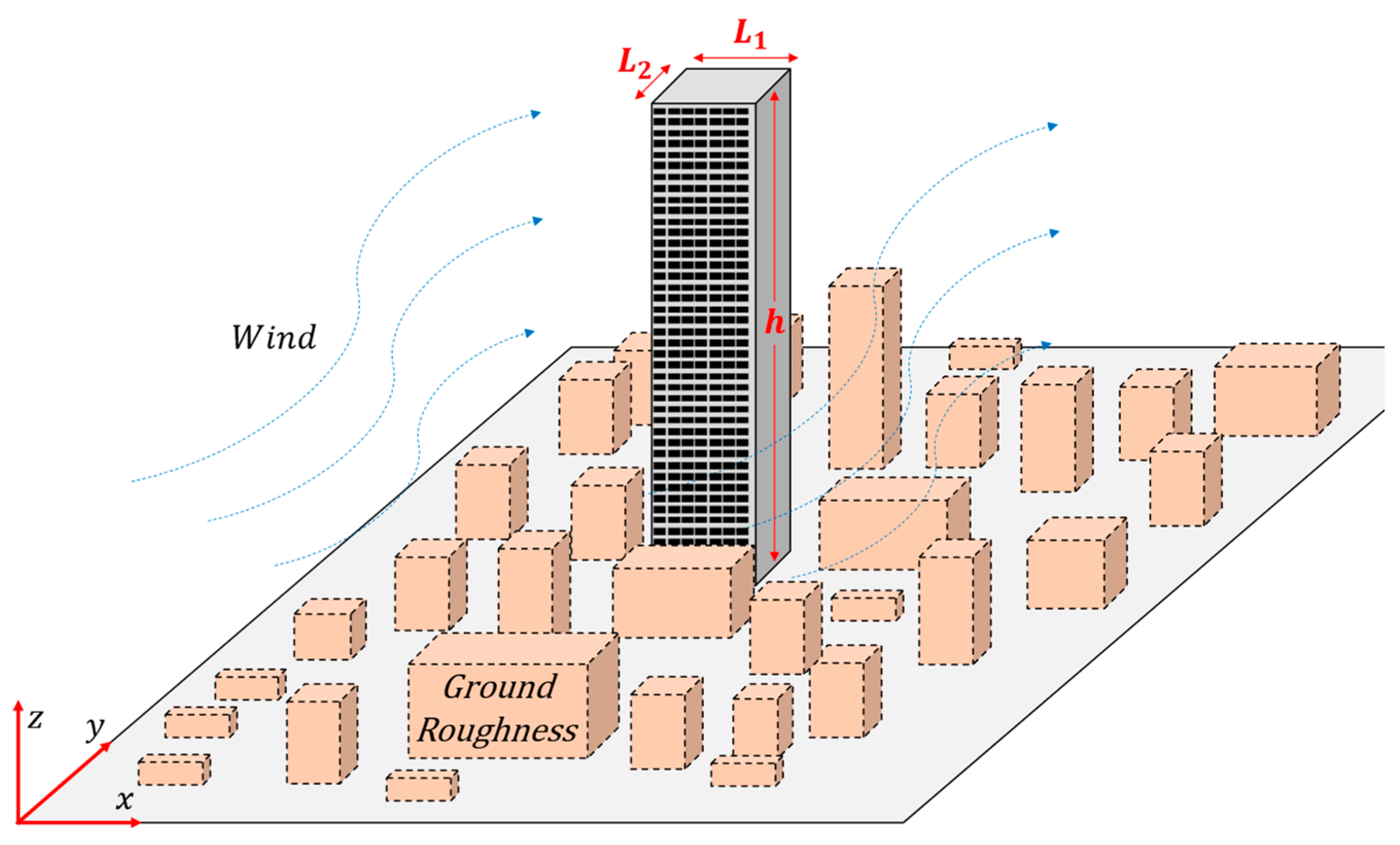
• Height (h)—dimension measured from the ground level to the top of the building. It influences the area obstructing the passage of wind ($A_{ef}$), aerodynamics ($C_d$), and the natural vibration frequency of the building ($f_s=f_1$), and consequently also the dynamic amplification of wind action.
• Width ($L_1$)—horizontal dimension of the building perpendicular to the wind direction. It influences the area obstructing the passage of wind ($A_{ef}$), aerodynamics ($C_d$), and the mass of the structure ($m_s=m_1$).
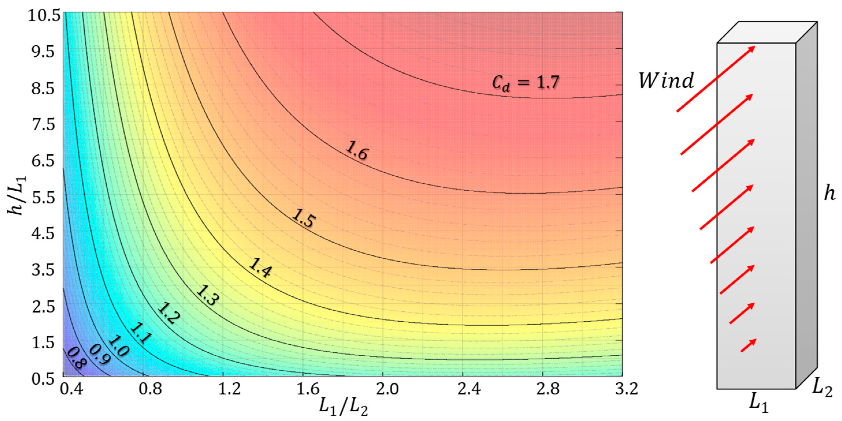
• Length ($L_2$)—horizontal dimension of the building parallel to the wind direction. It influences the aerodynamics ($C_d$) and mass of the structure ($m_s=m_1$).
• Average density of the building ($\rho$)—influences the mass of the structure and, indirectly, the stiffness of the structure ($k_s$) given the correlation between mass and stiffness through frequency ($k_s=4{\pi }^2{m}_s{f}_s^2$).
• Building damping ratio (${\zeta }_s={\zeta }_1$)—influences the dynamic response of the structure, mitigating displacement amplitudes.
• Basic wind velocity ($V_0$)—directly related to the average velocity and indirectly influences the intensity of flow turbulence, according to Equations (6) and (9).
• Ground surface roughness (GR)—represents the obstacles present around the building and is directly correlated to the intensity of flow turbulence. The standards EN 1991-1-4 [56] and NBR 6123 [55] present 5 categories, the first referring to large smooth surfaces and the last referring to the case of terrain covered by numerous, large, high, and closely spaced obstacles. The other categories represent intermediate conditions.

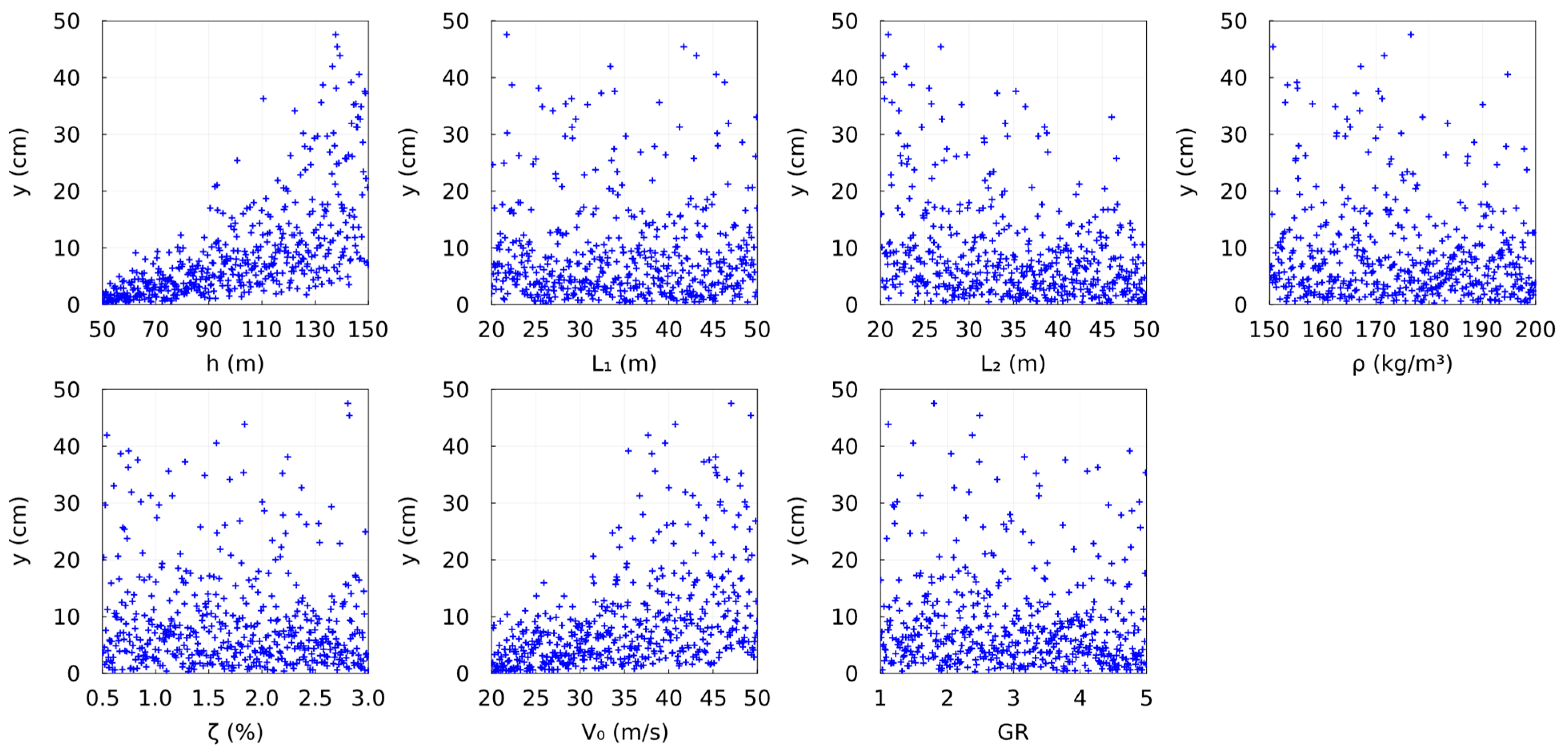
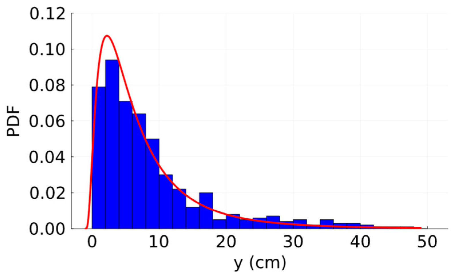
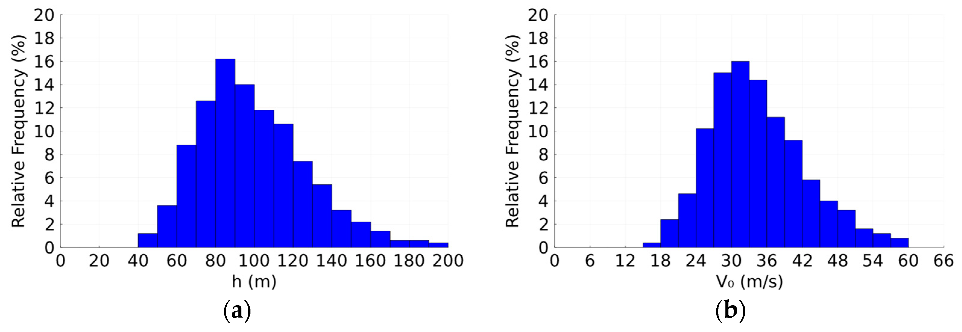
3.2. Sampling and Determination of the Target Variable Values

Figure 7 summarizes the sequence for obtaining the target variable (maximum displacement at the top of the building) from the predictor variables.

Figure 7. Procedure for obtaining the displacement at the top of the building.

To simulate the wind velocity field, the building was divided into sections of approximately 4.0 m along the height according to the corresponding total height, with the average velocity value and the fluctuating velocity time histories being calculated for each section for dynamic analysis. To calculate the average velocity $\overline{U}$, the basic wind velocity $V_o$ and the ground roughness category GR are directly used, with which the parameters given in Table 1 are obtained by interpolation. The fluctuating velocity time histories for each section are generated using the autoregression method [59], and the spatial correlations of the time histories are applied using Equation (13). Also in the fluctuating velocity time histories, the variables $V_o$ and GR used in calculating the parameters of the wind spectra are necessary (Equations (7)–(11)).

In the dynamic analysis, only the contribution of the first mode of vibration was considered, for which the mode shape is taken equal to that of a cantilever beam [74]:

$$\varphi \left(z\right)=\cosh \left(\lambda {\displaystyle \frac{z}{h}}\right)+\cos \left(\lambda {\displaystyle \frac{z}{h}}\right)-\left[{\displaystyle \frac{\sinh \left(\lambda \right)-\sin \left(\lambda \right)}{\cosh \left(\lambda \right)+\cos \left(\lambda \right)}}\right]\left[\sinh \left(\lambda {\displaystyle \frac{z}{h}}\right)-\sin \left(\lambda {\displaystyle \frac{z}{h}}\right)\right]$$

(29)

where $\lambda$ is equal to 1.875 for the first vibration mode.

From the mode shape, the generalized mass of the structure ($m_s$) is estimated by the following [9,75]:

$$m_s=\underset{0}{\overset{h}{\int }}\overline{m}\left(z\right){\varphi }^2\left(z\right)dz$$

(30)

where $\overline{m}\left(z\right)$ is the mass per unit length of the building, given by the following:

$$\overline{m}\left(z\right)=\overline{m}=\rho L_1 L_2$$

(31)

To calculate the drag force in each section of the building at each time interval $f_{d_i}\left(t\right)$, a wind density (${\rho }_{air}$) equal to 1.225 kg/m³ was adopted; the effective area $A_{ef}$ is given by the product between the width (L₁) and the height of the section; and the drag coefficient was obtained from Figure 1 as a function of the dimensions h, L₁, and L₂. And finally, the generalized excitation force is given by the following:

$$f_e\left(t\right)=\sum _{i=1}^{N_s}\varphi \left(z_i\right)f_{d_i}\left(t\right)$$

(32)

where $N_s$ is the number of sections into which the building was divided.

The equation of motion (Equation (4)) is completed by the building’s structural damping ratio (${\mathsf{\zeta }}_s$) and the natural frequency of vibration ${\omega }_s$ (${\omega }_s=2 \pi f_s$), calculated as a function of height using Equation (16). Finally, the maximum displacement at the top of the building is obtained by linear dynamic analysis using Equation (14).

An initial sampling plan for the predictor variables containing 500 sample points was created using the Latin hypercube sampling (LHS) algorithm, which provides uniform and consistent sampling, suitable for the problem analyzed. Once the sampling plan is defined, the maximum displacement at the top of the building is obtained numerically, as previously described. Table 2 presents the mean, the standard deviation, the minimum and maximum values for each predictor variable, and the target variable of the dataset.

Table 2. Statistical parameters of the dataset.

Variables	Abbreviation	Unit	Mean	Std	Min	Max
Building’s height	h	m	99.960	28.836	50	150
Building’s width	L1	m	35.000	8.669	20	50
Building’s length	L2	m	35.018	8.667	20	50
Building’s average density	$\rho$	kg/m3	175.030	14.440	150	200
Building’s damping ratio	$\zeta$	%	1.750	0.722	0.5	3.0
Basic wind velocity	$V_0$	m/s	34.976	8.656	20	50
Ground roughness category	$GR$	----	3.000	1.156	1	5
Maximum displacement	$y$	cm	8.877	8.720	0.274	47.566

The range of values adopted for the dimensions of the buildings aims to include common dimensions in which the dynamic responses present values that cannot be ignored ($f_s<1.0 \mathrm{H}\mathrm{z}$) but are limited to a height of 150 m, a height at which other aeroelastic phenomena could significantly influence the structural behavior. The range of values adopted for the average density of the building includes the values found in some buildings analyzed in previous works [26,27,28], also including a gap adopted arbitrarily. The range of values adopted for the damping ratio includes common values for buildings [15,16,17]; the upper limit was conservatively adopted equal to 3.0%. The basic wind velocity range contains the values commonly presented in regulatory standards for winds originating from extratropical cyclones [55]. The ground roughness category covers all conditions surrounding the building, from the most isolated to the most populated [55,56]. Since LHS was used to generate the samples, the mean of the predictor variables is approximately equal to the mean between the upper and lower limits.

Figure 8 presents the scatterplots of the target variable ($y$) concerning the predictor variables, and Table 3 presents the correlation between the predictor variables and the target variable.

Figure 8. Scatterplots of target variable concerning the predictor variables.

Table 3. Pearson correlation coefficient between target and predictor variables.

	h	L1	L2	ρ	$\mathit{\zeta }$	V0	SR
$y$	0.639	−0.009	−0.295	−0.105	−0.099	0.455	−0.092

The target variable is more strongly correlated with the height of the building (h), with emphasis on the basic wind velocity ($V_0$) and the length of the building (L₂). The positive correlation and greater value for height were expected given that the greater the height, the lower the structure frequency and the greater the dynamic effects of the wind. The positive and significant correlation for basic wind velocity was also expected given that the excitation force is related to the square of the velocity. The negative correlation for the length of the building can be justified by the increase in structural stiffness in the wind direction. On the other hand, the width (L₁), the average density ($\rho$), and the damping ratio ($\zeta$) of the building, and the ground roughness category (GR) show low correlation with the output variable. Although the correlation for these variables is low, they will all be kept for model training, since their influences may be overshadowed by the other variables. For example, it is noted that the dispersion in the responses is large even for the predictor variables h and V₀. Thus, the importance and possibility of exclusion will be assessed directly in the surrogate models.

Figure 9 presents the normalized histogram of maximum displacements at the top of the buildings for the sample set analyzed. A good fit was found with the log-normal probability distribution function, for a significance level of 5% using the chi-square test. Figure 9 also shows the fitted PDF to the data.

Figure 9. Normalized histogram (blue bars) and fitted probability density function (red line) for displacements.

Having identified the best ML models for this problem, for a complementary analysis of the trained models, 500 new sample points were generated, adopting the average values presented in Table 2 for the variables L₁, L₂, $\rho$, $\zeta$, and GR. For variables h and V₀, respectively, samples were generated considering the log-normal and Gumbel-type extreme value probability distribution functions of maximum values, with the means and standard deviations also presented in Table 2. Figure 10 presents the normalized histograms of the new building heights and basic wind velocities generated.

Figure 10. Histogram of relative frequency: (a) height of building h; (b) basic wind velocity V₀.

The responses for the new sampling plan were obtained using the methodology presented previously. Figure 11 presents the scatter plot of the responses as a function of height and velocity.

Figure 11. Scatter plot of displacements as a function of height and velocity.

Finally, the responses are predicted using the best ML models already trained with the first dataset and compared with those obtained from the traditional dynamic analysis.

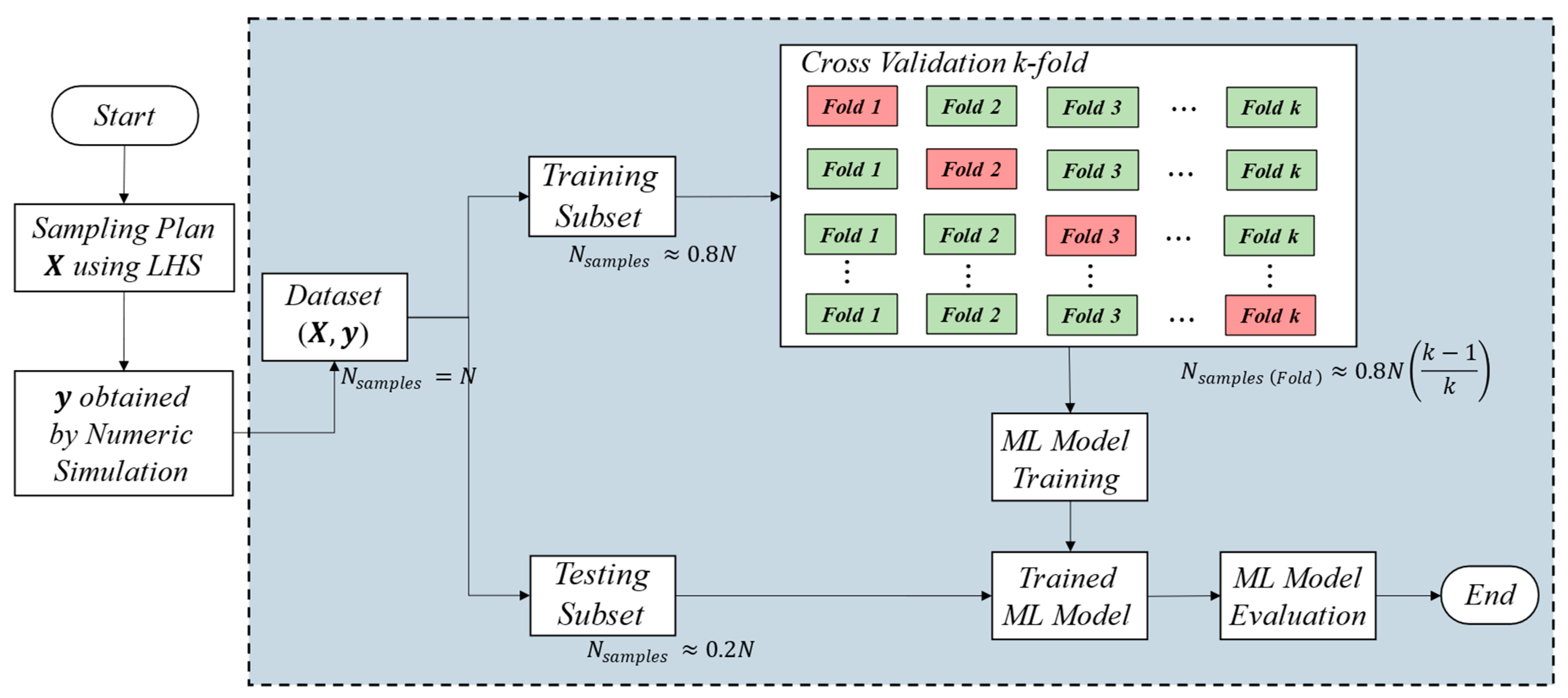
3.3. Machine Learning Models

Five ML techniques for predicting responses are analyzed: k-nearest neighbors (kNNs), random forest (RF), support vector regression (SVR), Gaussian process regression (GPR), and artificial neural network (ANN). The ML models were created according to the flowchart shown in Figure 12; the dataset is divided between training (80%) and testing (20%). Min–max normalization was applied to the predictor variables to avoid problems with their different orders of magnitude.

Figure 12. Flowchart for building a machine learning model.

The training subset is initially used to obtain the best values for the hyperparameters using k-fold cross-validation with 10 folds combined with Bayesian optimization, taking as optimal parameters those that provided the lowest values for the mean squared error MSE (Equation (28c)) they are then used to train the ML model. Bayesian optimization uses Bayesian inference techniques to build a probabilistic model to minimize the MSE. This probabilistic model is used to suggest the next sets of hyperparameters to be evaluated, based on the results of previous evaluations. Finally, with the trained model, the testing subset is used to evaluate the model using the indicators presented in Section 2.2.6.

For the kNN model, the k-neighbors are calculated using the Euclidean distance (p = 2) and were weighted by the inverse of the respective distances; thus, the closer a sample is to the sample to be predicted, the greater its influence on the response, leaving as a hyperparameter, the number, k, of neighbors to be used. However, the importance of the predictor variables is also verified by assigning different weights to them after the normalization stage.

For the GPR model, the zero mean function is generally used; however, 4 functions present in the GaussianProcesses.jl package are tested: Zero (Meanzero), Constant (MeanConst), Linear (MeanLin), and Polynomial (MeanPoly). In addition, 12 kernel functions present in the same package are evaluated: Linear ARD (LinARD), Matern ARD 1/2 (Mat12ARD), Matern Iso 1/2 (Mat12Iso), Matern ARD 3/2 (Mat32ARD), Matern Iso 3/2 (Mat32Iso), Matern ARD 5/2 (Mat52ARD), Matern Iso 5/2 (Mat52Iso), Polynomial (Poly), Rational Quadratic ARD (RQARD), Rational Quadratic Iso (RQIso), Squared exponential ARD (SEARD), and Squared exponential Iso (SEIso).

For the ANN model, 12 activation functions present in Flux.jl are tested: ReLU, CELU, ELU, GELU, Leaky ReLU, LiSHT, Logcosh, Mish, RReLU, SELU, Softplus, and Swish. Seven optimizers from the same package are tested: Descent, Momentum, Nesterov, RMSprop, AdaMax, AMSGrad, and Adabelief.

4. Results and Discussion

Table 4 presents the range of hyperparameters considered for the kNN model and the optimal values verified. A value of 3 was identified for k. In addition, better results were found when different weights were assigned to the predictor variables, indicating that some have a greater influence on the response concerning other variables. The building’s height represents the most important variable, while the width of the building represents the least important. It is noted that all predictor variables contribute to predicting the response.

Table 4. Hyperparameters of the kNN model.

Hyperparameter	Min	Max	Optimal
k	1	5	3
hweight	0.000	5.000	5.0000
L1weight	0.000	5.000	0.3510
L2weight	0.000	5.000	1.9961
$\rho$weight	0.000	5.000	0.7894
$\zeta$weight	0.000	5.000	1.0058
V0weight	0.000	5.000	3.7689
GRweight	0.000	5.000	0.4514

Table 5 presents the range of hyperparameters considered for the RF model and the optimal values identified. For the RF model, the number of predictor variables ($N_{pv}$) to be considered in the node divisions is equal to the totality of predictor variables, the minimum number of samples per leaf (${min}_{SF}$) is equal to 2, the minimum number of samples to split an internal node (${min}_{SS}$) is equal to 3, and the number of trees ($N_{trees}$) is equal to 500. Again, when using all predictor variables, better results are achieved.

Table 5. Hyperparameters of the RF model.

Hyperparameter	Min	Max	Optimal
$N_{pv}$	1	7	7
${min}_{SF}$	2	10	2
${min}_{SS}$	2	10	3
$N_{trees}$	10	1000	500

Table 6 presents the range of hyperparameters considered for the SVR model and the optimal values identified. For the SVR model, values of 0.001, 0.183, and 2000 were obtained for the hyperparameters epsilon (ϵ), gamma (γ), and cost (c), respectively.

Table 6. Hyperparameters of the SVR model.

Hyperparameter	Min	Max	Optimal
ϵ	0.0001	1	0.001
γ	0.0001	3	0.183
c	1	10,000	2000

Table 7 presents the range of hyperparameters considered for the ANN model and the optimal values identified. For the ANN model, the number of hidden layers is equal to 2, with 50 neurons each, and the learning rate is equal to 0.001, and 5000 epochs. As for activation functions and optimizers, there was a better fit with the Leaky ReLU activation function and the Momentum optimizer, as shown in Table 8. However, it is remarkable that the other functions also provide similar results.

Table 7. Hyperparameters of the ANN model.

Hyperparameter	Min	Max	Optimal
Hidden layers	1	6	2
Neurons in hidden layers	5	200	50
Learning rate	0.00001	0.1	0.001
Epochs	10	20,000	5000

Table 8. Average of mean squared errors (cm²).

Activation Function	Optimizer
	Descent	Momentum	Nesterov	RMSprop	AdaMax	AMSGrad	Adabelief
ReLU	1.414	1.090	1.227	1.174	1.359	1.265	1.190
CELU	2.124	1.181	1.204	5.446	2.021	1.547	1.000
ELU	2.114	0.944	1.304	2.119	2.012	1.667	1.919
GELU	1.809	0.931	0.890	1.877	1.646	1.788	1.426
Leaky ReLU	1.776	0.721	1.175	1.373	1.521	1.390	1.118
LiSHT	1.807	0.932	0.849	1.304	1.186	0.854	1.181
Logcosh	2.158	0.787	0.944	1.214	1.400	1.046	0.804
Mish	1.955	0.844	1.225	1.818	1.767	1.516	0.948
RReLU	1.981	1.252	1.413	1.660	2.156	1.886	1.404
SELU	3.117	1.126	2.014	2.486	2.459	1.841	1.074
Softplus	1.985	0.950	1.818	7.385	2.708	1.777	0.872
Swish	1.883	0.785	1.517	1.861	1.839	1.886	0.873

Figure 13 illustrates the variations in MSE, used as a loss function, versus the number of epochs during the training of the optimal network using k-fold cross-validation and for the training and testing datasets.

Figure 13. MSE vs. the number of epochs for training, testing, and validation datasets.

For the GPR model, initially using the mean function Zero, 12 kernel functions were tested (Table 9). It appears that the best kernel for the problem is Rational Quadratic ARD; however, it is remarkable that the Matern ARD 5/2, Squared exponential ARD, and Matern ARD 3/2 functions also presented good results. Using the kernel functions Rational Quadratic ARD, Matern ARD 5/2, Squared exponential ARD, and Matern ARD 3/2, the mean functions were evaluated, the results of which are presented in Table 10. Given the results obtained for the final model, the Rational Quadratic ARD kernel and the mean function Zero were used.

Table 9. Average of mean squared errors (cm²) for evaluated kernel functions.

Kernel Function	MSE	Kernel Function	MSE
Linear ARD	25.734	Matern Iso 5/2	2.145
Matern ARD 1/2	2.861	Polynomial	24.577
Matern Iso 1/2	4.855	Rational Quadratic ARD	0.673
Matern ARD 3/2	0.972	Rational Quadratic Iso	0.969
Matern Iso 3/2	2.312	Squared exponential ARD	0.717
Matern ARD 5/2	0.701	Squared exponential Iso	1.658

Table 10. Average of mean squared errors (cm²) for average functions evaluated.

Mean Function	Kernel Function
	Rational Quadratic ARD	Matern ARD 5/2	Squared Exponential ARD	Matern ARD 3/2
Zero	0.673	0.701	0.717	0.972
Constant	0.673	0.700	0.703	0.972
Linear	0.681	0.709	0.715	0.968
Polynomial	0.681	0.709	0.715	0.968

Figure 14 presents the predicted values for all models compared to the target values for maximum displacement at the top of buildings. Table 11 presents the values of the R², MBE, MAE, MSE, MPE, and MAPE indicators for all models.

Figure 14. Values predicted by the machine learning models × target values: (a) k-nearest neighbors, (b) random forest, (c) support vector regression, (d) artificial neural network, and (e) Gaussian process regression.

Table 11. Performance measurements.

Machine Learning Model	Training						Testing
	R2	MBE (cm)	MAE (cm)	MSE (cm2)	MPE (%)	MAPE (%)	R2	MBE (cm)	MAE (cm)	MSE (cm²)	MPE (%)	MAPE (%)
kNN	1.000	−0.003	0.052	0.007	−0.147	0.676	0.955	−0.518	1.203	3.271	1.088	15.028
RF	0.981	−0.078	0.790	1.932	−5.762	11.060	0.933	−0.673	1.536	5.690	−3.734	20.901
GPR	0.999	0.000	0.149	0.045	−0.038	2.661	0.995	0.111	0.416	0.379	−0.993	8.145
SVR	0.994	−0.069	0.290	0.542	1.064	4.027	0.990	0.024	0.472	0.633	−0.322	8.767
ANN	0.999	0.001	0.150	0.046	−0.140	2.995	0.990	−0.004	0.463	0.653	−1.947	5.941

For the testing set, considering the coefficient of determination R², the GPR model presents the best result, with a value equal to 0.995, indicating good accuracy in predicting responses, while the SVR, ANN, kNN, and RF models presented values equal to 0.990, 0.990, 0.955, and 0.933, respectively; although lower, they still indicate a good fit.

Considering the MBE indicator, which is associated with a systematic error that can occur in the models due to incorrect assumptions, the ANN model presented a lower value (−0.004cm), followed by the SVR, GPR, kNN, and RF models with 0.024 cm, 0.111 cm, −0.518 cm and −0.673 cm, respectively. Positive values for the MBE indicate that the model has a bias toward making predictions with values higher than the target values, and negative values for the MBE indicate the opposite. Thus, it appears that the ANN and SVR models have a bias very close to zero, indicating that the predictions are sometimes lower and sometimes higher than the target values; the GPR model is weakly biased toward making predictions higher than the target values; and the kNN and RF models are highly biased toward making predictions lower than the target values.

Considering the MAE indicator, which provides a measure accuracy of the models in predicting the target values on a continuous scale, the GPR model presented the best result (0.416 cm), followed by the ANN, SVR, kNN, and RF models with 0.463 cm, 0.472 cm, 1.203 cm, and 1.536 cm, respectively.

Considering the MSE indicator, which also provides a measure accuracy of the models in predicting the target values on a continuous scale but using the average squared difference, the GPR model presented the best result again (0.379 cm²), followed by the SVR, ANN, kNN, and RF models with 0.633 cm², 0.653 cm², 3.271 cm², and 5.690 cm², respectively.

Considering the MPE indicator, which computes the average of percentage errors in predicting target values, the SVR model presented the best result (−0.322%), followed by the GPR, ANN, kNN, and RF models with 0.633%, 0.653%, 3.271%, and 5.690%, respectively. However, unlike MAE and MSE errors, it is noteworthy that in MPE, errors can present positive or negative values, which can distort the accuracy of the model.

Considering the MAPE indicator, in which all differences between the predicted value and the expected value contribute positively, the ANN model presents the lowest value (5.941%), indicating better accuracy, followed by the GPR (8.145%), SVR (8.767%), kNN (15.028%), and RF (20.901%) models.

For all performance indicators considered, the RF model presented the worst performance, followed by the kNN model. The GPR model presented the best performance considering the R², MSE, and MAE indicators, being the second best for the MAPE indicator, in which the ANN model presented the best result; second for the MPE indicator, in which the SVR model presented the best result; and third for the MBE indicator, in which the ANN model presented the best result.

Despite the size of the sample space with few samples, given the number of variables and respective intervals adopted, the ML models were able to make predictions of displacements with satisfactory accuracy, resulting in a good tool for cases where it is necessary to perform multiple analyses such as in structural reliability studies or for predicting responses in any models based on an available dataset.

Having identified that the GPR and ANN models provided the best predictions, both were used to predict the responses of the second dataset generated. Figure 15 presents the predicted values compared to the target values, and Table 12 presents the values of the R², MBE, MAE, MSE, MPE, and MAPE indicators obtained.

Figure 15. Values predicted by the GPR and ANN models for the new dataset.

Table 12. Performance measurements of the new dataset.

Machine Learning Model	R2	MBE (cm)	MAE (cm)	MSE (cm2)	MPE (%)	MAPE (%)
GPR	0.984	0.196	0.414	0.894	−4.744	6.868
ANN	0.991	0.103	0.325	0.455	−2.138	4.561

For both models, the coefficient of determination was higher than 0.98 and the MAE, MSE, MPE, and MAPE errors were low and, in some cases, even lower than those identified in the testing set of previous samples. Both models are weakly biased to make predictions higher than the target values. The good accuracy of the ML models can also be verified through the PDFs generated with the answers obtained through the models. As shown in Figure 16, there is a good fit for both models.

Figure 16. PDFs for target values and values predicted by ML models.

Using PDFs, it is possible to infer the probability of a given response value being exceeded or even define the characteristic value for the response considering a given probability of being exceeded. Figure 17 shows the values for displacements depending on the probability of being exceeded. Considering, for example, a 5.0% probability of being exceeded, we would have values of 20.892 cm, 21.519 cm, and 21.045 cm for the displacements obtained using a dynamic analysis, the ANN model, and the GPR model, respectively, corresponding to errors of 3.00% for the ANN model and 0.73% for the GPR model.

Figure 17. Variation in displacements concerning the probability of being exceeded.

5. Conclusions

Five machine learning techniques were used to predict the maximum displacement at the top of buildings under wind loads, k-nearest neighbors (kNNs), random forest (RF), support vector regression (SVR), Gaussian process regression (GPR), and artificial neural networks (ANNs). It was found that all models can present good results; however, the most accurate are GPR, ANN, and SVR, in that order, whose coefficients of determination were equal to 0.995, 0.990, and 0.990, respectively. Despite being inferior, the kNN and RF models still presented coefficients of determination above 0.9, equal to 0.955 and 0.933, respectively. Considering the errors analyzed, it was found that the GPR, ANN, and SVR models also present the best results.

The kNN and RF models present a simpler formulation compared to the others, which may justify the lower accuracies found. For the kNN model, there was a need to weight the predictor variables, either by the order of magnitude of the variables or by their importance concerning the response variable. The height of the building proved to be the most important variable, followed by the basic wind velocity and the length of the building. For the random forest model, the number of decision trees (500) necessary for better model accuracy stands out.

The SVR model presents an intermediate formulation concerning the other models, consisting only of the optimization of the hyperplane to be used for regression. Despite this, it presented results close to the most complex models (GPR and ANN).

For the ANN model, the need to use two hidden layers of neurons with 50 neurons stands out for better model accuracy and to obtain good results with different activation functions. However, the excellent accuracy obtained in this model, just like that obtained in the GPR model concerning the other models, deserves greater emphasis. Still, in the GPR model, good responses are obtained with different kernel functions.

Using the ANN and GPR models previously trained to predict responses from another sample set, it was verified that the accuracy of both was maintained, and through the PDFs of the responses obtained, it was verified that the models can also be used for analyzing systems in which there are uncertainties in the predictor variables and that multiple analyses are necessary, as in structural reliability and optimization studies.

In this way, it appears that by using machine learning models, it is possible to develop robust models for predicting dynamic responses in buildings under wind loads, representing a viable alternative for faster and less computationally expensive structural analyses.

References

- CTBUH. Tall buildings in 2019: Another record year for supertall completions. CTBUH J. 2020, 1, 42–51. [Google Scholar]
- Iancovici, M.; Ionică, G.; Pavel, F.; Mota, F.; Nica, G.B. Nonlinear dynamic response analysis of buildings for wind loads. A new frontier in the structural wind engineering. J. Build. Eng. 2022, 47, 103708. [Google Scholar] [CrossRef]
- Hegyi, D.; Armuth, M.; Halmos, B.; Marotzy, K. The effect of wind on historical timber towers analyzed by plastic limit analysis in the focus of a collapse. Eng. Fail. Anal. 2022, 134, 105852. [Google Scholar] [CrossRef]
- Hareendran, S.P.; Alipour, A.; Shafei, B.; Sarkar, P. Characterizing wind-structure interaction for performance-based wind design of tall buildings. Eng. Struct. 2023, 289, 115812. [Google Scholar] [CrossRef]
- Avini, R.; Kumar, P.; Hughes, S.J. Wind loading on high-rise buildings and the comfort effects on the occupants. Sustain. Cities Soc. 2019, 45, 378–394. [Google Scholar] [CrossRef]
- Roncallo, L.; Solari, G.; Muscolino, G.; Tubino, F. Maximum dynamic response of linear elastic SDOF systems based on an evolutionary spectral model for thunderstorm outflows. J. Wind Eng. Ind. Aerodyn. 2022, 224, 104978. [Google Scholar] [CrossRef]
- Yaghmaei-Sabegh, S.; Daneshgari, S. Residual displacement ratios of highly damped SDOF systems by considering soft soil conditions. Soil Dyn. Earthq. Eng. 2023, 165, 107741. [Google Scholar] [CrossRef]
- Navarro-Quiles, A.; Laudani, R.; Falsone, G. Effect of uncertain damping coefficient on the response of a SDOF system. Probabilistic Eng. Mech. 2022, 68, 103238. [Google Scholar] [CrossRef]
- Clough, R.W.; Penzien, J. Dynamics of Structures, 3rd ed.; Computers and Structures: Berkeley, CA, USA, 2003. [Google Scholar]
- Jain, A.; Surana, M. Floor displacement-based torsional amplification factors for seismic design of acceleration-sensitive non-structural components in torsionally irregular RC buildings. Eng. Struct. 2022, 254, 113871. [Google Scholar] [CrossRef]
- Vicencio, F.; Alexander, N.A. Seismic Structure-Soil-Structure Interaction between a pair of buildings with consideration of rotational ground motions effects. Soil Dyn. Earthq. Eng. 2022, 163, 107494. [Google Scholar] [CrossRef]
- Surana, M.; Singh, Y.; Lang, D.H. Effect of structural characteristics on damping modification factors for floor response spectra in RC buildings. Eng. Struct. 2021, 242, 112514. [Google Scholar] [CrossRef]
- Wan, J.W.; Li, Q.S.; Han, X.L.; Xu, K. Investigation of structural responses and dynamic characteristics of a supertall building during Typhoon Kompasu. J. Wind Eng. Ind. Aerodyn. 2022, 230, 105209. [Google Scholar] [CrossRef]
- Huang, J.; Chen, X. Uncertainty analysis of inelastic response of high-rise buildings to wind using a reduced-order building model. Eng. Struct. 2023, 288, 116224. [Google Scholar] [CrossRef]
- Cruz, C.; Miranda, E. Evaluation of the Rayleigh damping model for buildings. Eng. Struct. 2017, 138, 324–336. [Google Scholar] [CrossRef]
- Dai, K.; Lu, D.; Zhang, S.; Shi, Y.; Meng, J.; Huang, Z. Study on the damping ratios of reinforced concrete structures from seismic response records. Eng. Struct. 2020, 223, 111143. [Google Scholar] [CrossRef]
- Lago, A.; Trabucco, D.; Wood, A. Damping Technologies for Tall Buildings: Theory, Design Guidance, and Case Studies, 1st ed.; Butterworth-Heinemann: Oxford, UK, 2019. [Google Scholar]
- Ellis, B.R. An assessment of the accuracy of predicting the fundamental natural frequencies of buildings and the implications concerning the dynamic analysis of structures. Proc. Inst. Civ. Eng. 1980, 69, 763–776. [Google Scholar]
- Reynolds, T.; Feldmann, A.; Ramage, M.; Chang, W.; Harris, R.; Dietsch, P. Design parameters for lateral vibration of multi-storey timber buildings. In Proceedings of the International Network on Timber Engineering Research Proceedings, Graz, Austria, 16–19 August 2016. [Google Scholar]
- Tamura, Y.; Suda, K.; Sasaki, A. Damping in buildings for wind resistant design. In Proceedings of the First International Symposium on Wind and Structures, Cheju, Republic of Korea, 26–28 January 2000. [Google Scholar]
- Doddipatla, L.S.; Kopp, G.A. Wind loads on roof-mounted equipment on low-rise buildings with low-slope roofs. J. Wind Eng. Ind. Aerodyn. 2011, 211, 104552. [Google Scholar] [CrossRef]
- Estephan, J.; Chowdhury, A.G.; Irwin, P. A new experimental-numerical approach to estimate peak wind loads on roof-mounted photovoltaic systems by incorporating inflow turbulence and dynamic effects. Eng. Struct. 2022, 252, 113739. [Google Scholar] [CrossRef]
- Alawode, K.J.; Vutukuru, K.S.; Elawady, A.; Chowdhury, A.G. Review of wind loading on roof to wall connections in low-rise light wood-frame residential buildings. J. Wind Eng. Ind. Aerodyn. 2023, 236, 105360. [Google Scholar] [CrossRef]
- Vital, W.; Silva, R.; Morais, M.V.; Sobrinho, B.E.; Pereira, R.; Evangelista Jr, F. Application of bridge information modelling using laser scanning for static and dynamic analysis with concrete damage plasticity. Alex. Eng. J. 2023, 79, 608–628. [Google Scholar] [CrossRef]
- Cluni, F.; Gioffrè, M.; Gusella, V. Dynamic response of tall buildings to wind loads by reduced order equivalent shear-beam models. J. Wind Eng. Ind. Aerodyn. 2013, 123, 339–348. [Google Scholar] [CrossRef]
- Nagase, T. Earthquake records were observed in tall buildings with tuned pendulum mass damper. In Proceedings of the 12th World Conference on Earthquake Engineering, Auckland, New Zealand, 30 January–4 February 2000. [Google Scholar]
- Martinez-Vazquez, P. Wind-induced vibrations of structures using design spectra. Int. J. Adv. Struct. Eng. 2016, 8, 379–389. [Google Scholar] [CrossRef]
- Braun, A.L.; Awruch, A.M. Aerodynamic and aeroelastic analyses on the CAARC standard tall building model using numerical simulation. Comput. Struct. 2009, 87, 564–581. [Google Scholar] [CrossRef]
- Pietrosanti, D.; De Angelis, M.; Basili, M. A generalized 2-DOF model for optimal design of MDOF structures controlled by Tuned Mass Damper Inerter (TMDI). Int. J. Mech. Sci. 2020, 185, 105849. [Google Scholar] [CrossRef]
- Ma, J.; Zou, W.; Bai, G. Analysis of random wind-induced response of isolation structure with viscoelastic damper and TMD. J. Wind Eng. Ind. Aerodyn. 2022, 230, 105178. [Google Scholar] [CrossRef]
- Lei, Z.; Liu, G.; Yang, Q.; Law, S.S.; Li, Y.; Cui, T. Experimental investigation on vibration suppression of a new prestressed TMD for wind turbine towers. Thin-Walled Struct. 2024, 202, 112080. [Google Scholar] [CrossRef]
- Xiang, Y.; Tan, P.; He, H.; Yao, H.; Zheng, X. Pendulum tuned mass damper (PTMD) with geometric nonlinear dampers for seismic response control. J. Sound Vib. 2024, 570, 118023. [Google Scholar] [CrossRef]
- Farsijani, D.; Gholam, S.; Karampour, H.; Talebian, N. The impact of the frequency content of far-field earthquakes on the optimum parameters and performance of tuned mass damper inerter. Structures 2024, 60, 105925. [Google Scholar] [CrossRef]
- Marrazzo, P.R.; Montuori, R.; Nastri, E.; Benzoni, G. Advanced seismic retrofitting with high-mass-ratio Tuned Mass Dampers. Soil Dyn. Earthq. Eng. 2024, 179, 108544. [Google Scholar] [CrossRef]
- Li, C.; Pan, H.; Cao, L. Pendulum-type tuned tandem mass dampers-inerters for crosswind response control of super-tall buildings. J. Wind Eng. Ind. Aerodyn. 2024, 247, 105706. [Google Scholar] [CrossRef]
- Fan, M.Y.; Li, W.J.; Luo, X.L.; Shui, Q.X.; Jing, L.Z.; Gu, Z.L.; Yu, C.W. Parameterised drag model for the underlying surface roughness of buildings in urban wind environment simulation. Build. Environ. 2022, 209, 108651. [Google Scholar] [CrossRef]
- LI, B.; Jiang, C.; Wang, L.; Liu, J. Wind tunnel study on influences of morphological parameters on drag coefficient of horizontal non-uniform buildings. Build. Environ. 2022, 207, 108412. [Google Scholar] [CrossRef]
- Evangelista, F., Jr.; Almeida, I.F. Machine learning RBF-based surrogate models for uncertainty quantification of age and time-dependent fracture mechanics. Eng. Fract. Mech. 2021, 258, 108037. [Google Scholar] [CrossRef]
- Evangelista, F., Jr.; García, N.A. A polynomial chaos expansion approach to the analysis of uncertainty in viscoelastic structural elements. DYNA: Revista de la Facultad de Minas. Universidad Nacional de Colombia. Sede Medellín 2016, 83, 172–182. [Google Scholar] [CrossRef]
- Silva, V.P.; Carvalho, R.D.A.; Rêgo, J.H.D.S.; Evangelista Jr, F. Machine Learning-Based Prediction of the Compressive Strength of Brazilian Concretes: A Dual-Dataset Study. Materials 2023, 16, 4977. [Google Scholar] [CrossRef]
- Lima, J.P.S.; Evangelista Jr, F.; Soares, C.G. Hyperparameter-optimized multi-fidelity deep neural network model associated with subset simulation for structural reliability analysis. Reliab. Eng. Syst. Saf. 2023, 239, 109492. [Google Scholar] [CrossRef]
- Wang, X.; Li, Z.; Shafieezadeh, A. Seismic response prediction and variable importance analysis of extended pile-shaft-supported bridges against lateral spreading: Exploring optimized machine learning models. Eng. Struct. 2021, 236, 112142. [Google Scholar] [CrossRef]
- Demertzis, K.; Kostinakis, K.; Morfidis, K.; Iliadis, L. An interpretable machine learning method for the prediction of R/C buildings’ seismic response. J. Build. Eng. 2023, 63, 105493. [Google Scholar] [CrossRef]
- Lin, P.; Hu, G.; Li, C.; Li, L.; Xiao, Y.; Tse, K.T.; Kwok, K.C. Machine learning-based prediction of crosswind vibrations of rectangular cylinders. J. Wind Eng. Ind. Aerodyn. 2021, 211, 104549. [Google Scholar] [CrossRef]
- Bright, I.; Lin, G.; Kutz, J.N. Compressive sensing based machine-learning strategy for characterizing the flow around a cylinder with limited pressure measurements. Phys. Fluids 2013, 25, 127102. [Google Scholar] [CrossRef]
- Weng, Y.; Paal, S.G. Machine learning-based wind pressure prediction of low-rise non-isolated buildings. Eng. Struct. 2022, 258, 114148. [Google Scholar] [CrossRef]
- Lin, P.; Ding, F.; Hu, G.; Li, C.; Xiao, Y.; Tse, K.T.; Kwok, K.C.S.; Kareem, A. Machine learning-enabled estimation of crosswind load effect on tall buildings. J. Wind Eng. Ind. Aerodyn. 2022, 220, 104860. [Google Scholar] [CrossRef]
- Wang, Y.; Li, M.; Yang, Y. Prediction of along-wind loading on tall building based on two-dimensional aerodynamic admittance. J. Wind Eng. Ind. Aerodyn. 2023, 238, 105439. [Google Scholar] [CrossRef]
- Li, S.; Li, X.; Yang, Q.; Zou, Y.; Hui, Y.; Wang, Y.; Su, Y.; Zeng, J.; Liao, Z. Modeling the along-wind loading on a high-rise building considering the turbulence scale effects in the wind tunnel tests. J. Build. Eng. 2024, 88, 109063. [Google Scholar] [CrossRef]
- Xu, L.; Spence, S.M.J. Collapse reliability of wind-excited reinforced concrete structures by stratified sampling and nonlinear dynamic analysis. Reliab. Eng. Syst. Saf. 2024, 250, 110244. [Google Scholar] [CrossRef]
- Choi, S.W.; Seo, J.H.; Lee, H.M.; Kim, Y.; Park, H.S. Wind-induced response control model for high-rise buildings based on resizing method. J. Civ. Eng. Manag. 2015, 21, 239–247. [Google Scholar] [CrossRef]
- Zeng, J.; Zhang, Z.; Li, M.; Li, S. Across-wind fluctuating aerodynamic force acting on large aspect-ratio rectangular prisms 2023. J. Fluids Struct. 2023, 121, 103935. [Google Scholar] [CrossRef]
- Li, Z.; Huang, G.; Chen, X.; Zhou, Y.; Yang, Q. Wind-resistant design and equivalent static wind load of base-isolated tall building: A case study. Eng. Struct. 2020, 212, 110533. [Google Scholar] [CrossRef]
- Gu, D.; Kareem, A.; Lu, X.; Cheng, Q. A computational framework for the simulation of wind effects on buildings in a cityscape. J. Wind Eng. Ind. Aerodyn. 2023, 234, 105347. [Google Scholar] [CrossRef]
- Associação Brasileira de Normas Técnicas (ABNT). Forças Devidas ao Vento em Edificações; NBR 6123—Wind Loads on Buildings; Brazilian Association for Technical Codes: Rio de Janeiro, Brazil, 2023. (In Portuguese) [Google Scholar]
- EN 1991-1-4:2005; Eurocode1: Actions on Structures—Part 1–4: General Actions—Wind Actions. CEN: Brussels, Belgium, 2005.
- ASCE. Minimum Design Loads for Buildings and Other Structures; ASCE Standard; ASCE: New York, NY, USA, 2016; pp. 7–16. [Google Scholar]
- Yan, B.; Shen, R.; Li, K.; Wang, Z.; Yang, Q.; Zhou, X.; Zhang, L. Spatio-temporal correlation for simultaneous ultra-short-term wind speed prediction at multiple locations. Energy 2023, 284, 128418. [Google Scholar] [CrossRef]
- Buchholdt, H.A. An Introduction to Cable Roof Structures, 2nd ed.; Thomas Telford: London, UK, 1999. [Google Scholar]
- Blessmann, J. O Vento Na Engenharia Estrutural, 2nd ed.; Editora da UFRGS: Porto Alegre, Brazil, 2013. [Google Scholar]
- Simiu, E.; Scanlan, R.H. Wind Effects on Structures: Fundamentals and Applications to Design, 3rd ed.; John Wiley: New York, NY, USA, 1996. [Google Scholar]
- Davenport, A.G. The application of statistical concepts to the wind loading of structures. Proc. Inst. Civ. Eng. 1961, 19, 449–472. [Google Scholar] [CrossRef]
- Géron, A. Hands-On Machine Learning with Scikit-Learn, Keras, and TensorFlow, 2nd ed.; O’Reilly Media: Sebastopol, CA, USA, 2019. [Google Scholar]
- Seghier, M.E.A.B.; Plevris, V.; Solorzano, G. Random forest-based algorithms for accurate evaluation of ultimate bending capacity of steel tubes. Structures 2022, 44, 261–273. [Google Scholar] [CrossRef]
- Tanga, A.T.; Araújo, G.L.S.; Evangelista, F., Jr. A comparison between geomembrane-sand tests and machine learning predictions. Geosynth. Int. 2024, 1–14. [Google Scholar] [CrossRef]
- Abellán-García, J.; Guzmán-Guzmán, J.S. Random forest-based optimization of UHPFRC under ductility requirements for seismic retrofitting applications. Constr. Build. Mater. 2021, 285, 122869. [Google Scholar] [CrossRef]
- Li, J.; Zhu, D.; Li, C. Comparative analysis of BPNN, SVR, LSTM, Random Forest, and LSTM-SVR for conditional simulation of non-Gaussian measured fluctuating wind pressures. Mech. Syst. Signal Process. 2022, 178, 109285. [Google Scholar] [CrossRef]
- Hariri-Ardebili, M.A.; Pourkamali-Anaraki, F. Support vector machine-based reliability analysis of concrete dams. Soil Dyn. Earthq. Eng. 2018, 104, 276–295. [Google Scholar] [CrossRef]
- Roy, A.; Manna, R.; Chakraborty, S. Support vector regression based metamodeling for structural reliability analysis. Probabilistic Eng. Mech. 2019, 55, 78–89. [Google Scholar] [CrossRef]
- Chocat, R.; Beaucaire, P.; Debeugny, L.; Lefebvre, J.P.; Sainvitu, C.; Breitkopf, P.; Wyart, E. Damage tolerance reliability analysis combining Kriging regression and support vector machine classification. Eng. Fract. Mech. 2019, 216, 106514. [Google Scholar] [CrossRef]
- Wang, Y.; Xie, B.; Shiyuan, E. Adaptive relevance vector machine combined with Markov-chain-based importance sampling for reliability analysis. Reliab. Eng. Syst. Saf. 2022, 220, 108287. [Google Scholar] [CrossRef]
- Lima, J.P.S.; Evangelista Jr, F.; Soares, C.G. Bi-fidelity Kriging model for reliability analysis of the ultimate strength of stiffened panels. Mar. Struct. 2023, 91, 103464. [Google Scholar] [CrossRef]
- Hebbal, A.; Brevalt, L.; Balesdent, M.; Talbi, E.; Melab, N. Multi-fidelity modeling with different input domain definitions using Deep Gaussian Processes. Struct. Multidiscip. Optim. 2021, 63, 2267–2288. [Google Scholar] [CrossRef]
- Blevins, R.D. Formulas for Natural Frequency and Mode Shape, 1st ed.; Van Nostrand Reinhold Company: New York, NY, USA, 1979. [Google Scholar]
- Holmes, J.D. Wind Loading of Structures, 3rd ed.; CRC Press: Boca Raton, FL, USA, 2015. [Google Scholar]
Disclaimer/Publisher’s Note: The statements, opinions and data contained in all publications are solely those of the individual author(s) and contributor(s) and not of MDPI and/or the editor(s). MDPI and/or the editor(s) disclaim responsibility for any injury to people or property resulting from any ideas, methods, instructions or products referred to in the content. |
© 2024 by the authors. Licensee MDPI, Basel, Switzerland. This article is an open access article distributed under the terms and conditions of the Creative Commons Attribution (CC BY) license (https://creativecommons.org/licenses/by/4.0/).