Abstract
Diameters for drainage stacks and vent lines within high-rise building drainage systems are determined by consulting building standard agencies’ design codes. While these are critical design decisions, codes are based upon dated research (1940s to 1970s), which has numerous inherent limitations, and the methodologies employed within the codes are unclear. Thus, a new methodology is presented which is based upon an analogy with other forms of multiphase flow transport systems. This methodology assumes, as a pre-condition, that flows of air and the flow of water within the stack are reasonably steady over time. Component diameters must then be chosen which ensure an acceptably large air supply or air–water flow ratio, and an acceptably small pressure excursion within the stack. Two ways to implement this methodology are presented: an ‘explicit approach’, in which component diameters are directly calculated using empirical correlations, and an ‘implicit approach’, in which component diameters are determined by iteration, using a hydraulic model. The methodology pre-conditions of the approach are then discussed. The physical geometry of the stack and branches tends to promote steady water flow but to render air flow very susceptible to temporary interruptions. A need to maintain the air pathway within high-rise drainage systems using components to supplement the air feed drawn in through the roof vent as required is highlighted.
1. Introduction
1.1. Historical Development
Vertical wastewater systems transport the waste produced within multi-storey buildings (contaminated water, air and solids) to ground level for onwards treatment and disposal. Designs for these systems are typically developed by consulting building standards agencies’ design codes. These codes have their origins in a series of exploratory studies and debates which commenced in the 1920s and continued until the 1970s. An initial report by Whipple [1] described a need to standardize wastewater system design and to size the system components appropriately. A later body of work by Hunter [2] introduced a concept of a nominal peak water flowrate or a ‘design flowrate’ for wastewater systems, based upon a probabilistic analysis of appliance discharges. A set of seminal studies were then carried out in the 1950s–1970s by the UK Building Research Station (BRS; now BRE) and the US National Bureau of Standards (NBS; now NIST), by Wise and Croft 1954 [3], Wise, 1954 [4], Wyly and Eaton, 1961 [5], Lilywhite and Wise, 1969 [6], Verma et al., 1976 [7] and Wyly et al. 1975 [8]. These studies resulted in the creation of the methodologies for wastewater pipe sizing and layout which remain in use within the construction industry to this present day.
There is, however, a growing trend in the construction industry to build high-rise and ‘supertall’ structures [9]. For such structures several significant limitations in seminal studies and contemporary design codes become apparent. Firstly, experimental test systems were of limited height (often not more than eight floors). Secondly, limited forms of instrumentation were available at the time of test for measuring the multiphase flow generated within these test systems. Thirdly, experimental tests were primarily focussed upon water flow and did not address the issue that the supply of air to the stack may have significant impact on system response. Finally, while water flowrates within test systems vary according to discharge appliance type, elevation, and time, design flowrates used in sizing calculations tend to be based upon water supply. Many of the authors cited above recognise these limitations in their study work. Thus, the dated nature of underlying research, its inherent limitations and the increasing height and complexity of modern buildings has caused the engineering design bases currently in use to become increasingly redundant.
In view of these limitations, there has been a recent expansion in research effort with overall aim being to improve understanding of drainage systems and to refine and to improve existing design codes. Recent research using AIRNET simulation software has suggested that transient discharges of water into tall building stacks are more likely to displace water trap seals [9]. Recent analyses have indicate that design water flowrates, which tend to be based on supply of flow to a stack and not actual flow in a stack, are over-conservative and should be revised downwards (Omaghomi et al. [10], Mohammed et al. [11]). The development of instrumentation to measure the downward annular air–water flow which is prevalent in tall stacks, and the development of models which describe the underlying physics of this flow are ongoing (Xue et al. [12], Stewart et al. [13]). The importance of this research has been highlighted by the recent Sars-Cov-2 (COVID-19) pandemic and substantial evidence linking the spread of pathogens to depletions of water trap seals with tall buildings (e.g., [14,15,16,17]).
It is emphasised that design codes are an invaluable resource to building services engineers. But it must be stressed that design codes do not discuss accuracy or reliability of guidelines which they contain. Nor do they discuss conditions over which guidelines can be expected to provide a guarantee of system performance, or scenarios where exceptions to guidelines might apply. In view of these issues new methods for sizing the stack and vent lines components are presented in this article. Limitations within these methods are identified and discussed in detail. It is hoped that these methods will be of use in informing future codes and standards.
1.2. System Design Criteria
A schematic diagram of a wastewater disposal system for a multi-storey building is shown in Figure 1. The system transports the fluids and solids produced by a range of appliances through a network of branches, a stack, and a drain into a sewer network. The system should ideally satisfy a set of performance criteria also illustrated within Figure 1. These criteria are:
- A requirement to expel all waste (solids, water and air).
- A requirement to function imperceptibly (i.e., without noise, or without vibrations, which may damage pipework).
- A requirement to maintain water in the appliance trap seals (to prevent contamination of habitable space with pathogens).
- A requirement to prevent pressure surges (which may be linked to the need to maintain an air pathway, and to avoid blockages).

Figure 1.
Building Wastewater Drainage System: A Design Process, and a Schematic Diagram of Key System Components.
Figure 1.
Building Wastewater Drainage System: A Design Process, and a Schematic Diagram of Key System Components.

These criteria require satisfying for all forms of discharge scenario imaginable, from single flushes of appliances (e.g., WCs or sinks), random flushes of groups of appliances during periods of ‘heavy’ system use, or ‘near-continuous flow’ events arising from the use of showers and washing machines or the emptying of ‘large volume’ vessels such as bathtubs.
As shown in Figure 1, the system is configured from a set of passive components which include branches, junctions, a wet stack, an optional ‘vent line’ or ‘vent lines’, tees and a drain. (Note the terminology for vent lines varies according to different design codes; the vent line is referred to as the ‘secondary vent’ within [18], the ‘relief vent’ within [19] and the ‘vent stack’ within [20,21]). These components require to be sized, oriented and suitably assembled to achieve an acceptable level of performance at minimal cost. Active components such as air admittance valves (AAVs) or pressure suppression devices (e.g., PAPA devices [22]) may be added to enhance this design at a relatively low additional expense. The passive components affect the general nature of response to discharges (response to continuous flows and transient flows), while the active components will specifically target response to transient events. An effective design will also consider the possibility that drains and sewer pipework at ground level may be subject to overload arising from storm surge events [23,24], thereby impeding flow through drains.
Even for the relatively simple three-floor ‘low rise’ system illustrated by Figure 1, the design process requires a service engineer to make a large number of decisions. It is easy to appreciate how these decisions become increasingly difficult to make as the number of floors in the building increases (i.e., its height increases) due to the increasing numbers of components in the system which require to be assembled and the increasingly large number of possible discharge scenarios which can occur.
2. System Design Codes
To simplify design processes, building standards agencies have thus developed and issued wastewater system design codes (e.g. [18,19,20,21]). These codes contain design procedures which may be summarized according in Figure 2. The engineer supplies key building data (building height, number of floors, etc.), key appliance data (types of appliances and usage patterns of appliances) and preferences regarding the vent system configuration. These inputs are used to establish diameters and slopes for the branches, the stack, the vent line, the drain at the base of the stack and specifications for air admittance valves, through various design rules and look-up tables.
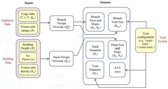
Figure 2.
Design Codes: Design Procedure Overview.
The two primary outputs from this design process are the diameters of the vertical stack and the diameter of the parallel vent line. Focusing on these components, all codes referenced in this article have a set of five general characteristics. These characteristics are:
- Design is performed based upon a nominated maximum water flowrate (i.e., a ‘design flowrate’ ).
- If a design flowrate is input, stack and vent diameters will be output (i.e., stack and vent diameter solutions are guaranteed).
- Stack and vent diameters increase monotonically with ‘stack loading’ (i.e., numbers of appliances which are connected to the stack).
- Stack and vent size diameters increase weakly with ‘stack loading’ (i.e., small increases in pipe sizes require much larger increases in stack loading).
- Design solutions are assumed to be valid for all flowrates below design flowrate (i.e., stack and vent diameters are valid for ).
These shared characteristics of design codes are illustrated as a set C which is shown in Figure 3a. Increases in ‘stack loading’ generally correspond to increases in the number of appliances connected to each branch of the stack and increases in overall building height. While these characteristics are apparent from a casual inspection of Refs. [18,19,20,21], the methodologies used to establish recommended diameters for the stack and vent lines are unclear.
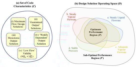
Figure 3.
Design Codes. (a) A set of common characteristics shared by codes, C. (b) An Operating Envelope and a Performance Envelope .
2.1. A Process Analogy
A useful insight into the design methodology may be gained by considering the wastewater system as a form of a multi-phase flow transport system. Examples of such systems include hydrocarbon transport pipelines, nuclear plants, parabolic trough solar devices, and refrigeration devices. In such systems, gas phase feed stream(s) are commingled with a liquid (and/or solid) phase stream(s), sometimes in a controlled manner and sometimes in an uncontrolled manner. This commingling is performed either to transport fluids though an inaccessible environment (to a location where separation and processing is possible), or to promote interaction between fluids (i.e., to encourage heat transfer or chemical reactions).
Multiphase flow transport systems generally have constraints imposed upon their range of operating conditions (‘operating envelopes’). To operate smoothly and efficiently, these systems tend to require that:
- The liquid phase feed stream is reasonably steady;
- The vapor phase feed stream is reasonably steady;
- The vapor phase feed stream is adequately large;
- The system pressure is regulated, i.e., the system operates within a narrow and tolerable pressure band.
The impact of these requirements is schematically illustrated in Figure 3b. The ‘performance envelope’ of a system where performance is acceptable (space ‘P’) becomes much smaller than the space of all operating conditions (the ‘operating envelope space’ ‘O’). Note that the four performance criteria shown in Figure 3b have a considerable overlap; that is to say, the criteria are closely interlinked. Thus, the joint probability of all performance criteria being satisfied may be defined by expressions:
Whereas their joint probability of performance criteria not being satisfied is defined by expressions:
To put Equation (2) into words: if any one of the performance criteria (a), (b), (c) or (d) is not satisfied, it is likely that all four criteria will not be satisfied.
The areas of the four performance regions shown in Figure 3, and the area of the overlap region P shown in Figure 3, are generally sensitive to the size of the pipeline which transports the flowing fluid mixture. It follows from this statement that design engineers will generally try to select the pipeline size for the system which maximizes the size of the overlap region P at the lowest overall cost.
Implications for High-Rise Drainage Systems
It is appropriate to consider high-rise wastewater systems to consider as a form of multiphase flow transport system. These systems admit air and water (and also solids) from appliances in a manner which is uncontrolled, and transport the flow mixture to ground level while attempting to satisfying the performance criteria described above. More formally, these systems must admit flows and remove and dissipate the potential energy which is associated with these flows without converting this potential energy to more disruptive forms of energy.
The discussions above thus imply that the performance of wastewater stacks is linked to the stability of flows of fluids within the system. Moreover, an acceptable flow of the vapour phase in the system (which is in this case air) is also linked to the stability of the pressure within the system. These links can be demonstrated with the aid of Figure 4 and Figure 5. Figure 4 shows a typical ‘flow pattern map’ for vertical, downward air–water flow in circular pipes derived from experimental testing (based loosely on [25]). The normalised velocities which form the axes of this graph are related to phase flowrates by relations = and = . It is apparent that a low air flow encourages the flow of fluids in the pipe as an intermittent ’churn type’ flow, as opposed to an ‘annular flow’. Figure 4 which follows qualitatively illustrates the pressure gradient behaviour for the churn–annular flow transition, [26] (Pressure gradient data for a vertically downward flow are not currently available; however the data shown in Figure 5 illustrate the effect of the transition from intermittent flow to annular flow in an upward flow). This figure suggests that this transition to an intermittent flow from an annular flow causes the system pressure to become highly unstable. Collectively, the two figures suggest that if criterion (c) defined above is not satisfied (i.e., if there is low air flow), criteria (a), (b) and (d) are also unlikely to be satisfied (i.e., there will be likely be unsteady air flow, unsteady water flow and an unsteady system pressure).
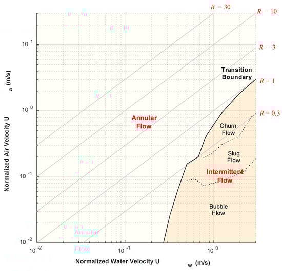
Figure 4.
An example of flow pattern map for vertical downwards air-water pipe flow at atmospheric pressure. The effect of decreasing air flowrate, and decreasing air-water flowrate ratio, is to move the operating conditions within the system from the annular flow region to the intermittent flow region show—adapted from [25].
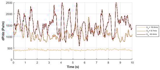
Figure 5.
The impact of a decreasing air flowrate upon pressure gradient fluctuations in an air–water annular flow, as the annular flow–churn-flow transition boundary is traversed (Water velocity = 1 cm s−1. Note that these data are based on a vertical upward annular flow)—adapted from [25].
2.2. A Conditional Methodology
The arguments presented so far allow a conditional methodology for the sizing of the vertical stack and vent line components to be proposed. This methodology assumes, as a precondition, that appropriate action is taken to stabilise the water flow and the air flow within the stack ( and ). This precondition constrains the system within the operating space shown in Figure 3. Provided is satisfied, the selection of stack and vent line diameters which constrain the system within space automatically place the system within the space , and hence place the system within the optimum performance region shown. Thus, the following design methodology statement can be proposed:
where is a nominated demand air flowrate (i.e., a minimum tolerable air flowrate within the stack) and is a nominated tolerable pressure excursion (i.e., maximum tolerable value for the pressure excursion ). Note that the statement requires the specification maximum water flowrate for the system, i.e., a ‘design flowrate’, which shall be denoted as .
It is apparent from Figure 3 that parameter (the minimum air flowrate required to avoid an intermittent flow and to ensure the system operates with an annular flow regime) increases as a function of the water flowrate . This dependency suggests that a simpler design methodology statement can be written by considering the air–water flowrate parameter in place of parameter . Thus, a revised methodology statement is:
where is a nominated minimum tolerable air flowrate ratio (a ‘demand’ ratio), is the minimum achievable air–water flowrate ratio for all possible scenarios of flow in the system (, ) and is a maximum observed pressure excursion for all possible scenarios of flow in the system (, ). The need to select the smallest diameters possible is an economic decision, driven by piping material costs and space constraints.
2.2.1. Implementation
This design methodology lends itself naturally to implementation using steady-state hydraulic modelling techniques. Two such modelling approaches will be presented in Section 3 and Section 4 which follow. The first of these procedures is a relatively simple ’explicit approach’ in which the diameters are directly calculated, whereas the second approach is a more sophisticated ‘implicit approach’ where diameters are indirectly derived with the aid of a hydraulic model. Both these procedures are transparent and they integrate the supply of air to the stack and the most extreme pressure within the stack into calculations in a way which is not evident from a consultation of design codes. The two methods are compared in Section 5; the underlying pre-condition that there must be stable flows of air and water within the system is then revisited in Section 6.
2.2.2. A Note on ‘Fixture Units’ and ‘Fixture Unit Density’
The layouts of floors and locations and the types of appliances connected to a stack tend to vary with floor height in high-rise buildings. While these effects are accounted for in most standard design code procedures, it is convenient for the purposes of this study to assume uniform floor layouts so that the simplifying concept of a ‘fixture unit density’ can be introduced. If appliances (or, equivalently, groups of appliances) of one single type are connected to a stack of height at regular vertical intervals it follows that:
where is the total number of appliances in the building, is its total number of fixture units, is the building ‘appliance density’ (appliances m−1) and is the building ‘fixture unit density’ (fixture units m−1). The fixture unit approach has its origins in probability theory that is outlined in [27]. This approach provides a simple means of relating the flow characteristics of appliances, with calculated ratings such as are shown in Table 1, to an average maximum discharge flowrate.

Table 1.
Example Fixture Unit Ratings according to BS-EN-12056 Code. Data from [18].
While the ‘fixture unit density approach’ is simplistic it enables the two different methodologies for sizing the stack and the vent lines now presented to be described and analysed in the simplest manner possible.
3. An Explicit Design Approach
The first methodology which will be proposed is an ‘explicit approach’ for the calculation of stack and vent line diameters. In this approach a group of ten input parameters are used to calculate two output parameters, as shown in Figure 6. The inputs are grouped into pairs of ‘loading parameters’ (the stack height and a fixture unit density ), ‘operating parameters’ (an air–water flowrate ratio and a stack suction pressure ), and ‘vent line parameters’ (vent line air flowrate fraction and vent line delivery distance ). The model also requires four empirical constants (two ‘appliance usage’ parameters and and two parameters which characterize an annular flow, and ). These inputs are used to evaluate five intermediate variables (, , , , and ), and the stack and vent line diameters ( and ).
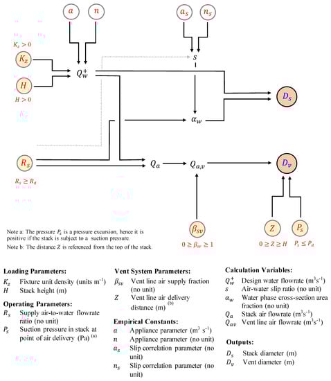
Figure 6.
An Explicit Design Approach. Model input are shown in red and model outputs shown in blue.
The calculation procedure consists of seven steps: the calculation of the five intermediate variables and then the calculation of the output sizes and . Details are as follows:
Step 1. Calculate a maximum water flowrate, (i.e., a design flowrate) using the loading parameters and . and a fixture unit method of the form described in [27]. According to this method, the design flowrate is defined as:
where the parameters and represent characteristics of the discharge appliances and the product represents the total number of fixture units connected to the stack, as defined by Equation (1) above. Typical values for the parameters and are proposed in [28].
Step 2. Calculate a supply air flowrate, based on the design flowrate, and an air–water flowrate ratio, :
The flowrate is the minimum necessary airflow which is required to ensure a stable operation of the system.
Step 3. Calculate a slip ratio for the air–water flowing mixture, . This slip ratio is defined as a ratio of in situ phase flowing velocities = , and is defined by:
where is the air–water flowrate supply ratio, and where and are the slip ratio correlation parameters. Representative values for these parameters, which are valid on condition that there is a steady-state annular flow in the stack, can be obtained from consultation of [5,29].
Step 4. Calculate a maximum acceptable water cross-section fraction for the air–water flow, . This maximum water fraction is derived from the expression:
in which the parameters and are defined as:
and where is the air cross-section fraction, defined as = 1 .
Step 5. Calculate a stack diameter, , using the parameters and obtained in Steps 1 and 4. This diameter is given by:
Equation (11) is based upon a balance of forces within an element of water film adopting an annular flow geometry, as discussed in [28]. In applying this balance, several significant assumptions are made regarding the turbulence of the annular flow within the stack.
Step 6. Calculate the air flowrate which is supplied to the stack through the vent line system, according to:
where is the fraction of the air flow supplied through the vent line. It is assumed that air which is not supplied from the vent line is drawn in through the stack inlet. Thus, it is equivalently possible to define a stack supply fraction, , such that air flowrate supplied to the stack through the stack inlet is given by . Note that = 0 if = 0; this setting for parameter corresponds to a single-stack design where there is no vent line.
Step 7. Calculate a vent line diameter, , based on the vent line supply flowrate . This diameter is estimated using Darcy’s equation:
where is the distance over which ventilating air supplied from the vent line inlet requires to be transported, and is a nominated suction pressure in the stack at the point of delivery ( for < 0 mm H2Og). This parameter can typically be related to the depth of water in a standard trap seal (discussed in e.g., [28,30]).
This explicit approach shares two features with the standard industry design code approaches which are schematically illustrated in Figure 2. Firstly, a design solution is always guaranteed (the nature of the empirical correlations defined above is that any set of input values will always yield meaningful output). Secondly the design is conducted on the basis that there is a maximum flowrate (a design flowrate = ) and it is assumed that the system performs acceptably for all < . In contrast to Figure 2, however, the airflow in the stack and the pressure within the stack have been integrated into the design procedure.
3.1. Procedure Features
The six variable input parameters which are defined in Figure 3 may be compiled to form an input vector = [, , , , , ] and the two outputs may be compiled to form the output vector = [, ]. The nature of the equations employed in the approach means that the entries for the derivative matrix / have properties which are shown in Table 2. Most of the entries in this matrix have a definitive positive or negative polarity. The stack diameter is sensitive to the loading parameters, and and the air-water ratio, . The vent diameter is, on the other hand, sensitive to all six entries in .
Table 2.
Properties of entries within derivative matrix .
The information contained in Table 2 allows several important features of the model to be identified. Firstly, it is observed that the model outputs increase monotonically with the loading parameters and . Since the water flowrate is proportional to and to (Equation (2)), it follows that:
which is to say that the model output increases monotonically with the nominated design flowrate . Note, however, that the design flowrate is merely the largest of a range of water flowrates that the system is required to handle. Evidently, smaller sizes would be preferable according to the procedure, were the system to be operated below its nominated design flowrate ( < ). Thus, these monotonic trends infer that model output contains the largest entries of a set of preferable component sizes.
This observation raises a subtle, but important, point. Methodology statement stipulates that component sizes should be as small as possible (Section 2.2). In order for the entries of to satisfy this requirement, an argument external to the procedure shown in Figure 6 must be applied. An appropriate argument is to assume that undersized pipes which are handling large discharge flowrates will always lead to poorer system performance than oversized pipes which handle low discharge flowrates. While this statement may appear obvious it is not connected to the procedure shown in Figure 6 in any way, nor it is explicitly stated within design codes. Nevertheless this preferential logic requires to be applied in order to be able to consider the model outputs and as minimum pipe sizes.
The entries within the third and fourth columns of Table 2 indicate, additionally, that outputs and will be the smallest sizes possible, if the input parameter is as small as possible and the input parameter is as large as possible. Thus, to satisfy statement , these parameters should be set to the limiting values defined in Section 2.2 above, which are namely:
where is the ‘minimum tolerable flowrate ratio’ and is the ‘maximum tolerable stack pressure excursion’. The modelling approach is thus compatible with the general observations illustrated within Figure 4 and Figure 5. Note that suitable values require to be nominated for parameters and , but are not presented here. In nominating these suitable values, it is assumed that the supply of air to the stack always meets a nominated minimum air demand and that pressure extremes in the stack are always avoided. These are critical assumptions, but are unproven.
Finally, a substitution of Equations (7) and (9) into the Equations (11) and (13) yields the following relationships between the loading parameters and and output component sizes and :
in which , , and are constants and the exponents , , and are functions of the input parameter . Table 3 summarizes the relationships between exponent , , and and , and illustrates representative values for the exponents based on the constant value = 0.5 proposed in [28]. These representative values are all positive but are also all less than unity, indicating that output component sizes have only a weak dependency upon the input loading parameters and . This weakly dependent behaviour is ultimately attributed to the turbulence models which are used to model the flows in the wet and dry part of the stack, as reflected in the use of Equations (7) and (9).
Table 3.
Exponential relations between stack and vent diameters, loading parameters and , and air delivery distance, . Exponent values for nominated input value = 0.5 are also shown.
3.2. Approach Summary
The explicit approach is a straightforward calculation process which shares many of the three characteristic features of design codes which are illustrated in Figure 3a. The model provides guaranteed output solutions which increase monotonically and weakly with a pair of input loading parameters and . However, this approach requires a large number of input parameters to be specified (, , , , , , , ) and makes a relatively large number of assumptions. These assumptions are as follows:
- The fixture unit method as defined by Equation (4) provides a reliable estimate of the design flowrate .
- There is fully developed, steady-state, droplet-free annular downflow within the stack, such that Equation (9) can be applied.
- The supply of air through the stack meets the stipulated necessary minimum demand, and pressure excursions within the stack remain below the maximum tolerable level ( and ).
- Influences that system geometry have upon system performance (e.g., the sizes and orientations of branches, discharge junctions, and the base horizontal drain) can be captured through the remaining model input parameters ().
There is particular concern that these assumptions will cause the model to lose reliability as fixture unit density, stack height, and stack diameter increase. Thus, an alternative design approach in which these critical assumptions can be bypassed is now described.
4. An Implicit Design Approach
An alternative approach to sizing the stack and vent lines components is an implicit approach, which is illustrated within Figure 5. In this implicit approach, a set of four parametric inputs (the two loading parameters and , and candidate stack and vent diameters and ), two input constants ( and ) and two sets of input data that define the geometry of the system and the ‘discharge configuration’ (i.e., the feed of discharge water is delivered to the stack via the appliance branches) are fed into a steady-state hydraulic model. This model is used to calculate two output parameters: a minimum air-to-water flowrate ratio, , and a maximum system pressure excursion, .
To establish stack and vent diameters, the implicit approach must be run iteratively using trail values for the stack diameter and vent diameter, until the outputs and satisfy suitably chosen design criteria. Each iteration cycle consists of four steps, which are as follows:
Step 1. Calculate a design flowrate , using the fixture unit method employed in the explicit approach; that is to say, via equation:
where the constants and reflect appliance loadings and typically adopt values of the order of 0.5 (Step 1 may be bypassed by directly supplying a design flowrate as input to the hydraulic model, as indicated in Figure 7. In this case, the stack height and the design flowrate become independent variables).
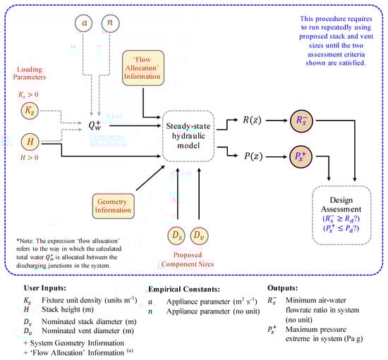
Figure 7.
An Implicit Design Approach. Model inputs are shown in red and model outputs are shown in blue.
Step 2. Calculate the steady-state flowrate ratio profile in the stack, , and a steady-state pressure profile within the stack, , using the calculated design flowrate, the system geometry, and by implementing a steady-state flow hydraulic model. This model is described in further detail below.
Step 3. Extract summary data from the flowrate ratio profiles and pressure profiles, according to the formulae:
Typically, the limit value is obtained at the base of the stack (where the discharge water flowrate has its maximum value), whereas the limit value is obtained downstream of active junctions (where there will be significant suction pressure, due to junction losses).
Step 4. Assess the design by comparing the summary output parameters and against the design criteria. Based on discussions above, it is proposed for acceptable performance that it is necessary that:
i.e., the calculated air-to-water flowrate ratio should exceed a minimum demand ratio, and the maximum pressure deviation should remain below the minimum tolerable demand for pressure excursion.
The implicit approach is fundamentally different to the design code approaches illustrated in Figure 2 and the explicit approach illustrated in Figure 4. Firstly, there is no guarantee that a design solution is to be found, for any given set of inputs. There is also no guarantee that the ‘maximum discharge flow case’ is necessarily a design case: it is possible for a system to fail the assessment process when operated below the design flowrate. Finally, it is not necessarily true that selected component sizes increase monotonically with the loading parameters and . In these respects, the implicit approach is more conservative than the explicit approach; however, the trade-off is that the hydraulic model forming the core of the procedure must be physically accurate. This model is required to predict behaviour of vertical, downwards annular flow within the stack. The key features of this model are now described.
4.1. Steady-State Hydraulic Model
The steady-state hydraulic model which can be implemented within Figure 4 has been presented and discussed in [13]. This model makes use of pressure gradient functions for vertical, downward air–water annular flow to derive a pressure profile within the stack and to establish air flowrates in the branches according to a procedure which is now outlined.
The principle of the model can be most easily described by considering a ‘single-stack’ system (i.e., a stack without a parallel vent line). Such a system has a single inlet pressure boundary and a single outlet pressure boundary (a roof inlet and an outlet to the sewer network). When a steady flow of water is discharged into this stack, air is drawn into it at a steady rate, and is drawn through the stack with a uniform flow profile. This system is required to satisfy the constraint:
where the parameter is the hydraulic pressure gradient (having units Pa m−1). This parameter is a function of the normalised velocities and , the vertical elevation , and, critically, the stack diameter . The parameter is also a function of the stack geometry, and changes particularly rapidly in the vicinity of junctions where water is being discharged into the stack (e.g., [31,32]).
A more complicated balance exists for a vented stack system. A vented stack system as shown in Figure 1 delivers air drawn through the top of the vent line to the stack at multiple locations. Denoting the total number of cross-vents in this design as , there are possible paths along which air can flow between the inlets and the outlet and characteristic air velocities in the system (one air velocity for the stack inlet, and air velocities which are added to these velocities at each cross-vent). There are thus + 1 ways to write equations analogous to Equation (20) applied along a path between an inlet point and the stack base. It is convenient to denote these equations using notation ( = {0, … + 1}), such that:
Within Equation (21) the pressure gradient is a function of air velocities (velocity representing the air drawn in through the top of the stack and air velocities for air drawn in through the cross-vents), the water velocity , the stack diameter , and the vent line diameter . Equation (21) is thus a system of + 1 equations for + 1 unknowns.
4.2. Solution Procedure
As Equation (21) is a system of non-linear equations it must be solved iteratively, using numerical techniques. These techniques require the pressure gradient function to be accurately defined in all regions of the system (particularly within the region of the system where pressure changes rapidly: i.e., at active discharging junctions, at active cross-vents and at the stack base). Moreover, the non-linear nature of the equations means that no solutions, one solution or several feasible solutions for air velocities and pressure profiles may be returned. If several solutions are returned, a ‘best judgement’ must be applied to determine which solution is most appropriate. Typically, the most appropriate solution is the most conservative solution: i.e., the solution resulting in the lowest values for the ratio and highest values for the system pressure .
4.3. Method Summary
The implicit approach is a relatively complicated approach to component sizing that is fundamentally different to the explicit approach described in Section 4 and the design codes approaches as represented within Figure 3a. A design solution is not guaranteed; the method does not ‘design for maximum flow’, and the model output is not necessarily monotonic with appliance loading. However, the implicit approach addresses the following inherent limitations of the explicit approach:
- Air supply is not automatically assumed to meet air demand;
- Stack pressure is not automatically assumed to be adequately regulated;
- Adjustments to system geometry can be directly handled rather than being indirectly handled through the adjustment of model parameters.
The trade-off is increased model complexity, and increased difficulty in model implementation: a potentially large number of flow configurations have to be investigated, with decisions required to be made about how flow is to be allocated within the junctions of the system, to arrive at a design solution.
5. Approach Comparison
Table 4 compares key features of industry standard design codes, the explicit approach proposed in Section 4 and the implicit approach proposed in Section 5. It is evident that parameters which are outputs in the explicit approach (the diameters and ) become input parameters in the implicit approach, and also that constraints imposed upon input parameters in the explicit approach ( = and = ) become assessment criteria in the implicit approach ( ≥ and ≤ ). Both the explicit and the implicit methods assume there are steady-state flows of air and water, but it is not known whether design codes make this same assumption.
Table 4.
A Comparison of Design Approaches.
6. Key Design Premise Revisited
The design approaches described in Section 3 and Section 4 are based upon a precondition of ‘flow stability’ (premise and as defined in Section 2.2). This precondition requires to be satisfied so that systems operate within the ‘optimum performance region’ illustrated in Figure 3. Wastewater stacks generally, however, must process fluids which are discharged in an uncontrolled manner. This inability to control the supply water to the stack places the validity of premise in doubt, and it is appropriate to conclude this article by exploring this issue in closer detail. We propose that the physical geometry of wastewater stacks tends to promote compliance with premise but also tends, temporarily, to cause significant violations of premise .
6.1. Stabilising Effect upon Water Flow
Appliances which are discharged randomly into a wastewater stack tend to have ‘sharply defined’ water flowrate discharge profiles at their outlets as shown, for example, in Figure 7 (data for a typical WC appliance, discussed in [33]). This fact would, upon first consideration, suggest that water flow within the stack is highly variable, such that the stability premise cannot normally be satisfied. However, applies to the stack and not to the branches; and the effect of the appliance branches and the stack itself is to stabilize water flow within the stack, as shown schematically in Figure 8 and Figure 9. These figures demonstrate that:
- Frictional resistances of the branches which connect appliances to the stack have a diffusive effect upon single-flush discharge profiles that increases as branch length increases (Figure 8);
- The commingling of multiple, randomly operated appliance discharges in the stack tends to cause a relative stabilisation of water flowrate (Figure 9);
- The frictional resistance of the stack wall also has a diffusive effect that tends to mitigate sudden changes in water flowrate (Figure 9).

Figure 8.
An example of flow attenuation within a horizontal branch downstream of a flushing WC appliance, as modelled using proprietary DRAINET software (developed by Heriot-Watt University).
Figure 8.
An example of flow attenuation within a horizontal branch downstream of a flushing WC appliance, as modelled using proprietary DRAINET software (developed by Heriot-Watt University).


Figure 9.
The stabilising effect of increasing numbers of discharge appliances upon the normalised water flowrate within a stack , where is the mean water flowrate for appliances. The calculation is based on appliances having a mean duration between discharges of 300 s and a flush profile at the end of the discharge branch, as shown in Figure 8. The effect of flow diffusion in the stack (red line) is schematically illustrated only.

The net result is that discharges which occur randomly and which have sharply defined profiles (Figure 8) transform into a relatively stable water flowrate profile at the stack base (Figure 9). The physical geometry of the system has a significant bearing on this outcome; it is the large length-to-diameter ratio of the branches and the stack itself which steady the water flowrate. When the stack water flowrate is relatively stable it follows from joint probability relationships (Equations (1) and (2)) that the stack air flowrate is also likely to be stable. Thus a system which contains relatively long and thin appliance branches and a relatively long and thin stack has a natural ability to steady the water flow and to steady the air flow.
6.2. Vulnerability to Air Flow Instabilities
The large length-to-diameter ratio of the stack has, however, another important and undesirable consequence. This large ratio makes tall stacks susceptible to ‘upset events’ in which pipe blockages cause brief, but severe, interruptions to air supply. There are a wide range of possible causes of these upset events, and these causes are well documented in the academic literature. Some examples include:
- Wind shear at the top of the stack [22] (which can give rise to suction pressure and encourage air updraft);
- Discharges of solids into the stack [34] (leading to brief interruptions in the air supply);
- Discharges of surfactants within the waste stream (leading to creation of foams at air–water interfaces);
- The falling water curtain at the base of the stack [35] (blocking the air pathway to the horizontal drain);
- Storm surge events [3] (which can affect liquid level in the drains downstream of the stacks and lead to substantial pressure releases).
These events are more likely to occur in tall and heavily-loaded stacks hosting many discharging junctions, and in environments subject to extreme rainfall patterns. Should these events cause temporary but significant instabilities in the air flows, it follows from the joint probability relationships (Equations (1) and (2)) that there will be temporary but significant instabilities in water flows.
6.3. Design Implications
Thus, the physical geometry of a wastewater system—the low diameter-to-length ratio, , of the stack and connecting branches—tends predominantly to promote steady flows of air and water in the stack, but also, for brief instances, to cause flowrates of air and water to become very unstable. This behaviour suggests that systems designed according to the explicit or implicit approaches will normally deliver an acceptable performance (i.e., they will operate within the ‘performance region’ illustrated in Figure 3). However, on rare occasions these systems are prone to deliver a substandard performance (i.e., they may operate outside the ‘performance region’ illustrated in Figure 3, so that some form of mitigation strategy is required).
An unstable annular flow has a natural ability to release or absorb significant amounts of energy held in the water feed stream. These energy transfers manifest themselves as pressure surges which travel at the acoustic velocity of the compressible fluid phase (approximately c. 340 m/s for dry air). The physical behaviour of these pressure waves within the dry regions of drainage stacks is well understood [28]; however, their behaviour within the wet regions of drainage stacks is currently not well understood, and is subject to ongoing research. Despite having the potential to be enormously disruptive to system performance these pressure waves have been minimally discussed within system design codes [18,19,20,21].
Pressure surge risks were discussed within Section 1, and form one of four system performance criteria shown within Figure 1. It is proposed that the pressure surge criterion is closely linked to the other three criteria displayed in this figure according to the expression:
such that should pressure surges give rise to performance issues (criterion D shown in Figure 1), there is strong likelihood that waste will not be removed efficiently (criterion C), water trap seals will not be retained (criterion B), and the system will be subject to excessive noise and vibration (criterion A).
Mitigation Strategies
The design approaches discussed in this article have no inherent ability to prevent pressure surges, and therefore require that supplemental surge mitigation strategies must be adopted. It is not the intention of this study to discuss appropriate strategies in any great detail; however, it is proposed that mitigation strategies must enable air to be rapidly delivered to any location where interruptions to air supply arising from events listed in Section 6.2 may occur. This mitigation may be achieved passively, via a set of intake vents connecting the atmosphere to the stack or a network of cross-vents between the stack and vent line, or actively, via components such as air admittance values (AAVs) or pressure suppression components (PAPAs). This is a topic of considerable industrial interest and of ongoing research.
7. Conclusions
Diameters of the stack and vent-line components for high-rise building drainage systems are normally determined through the use of building service design codes. These codes are invaluable to engineers, but transparency in engineering methodologies is notably absent. Though a consideration of behaviours of different types of multiphase flow systems, a new methodology for selecting stack and vent diameters has been presented and two approaches which draw upon this methodology have been proposed. The first approach is an ‘explicit approach’ which has many features in common with building service design codes but makes a series of critical assumptions. The second approach is an ‘implicit approach’ which makes use of the hydraulic model described in [9], allowing these critical assumptions to be bypassed. This approach does not directly calculate component sizes, however, and thus is more complex to implement in practice. Both approaches are, however, transparent, and integrate the air flow and the pressure regime in the stack into the design process.
A limitation of both approaches presented in this article is an assumption that flow in the stack is stable (i.e., flows of air and water remain steady over time). It is argued that long, thin appliance branches and a long, thin stack tend to promote a stable flow in a wastewater system, but also render it susceptible to blockages, causing temporary instabilities in the air supply. Thus, the approaches presented are considered appropriate for systems under ‘normal operation’ conditions, but inappropriate for systems subject to ‘upset conditions’. Both approaches require to be supplemented with methods which permit the alleviation of pressure surges which arise from air flow instabilities. A variety of potential mitigating strategies have been proposed.
Author Contributions
Conceptualization, methodology, software, analysis, writing—original draft preparation, C.S.; writing—review and editing, M.G., funding acquisition, M.G. All authors have read and agreed to the published version of the manuscript.
Funding
This research was funded by Aliaxis S.A., and the APC was funded by Aliaxis S.A.
Data Availability Statement
No new data were created or analyzed in this study. Data sharing is therefore not applicable.
Acknowledgments
We acknowledge the input of Steve White regarding insights into design procedures and implications for designs of tall buildings.
Conflicts of Interest
The authors declare no conflict of interest. The funders had no role in the design of the study; in the collection, analyses, or interpretation of data; in the writing of the manuscript; or in the decision to publish the results.
References
- Whipple, G.C.; Carson, H.Y.; Hanley, T.F.; Groeninger, W.C.; Gries, J.M.; Cartwright, F.P.; Hansen, A.E. Recommended Minimum Requirements for Plumbing in Dwellings and Similar Buildings: Final Report of Subcommittee on Plumbing of the Building Code Committee. US Department of Commerce, 3 July 1923. Available online: https://nvlpubs.nist.gov/nistpubs/Legacy/BH/nbsbuildinghousing2.pdf (accessed on 1 May 2023).
- Hunter, R.B. Methods of estimating loads in plumbing systems. US Department of Commerce, National Bureau of Standards. BMS 1940, 65, 17. [Google Scholar]
- Wise, A.F.E.; Croft, J. Investigation of single-stack drainage for multi-storey flats. J. R. Sanit. Inst. 1954, 74, 797–826. [Google Scholar] [CrossRef]
- Wise, A.F.E. Design factors for one-pipe drainage. J. R. Sanit. Inst. 1954, 74, 231–241. [Google Scholar] [CrossRef] [PubMed]
- Wyly, R.S.; Eaton, H.N. Capacities of Stacks in Sanitary Drainage Systems for Buildings (No. 31); US Department of Commerce, National Bureau of Standards: Washington, DC, USA, 1961. [Google Scholar]
- Lillywhite, M.S.T.; Wise, A.F.E. Towards a General Method for the Design of Drainage Systems in Large Buildings; Building Research Station Report (BRS): Watford, UK, 1969. [Google Scholar]
- Verma, N.K.; Chakrabarti, S.P.; Khanna, P. Modified one-pipe system of drainage for tall buildings. Build. Environ. 1976, 11, 197–201. [Google Scholar] [CrossRef]
- Wyly, R.S.; Parker, W.J.; Rorrer, D.E.; Shaver, J.R.; Sherlin, G.C.; Tryon, M. Review of Standards and Other Information on Thermoplastic Piping in Residential Plumbing; US Department of Commerce, National Bureau of Standards: Washington, DC, USA, 1975; Volume 68. [Google Scholar]
- Gormley, M.; Kelly, D.; Campbell, D.; Xue, Y.; Stewart, C. Building drainage system design for tall buildings: Current limitations and public health implications. Buildings 2021, 11, 70. [Google Scholar] [CrossRef]
- Omaghomi, T.; Buchberger, S.; Cole, D.; Hewitt, J.; Wolfe, T. Probability of water fixture use during peak hour in residential buildings. J. Water Resour. Plan. Manag. 2020, 146, 04020027. [Google Scholar] [CrossRef]
- Mohammed, S.; Jack, L.B.; Patidar, S.; Kelly, D.A. Defining the oversizing problem and finding an optimal design approach for water supply systems for non-residential buildings in the UK. In Proceedings of the CIB W062 International Symposium on Water Supply and Drainage for Buildings, São Miguel, Portugal, 28–30 August 2018. [Google Scholar]
- Xue, Y.; Stewart, C.; Kelly, D.; Campbell, D.; Gormley, M. Two-Phase Annular Flow in Vertical Pipes: A Critical Review of Current Research Techniques and Progress. Water 2022, 14, 3496. [Google Scholar] [CrossRef]
- Stewart, C.; Gormley, M.; Xue, Y.; Kelly, D.; Campbell, D. Steady-state hydraulic analysis of high-rise building wastewater drainage networks: Modelling basis. Buildings 2021, 11, 344. [Google Scholar] [CrossRef]
- Gormley, M.; Aspray, T.J.; Kelly, D.A.; Rodriguez-Gil, C. Pathogen cross-transmission via building sanitary plumbing systems in a full scale pilot test-rig. PLoS ONE 2017, 12, e0171556. [Google Scholar] [CrossRef]
- Liu, Y.; Ning, Z.; Chen, Y.; Guo, M.; Liu, Y.; Gali, N.K.; Sun, L.; Duan, Y.; Cai, J.; Westerdahl, D.; et al. Aerodynamic analysis of SARS-CoV-2 in two Wuhan hospitals. Nature 2020, 582, 557–560. [Google Scholar] [CrossRef]
- Shi, K.W.; Huang, Y.H.; Quon, H.; Ou-Yang, Z.L.; Wang, C.; Jiang, S.C. Quantifying the risk of indoor drainage system in multi-unit apartment building as a transmission route of SARS-CoV-2. Sci. Total Environ. 2021, 762, 143056. [Google Scholar] [CrossRef] [PubMed]
- Gormley, M.; Aspray, T.J.; Kelly, D.A. COVID-19: Mitigating transmission via wastewater plumbing systems. Lancet Glob. Health 2020, 8, e643. [Google Scholar] [CrossRef] [PubMed]
- BSI. British Standard BS-EN-1206-2:2000; Gravity Drainage System inside Buildings—Part 2: Sanity Pipework, Layout and Calculation; BSI: London, UK, 2002. [Google Scholar]
- Standards Australia International. Australian/New Zealand Standard AS/NZS 3500.2:2003. In Plumbing and Drainage, Part 2: Sanitary Plumbing and Drainage; Standards Australia International: Sydney, Australia, 2003; ISBN 0 7337 5496 1. [Google Scholar]
- IAMPO. US Uniform Plumbing UPC 1-2003-1; An American Standard; IAPMO: Ontario, CA, USA, 2003. [Google Scholar]
- International Code Council. US. International Plumbing Code; International Code Council: Country Club Hills, IL, USA, 2003. [Google Scholar]
- Swaffield, J.A.; Campbell, D.P.; Gormley, M. Pressure transient control: Part I—Criteria for transient analysis and control. Build. Serv. Eng. Res. Technol. 2005, 26, 99–114. [Google Scholar] [CrossRef]
- Zhou, L. Influence of Entrapped Air Pockets on Hydraulic Transients in Water Pipelines. J. Hydraul. Eng. 2011, 137, 1686–1692. [Google Scholar] [CrossRef]
- Li, J.; McCorquodale, A. Modelling mixed flow in storm sewers. J. Hydraul. Eng. 1999, 125, 1170–1180. [Google Scholar] [CrossRef]
- Ishii, M.; Paranjape, S.S.; Kim, S.; Sun, X. Interfacial structures and interfacial area transport in downward two-phase bubbly flow. Int. J. Multiph. Flow 2004, 30, 779–801. [Google Scholar] [CrossRef]
- Van Nimwegen, A.T.; Portela, L.M.; Henkes, R.A.W.M. The effect of surfactants on air–water annular and churn flow in vertical pipes. Part 2: Liquid holdup and pressure gradient dynamics. Int. J. Multiph. Flow 2015, 71, 146–158. [Google Scholar] [CrossRef]
- Wise, A.F.E.; Swaffield, J. Water, Sanitary and Waste Services for Buildings; Routledge: Abingdon, UK, 2012. [Google Scholar]
- Swaffield, J.A. Transient Airflow in Building Drainage Systems; Routledge: Abingdon, UK, 2010. [Google Scholar]
- Woldesemayat, M.A.; Ghajar, A.J. Comparison of void fraction correlations for different flow patterns in horizontal and upward inclined pipes. Int. J. Multiph. Flow 2007, 33, 347–370. [Google Scholar] [CrossRef]
- Orloski, M.J.; Wyly, R.S. Performance Criteria and Plumbing System Design; US Department of Commerce, National Bureau of Standards: Washington, DC, USA, 1978; Volume 966. [Google Scholar]
- Jack, L.B. An Investigation and Analysis of the Air Pressure Regime within Building Drainage Vent Systems. Ph.D. Thesis, Heriot-Watt University, Edinburgh, UK, 1997. [Google Scholar]
- Cheng, C.L.; Lu, W.H.; Shen, M.D. An empirical approach: Prediction method of air pressure distribution on building vertical drainage stack. J. Chin. Inst. Eng. 2005, 28, 205–217. [Google Scholar] [CrossRef]
- Cheng, L.Y.; Oliveira, L.H.; Favero, E.H. Analysis of building drainage system using particle-based numerical simulation. In Proceedings of the Fourteenth International Conference on Civil, Structural and Environmental Engineering Computing. (CC2013), Paper, Cagliari, Italy, 3–6 September 2013; Volume 222, pp. 3–6. [Google Scholar]
- Gormley, M. Air pressure transient generation as a result of falling solids in building drainage stacks: Definition, mechanisms and modelling. Build. Serv. Eng. Res. Technol. 2007, 28, 55–70. [Google Scholar] [CrossRef]
- Jack, L.B.; Cheng, C.; Lu, W.H. Numerical simulation of pressure and airflow response of building drainage ventilation systems. Build. Serv. Eng. Res. Technol. 2006, 27, 141–152. [Google Scholar] [CrossRef]


Disclaimer/Publisher’s Note: The statements, opinions and data contained in all publications are solely those of the individual author(s) and contributor(s) and not of MDPI and/or the editor(s). MDPI and/or the editor(s) disclaim responsibility for any injury to people or property resulting from any ideas, methods, instructions or products referred to in the content. |
© 2023 by the authors. Licensee MDPI, Basel, Switzerland. This article is an open access article distributed under the terms and conditions of the Creative Commons Attribution (CC BY) license (https://creativecommons.org/licenses/by/4.0/).