Author Contributions
Conceptualization, Y.X.; methodology, Y.X. and H.W.; investigation, Y.X.; data curation, H.W. and A.X.; writing—original draft preparation, Y.X.; writing—review and editing, Y.X., H.W. and A.X.; project administration, H.W.; funding acquisition, H.W. All authors have read and agreed to the published version of the manuscript.
Funding
This research was funded by National Science and Technology Major Project, grant number 2022ZD0119201.
Data Availability Statement
Data is unavailable due to privacy. Some of the data provided in this study are from third parties, and some are from our own research. All data has not been stored in the database.
Acknowledgments
We acknowledge the support of Jinyan Liu and the contribution of Huan Xie.
Conflicts of Interest
The authors declare no conflicts of interest.
References
- Dogan, N.; Brooks, G.A.; Rhamdhani, M.A. Comprehensive model of oxygen steelmaking part 1: Model development and validation. ISIJ Int. 2011, 51, 1086–1092. [Google Scholar] [CrossRef]
- Wang, D.; Gao, F.; Xing, L.; Chu, J.; Bao, Y. Continuous Prediction Model of Carbon Content in 120 t Converter Blowing Process. Metals 2022, 12, 151. [Google Scholar] [CrossRef]
- Wang, H.; Xu, A.; AI, L.; Tian, N. Prediction of endpoint phosphorus content of molten steel in BOF using weighted K-Means and GMDH neural network. J. Iron Steel Res. Int. 2012, 19, 11–16. [Google Scholar] [CrossRef]
- Liang, Y.; Wang, H. A two-step case-based reasoning method based on attributes reduction for predicting the endpoint phosphorus content. ISIJ Int. 2015, 55, 1035–1043. [Google Scholar] [CrossRef]
- Wang, X.; Xing, J.; Dong, J.; Wang, Z. Data driven based endpoint carbon content real time prediction for BOF steelmaking. In Proceedings of the 2017 36th Chinese Control Conference (CCC), Dalian, China, 26–28 July 2017; pp. 9708–9713. [Google Scholar]
- Park, T.C.; Kim, B.S.; Kim, T.Y.; Jin, B., II. Comparative study of estimation methods of the endpoint temperature in basic oxygen furnace steelmaking process with selection of input parameters. Korean J. Met. Mater. 2018, 56, 813–821. [Google Scholar] [CrossRef]
- Liu, C.; Tang, L.; Liu, J.; Tang, Z. A dynamic analytics method based on multistage modeling for a BOF steelmaking process. IEEE Trans. Autom. Sci. Eng. 2018, 16, 1097–1109. [Google Scholar] [CrossRef]
- Luo, T.; Liu, H.; Wu, Q.; Wang, B. Prediction method of carbon content in BOF endpoint based on convolutional neural network. Inf. Technol. 2018, 42, 150–155. [Google Scholar]
- Dering, D.; Swartz, C.; Dogan, N. Dynamic modeling and simulation of basic oxygen furnace (BOF) operation. Processes 2020, 8, 483. [Google Scholar] [CrossRef]
- Yue, F.; Bao, Y.P.; Cui, H.; Gao, S.Y.; Li, B.H.; Zhang, J. Sub-lance control-based predication model for BOF end-point. Steelmaking 2009, 25, 38–40. [Google Scholar]
- Gu, M.; Xu, A.; Yuan, F.; He, X.; Cui, Z. An improved CBR model using time-series data for predicting the end-point of a converter. ISIJ Int. 2021, 61, 2564–2570. [Google Scholar] [CrossRef]
- Gu, M.; Xu, A.; Wang, H.; Wang, Z. Real-time dynamic carbon content prediction model for second blowing stage in BOF based on CBR and LSTM. Processes 2021, 9, 1987. [Google Scholar] [CrossRef]
- Zhou, C.; He, Y.; Liu, J.; Yang, F.; Xiao, M.; Yuan, J. Mechanism-data hybrid driven model building method for RH decarbonization. China Metall. 2023, 33, 54–60+111. [Google Scholar]
- Carlucci, A.P.; Ficarella, A.; Indiveri, G.; Presicce, P. An improved parameter identification schema for the dynamic model of LD converters. J. Process Control 2015, 31, 64–72. [Google Scholar] [CrossRef]
- Raissi, M.; Perdikaris, P.; Karniadakis, G.E. Physics-informed neural networks: A deep learning framework for solving forward and inverse problems involving nonlinear partial differential equations. J. Comput. Phys. 2019, 378, 686–707. [Google Scholar] [CrossRef]
- Robertson, K.J.; Balajee, S.R.; Shearer, J.M.; Bradley, J.E. The sublance dynamic control operation and its effect on the performance of the Inland Steel Company’s No. 4 BOF shop. In Proceedings of the Steelmaking Conference Proceedings, Chicago, IL, USA, 2–5 April 1989; Volume 72, pp. 159–166. [Google Scholar]
- Tao, J.; Wang, X.; Chai, T.Y. Intelligent control method and application for BOF steelmaking process. In Proceedings of the IFAC World Congress, Barcelona, Spain, 21–26 July 2002; Volume 14, pp. 17–19. [Google Scholar]
- Zobeiry, N.; Humfeld, K.D. A physics-informed machine learning approach for solving heat transfer equation in advanced manufacturing and engineering applications. Eng. Appl. Artif. Intell. 2021, 101, 104232. [Google Scholar] [CrossRef]
- Wang, S.; Teng, Y.; Perdikaris, P. Understanding and mitigating gradient flow pathologies in physics-informed neural networks. SIAM J. Sci. Comput. 2021, 43, A3055–A3081. [Google Scholar] [CrossRef]
- Pang, G.; D’Elia, M.; Parks, M.; Karniadakis, G.E. nPINNs: Nonlocal Physics-Informed Neural Networks for a parametrized nonlocal universal Laplacian operator. Algorithms and Applications. J. Comput. Phys. 2020, 422, 109760. [Google Scholar] [CrossRef]
- Jagtap, A.D.; Kharazmi, E.; Karniadakis, G.E. Conservative physics-informed neural networks on discrete domains for conservation laws: Applications to forward and inverse problems. Comput. Methods Appl. Mech. Eng. 2020, 365, 113028. [Google Scholar] [CrossRef]
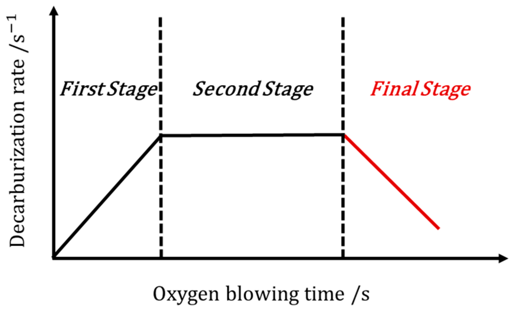
Figure 1.
The diagram of the decarbonization in the BOF process.
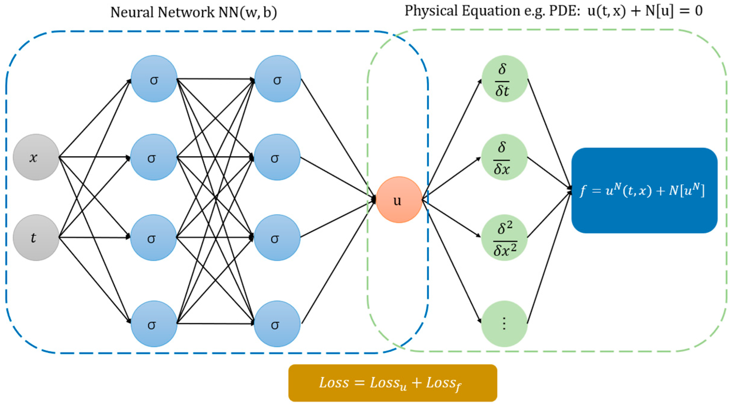
Figure 2.
A simple and classic structure of PINNs. The grey parts are neurons of the input layer of the neural network, the light-blue parts are neurons of the hidden layer, the orange part is neuron of the output layer, the green parts are differential results of automatic differentiation and the deep blue part is the residual error of the PDE.
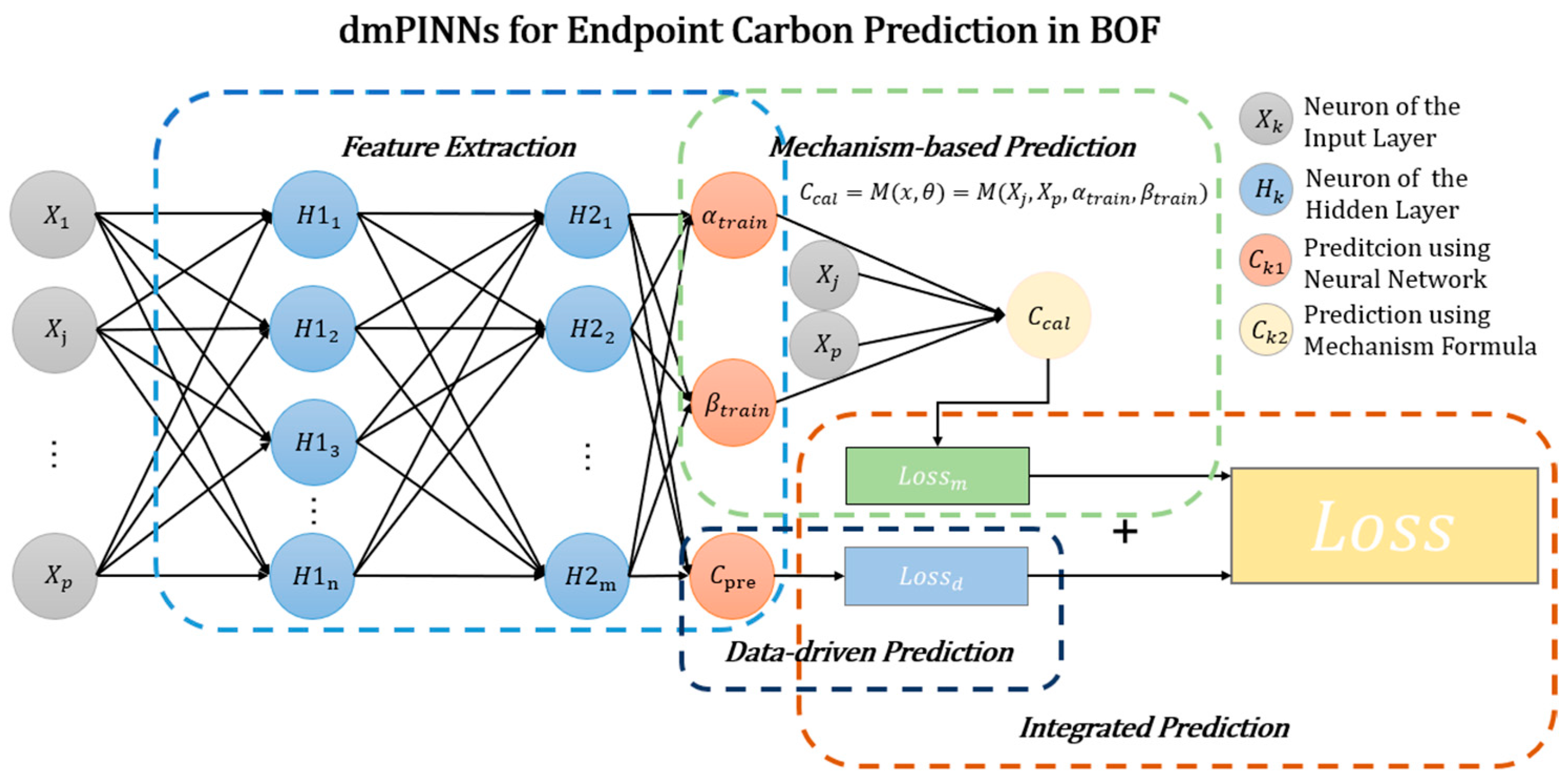
Figure 3.
Structure of dmPINNs. And , in the figure is Equation (5).
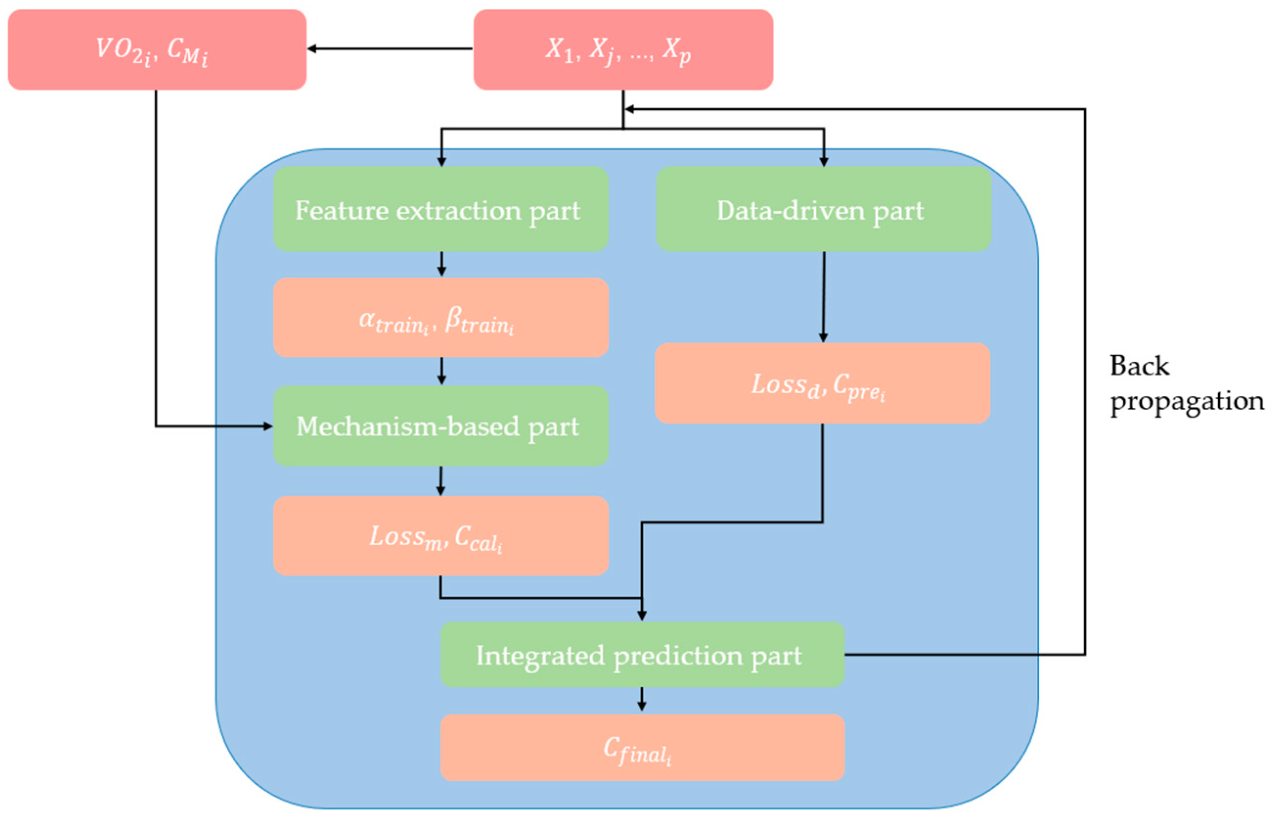
Figure 4.
The training flow chart of dmPINNs. The red parts are the input data, the orange parts are the process data or output data, the green parts are the four different parts of dmPINNs.
Figure 5.
Distribution of the prediction results of different parts of dmPINNs and the true value of endpoint carbon content.
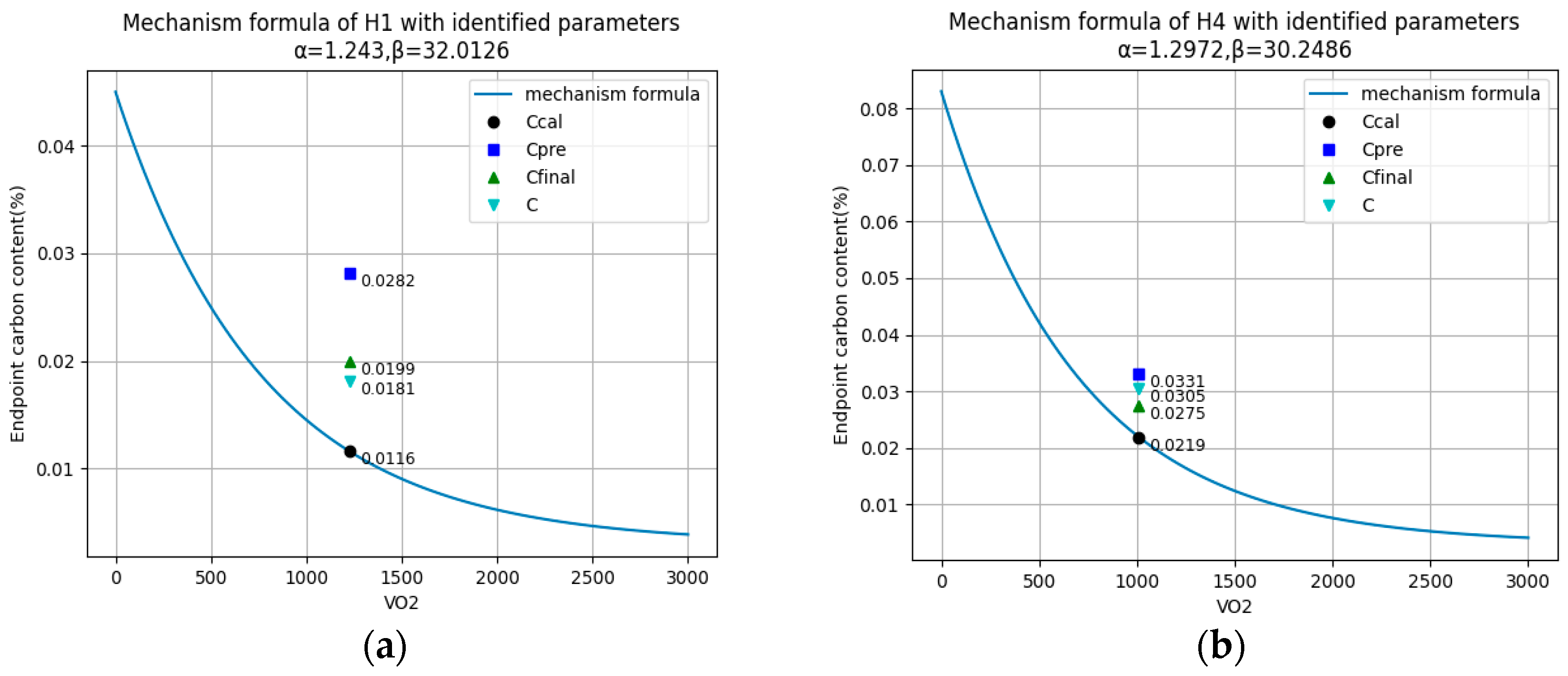
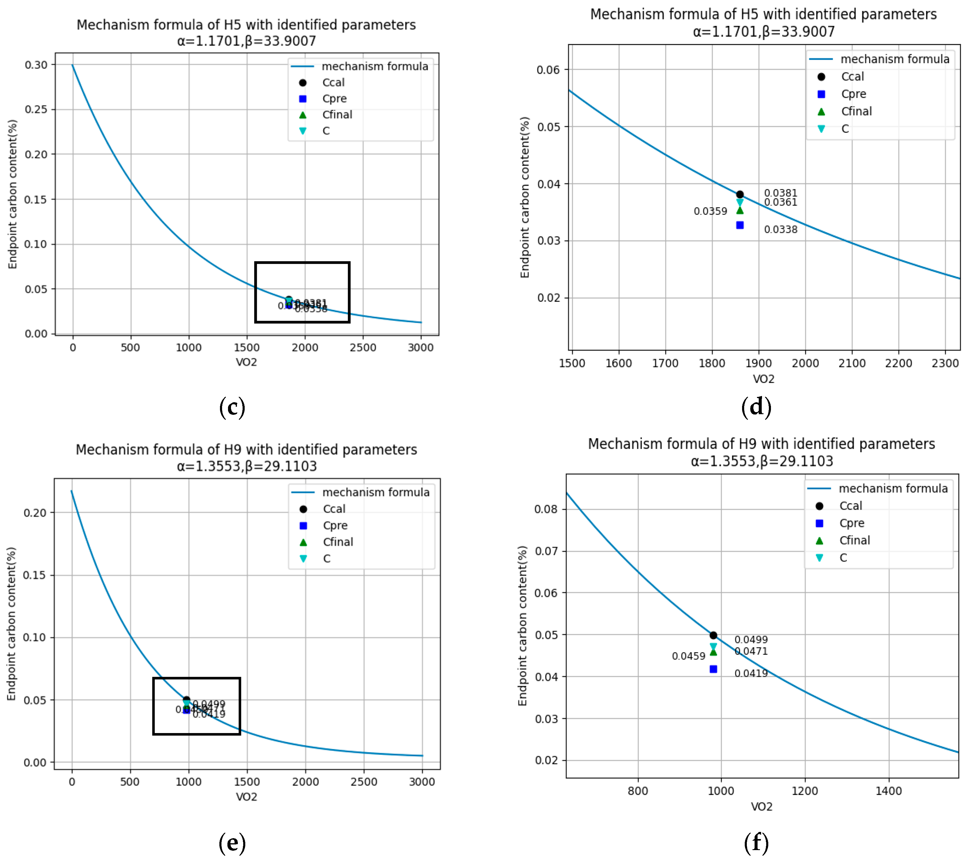
Figure 6.
Detailed prediction results of each part in dmPINNs. (a,b,c,e) are the complete prediction results of four heats. The two curves in panel (d) and panel (f) are the details of the rectangle at the left in (c,e).
Table 1.
Common nomenclature used in this paper.
| Nomenclature | Meaning |
|---|
| Oxygen consumption at the dynamic control stage |
| Critical carbon content (constant) |
| TSC carbon content |
| Weight of molten steel |
| of decarbonization mechanism formula |
| of decarbonization mechanism formula |
| of the formula identified by the feature extraction part |
| of the formula identified by the feature extraction part |
| Neuron of the input layer or influencing factor n |
| Neuron of the hidden layer |
| Hm | heat number m |
| Endpoint carbon content directly predicted by data-driven part in dmPINNs |
| Endpoint carbon content calculated by mechanism-based part in dmPINNs |
| Final endpoint carbon content in dmPINNs |
| True value of endpoint carbon content |
| Loss of the data-driven part of dmPINNs |
| Loss of the mechanism-based part of dmPINNs |
| is predicted based on the i-th heat of training data |
Table 2.
The training process description of dmPINNs.
| Training Process Description |
|---|
| 1. Input the heat data , , …, into dmPINNs, which contain the feature extraction part, the mechanism-based part, the data-driven part and the integrated prediction part. |
| 2. In the feature extraction part, features of the data are extracted, and they are used to identify the unmeasurable parameters , for each heat. |
| 3. In the data-driven part, is predicted directly and is calculated. |
| 4. In the mechanism-based part, mechanism formula is obtained for each heat through , , , , and then is calculated and is calculated. |
| 5. In the integrated prediction part, the total loss is designed as the sum of and , and the final prediction result is calculated through the weighted sum of and . |
| 6. Backpropagate and update parameters of the network, then go to (2). |
Table 3.
Statistical results of influencing factors.
| Influence Factors | Units | Symbols | Mean. |
|---|
| Weight of hot metal | t | | 268.29 |
| Weight of pure metals in scrap | t | | 51.027 |
| Weight of scrap | t | | 53.626 |
| Weight of heat-generating Agent A | t | | 1.4799 |
| Weight of flux A (CaO) | t | | 10.0674 |
| Weight of flux B | t | | 1.4333 |
| Weight of flux C | t | | 4.7906 |
| in hot metal | % | | 4.6121 |
| in hot metal | % | | 0.3642 |
| in hot metal | % | | 0.2046 |
| in hot metal | % | | 0.01027 |
| in hot metal | % | | 0.00132 |
| Oxygen consumption before TSC | | | 12,688.9 |
| Total oxygen consumption | | | 14,151.5 |
| °C | | 1614.9 |
| % | | 0.2415 |
| % | TSOC | 0.03886 |
Table 4.
Hit rate of different prediction methods.
| Methods | Hit Rate (%) |
|---|
| ±0.009 (%) 1 | ±0.012 (%) | ±0.02 (%) |
|---|
| BPNN | 63.00 | 76.14 | 92.48 |
| dmPINNs | 69.80 | 81.37 | 93.52 |
| dmPINNs_cal 2 | 69.45 | 80.00 | 93.35 |
| dmPINNs_pre | 66.67 | 78.63 | 93.85 |
Table 5.
Hit rate and the degradation of hit rate of different methods with the addition of noise.
| Methods | Hit Rate and Degradation of Hit Rate (%) |
|---|
| ±0.009 (%) 1 | ±0.012 (%) | ±0.02 (%) |
|---|
| Hit Rate | Degradation | Hit Rate | Degradation | Hit Rate | Degradation |
|---|
| BPNN | 63.00 | 0.00 | 76.14 | 0.00 | 92.48 | 0.00 |
| BPNN + 10%Noise | 62.45 | −0.55 | 74.83 | −1.31 | 91.50 | −0.98 |
| BPNN + 20%Noise | 61.96 | −1.04 | 75.81 | −0.33 | 92.15 | −0.33 |
| dmPINNs | 69.80 | 0.00 | 81.37 | 0.00 | 93.52 | 0.00 |
| dmPINNs + 10%Noise | 69.73 | −0.07 | 81.30 | −0.07 | 93.46 | −0.06 |
| dmPINNs + 20%Noise | 69.70 | −0.10 | 81.20 | −0.17 | 93.43 | −0.09 |
Table 6.
Prediction result of representative heats.
| Heat Number | () | (%) | () | | (%) | (%) | (%) | (%) |
|---|
| H1 | 1230 | 0.0450 | 1.2430 | 32.0126 | 0.0116 | 0.0282 | 0.0199 | 0.0181 |
| H2 | 1290 | 0.2060 | 1.2889 | 30.7900 | 0.0367 | 0.0329 | 0.0348 | 0.0382 |
| H3 | 1200 | 0.3630 | 1.4623 | 26.9789 | 0.0444 | 0.0539 | 0.0491 | 0.0538 |
| H4 | 1010 | 0.0830 | 1.2972 | 30.2486 | 0.0219 | 0.0331 | 0.0275 | 0.0305 |
| H5 | 1860 | 0.2990 | 1.1701 | 33.9007 | 0.0380 | 0.0338 | 0.0359 | 0.0361 |
| H6 | 1220 | 0.1760 | 1.2719 | 31.5642 | 0.0367 | 0.0373 | 0.0370 | 0.0369 |
| H7 | 430 | 0.0450 | 1.4671 | 26.7064 | 0.0221 | 0.0315 | 0.0268 | 0.0223 |
| H8 | 1340 | 0.2340 | 1.3233 | 29.7347 | 0.0348 | 0.0326 | 0.0337 | 0.0414 |
| H9 | 980 | 0.2170 | 1.3553 | 29.1103 | 0.0499 | 0.0419 | 0.0459 | 0.0471 |
| H10 | 1699 | 0.1760 | 1.1698 | 33.8685 | 0.0275 | 0.0307 | 0.0291 | 0.0275 |
Table 7.
Parameters and values of Heat H6.
| () | (%) | () | | (%) | (%) | (%) |
|---|
| 1220 | 0.1760 | 1.2719 | 31.5642 | 0.0373 | 0.0367 | 0.0370 |
Table 8.
Hit rate on the data of different steelmaking plants.
| Methods | Hit Rate (%) |
|---|
| ±0.009 (%) 1 | ±0.012 (%) | ±0.02 (%) |
|---|
| BPNN_S 2 | 63.00 | 76.14 | 92.48 |
| dmPINNs_S | 69.80 | 81.37 | 93.52 |
| BPNN_T | 82.67 | 92.15 | 97.38 |
| dmPINNs_T | 85.29 | 93.79 | 97.38 |
| Disclaimer/Publisher’s Note: The statements, opinions and data contained in all publications are solely those of the individual author(s) and contributor(s) and not of MDPI and/or the editor(s). MDPI and/or the editor(s) disclaim responsibility for any injury to people or property resulting from any ideas, methods, instructions or products referred to in the content. |
© 2024 by the authors. Licensee MDPI, Basel, Switzerland. This article is an open access article distributed under the terms and conditions of the Creative Commons Attribution (CC BY) license (https://creativecommons.org/licenses/by/4.0/).


