Galvanic Corrosion of E690 Offshore Platform Steel in a Simulated Marine Thermocline

Abstract

Marked changes in temperature, pH, dissolved oxygen (DO) content, and nutrient content typically occur in marine thermoclines, which are key factors that affect the corrosion of metals. Offshore platforms require marine metals to be exposed to deep-sea environments and thus increase their penetration into the marine thermocline. This study investigates the galvanic corrosion of E690 steel in a marine thermocline using a simulated marine thermocline (SMT). Specifically, the corrosion of E690 steel was analyzed using the wire beam electrode (WBE) technique, linear polarization (LP), corrosion morphology, and weight loss measurement. Results indicated that the SMT had a stable multilayer structure, and the variations in temperature, DO, pH, and nutrient concentration in the SMT were similar to those in the natural marine thermocline. There were two forms of E690 steel corrosion in the SMT: galvanic corrosion and seawater corrosion. The corrosion rate of seawater corrosion was influenced by the DO concentration. Galvanic corrosion occurred after the intrusion of E690 steel into the marine thermocline. The driver of galvanic corrosion was the difference values for E_corrs of E690 steel at various depths of the marine thermocline. The E_corr of E690 steel was influenced by the temperature, pH, and DO of the seawater, in the following order: DO >> T > pH. The continuous reduction in E_corr with depth contributed to large-scale galvanic corrosion, and the oscillation variation in E_corr with depth was the reason for small-scale galvanic corrosion. The primary anodic regions of galvanic corrosion were located in the area with the fastest temperature variation in the thermocline, and the position of the anodic regions rose with time. The anodic regions gradually expanded with time. The proportion of galvanic corrosion in the average corrosion rate could increase up to approximately 80% in the stable anodic region. There were many hemispherical corrosion pits on the surface of the single electrodes that were at the depths of 75 cm, 105 cm, and 135 cm. These single electrodes comprised a long-term, sustainable anodic region of galvanic corrosion.

1. Introduction

A basic three-layered structure (mixed layer, thermocline, and abyssal layer) is typical of low- and mid-latitude seawater [1,2]. Marine thermoclines are located at a water depth of nearly 30–150 m and exist all year round in tropical and subtropical oceans [3,4]. A marine thermocline is characterized by features of high hydrostatic pressure and dramatic changes in the concentrations of DO, hydrogen ions (pH), and nutrients. The trend of marine resource development is to explore and extract resources from deeper water [5,6]. Offshore platforms are the most important devices in marine resource exploitation [7,8]. E690 steel is a new type of high-strength low-alloy bainite steel [9] that has good comprehensive mechanical properties and high application potential in marine engineering structures [10,11,12]. Many studies have been conducted on the corrosion fatigue and SCC (stress corrosion cracking) of E690 in a simulated marine environment [13,14]. E690 steel (Nanjingsteel, Nanjing, China) has high SCC susceptibility in marine environments due to the combined mechanism of AD (anodic dissolution) and HE (hydrogen embrittlement) [15]. Ma et al. [16,17,18] reported that SO₂ in the marine atmosphere can facilitate the formation of a compact rust layer on the E690 steel surface, promoting the initiation of corrosion pits and reducing the toughness, and resulting in an increase in SCC susceptibility. Ma et al. [19] showed that the SCC susceptibility of E690 steel in simulated seawater was the lowest at approximately −850 mV/SCE and increased drastically when the potential was more negative than −950 mV/SCE. Although many studies have been performed on the corrosion of E690 steel in marine environments, most have focused on SCC and corrosion fatigue. Due to the influence of DO, water temperature, salinity, pH, and dissolved inorganic nitrogen [20,21,22,23,24,25], the corrosion process of steel is complex in marine environments. The corrosion mass loss of steel is promoted with the increase in dissolved oxygen concentration. In the main corrosion products of steel, the content of α-FeOOH is increased, while that of Fe₆(OH)₁₂CO₃ is decreased with increasing concentrations of dissolved oxygen. Differences in the characteristics of corrosion products can affect the corrosion resistance of the steel. A great number of cracks existing in the corrosion products of steel under the condition of pH = 7 result in severe corrosion. In contrast, the compactness of corrosion products is conducive to protecting the steel substrate at a pH of 9. Bacterial metabolism is influenced by the rate of the supply of critical nutrients (such as dissolved inorganic nitrogen). Under suitable conditions, the rate of the corrosion of steel is controlled by the rate of bacterial metabolism. The corrosion of E690 steel is still not fully understood in seawater, particularly in marine thermocline conditions.

With the progression of marine resource development, offshore platforms were built in “shallow water areas” for “deep water areas” [26]. The steel piles of offshore platforms are more likely to suffer longitudinal non-uniform corrosion in thermoclines. The factors effecting corrosion and the corrosion mechanism of steel piles (E690 steel) are inconclusive, which might compromise the security of offshore platforms. The non-uniform corrosion of E690 steel in a marine thermocline is investigated in this study. For this, a marine thermocline simulator (MTS) was designed and fabricated according to the formation mechanism of marine thermoclines. Seawater taken from the South China Sea served as the electrolyte for the creation of an SMT. Removable and chain-type wire beam electrodes (RCWBEs) were used to understand the corrosion of the steel specimen. Electrochemical measurements (galvanic corrosion measurement technology, linear polarization), corrosion morphology observations, and weight loss measurements were used to investigate the corrosion mechanism of E690 steel in the SMT.

2. Experiment

2.1. Simulated Marine Thermocline

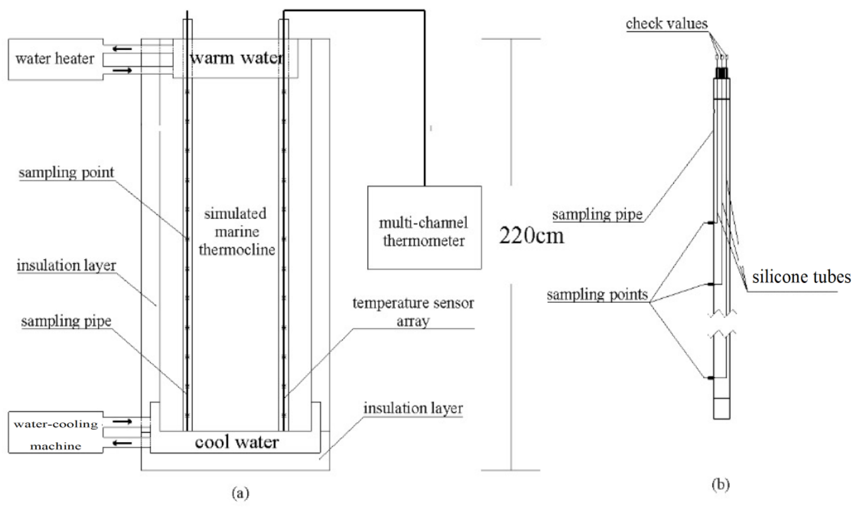
2.1.1. Marine Thermocline Simulator

Figure 1a shows a cross-section of the marine thermocline simulator (MTS). The MTS primarily included four parts: a heat preservation bucket, a temperature control unit, a temperature measurement unit, and a sampling tube. The temperature control unit contained a water heater, a water-cooling machine, a warm water tank, and a cool water tank. The warm water tank was fixed at the top of the MTS, which was used to keep the upper part of the SMT at a relatively high temperature. The cool water tank was fixed at the bottom of the MTS, which was used to keep the lower part of the SMT at a relatively low temperature. The temperature measurement unit contained a multichannel thermometer and a temperature sensor array. Figure 1b shows a cross-section of the sampling tube, which was used to take seawater samples for analysis.

Figure 1. Cross-section image of the marine thermocline simulator: (a) cross-section of the MTS; (b) cross-section of the sampling tube.

2.1.2. Measurement of Marine Thermocline Parameters

Seawater taken from the South China Sea served as the electrolyte for the SMT. The seawater was added to the heat preservation bucket before the MTS was operated.

• Temperature measurement
  The temperature measurement unit contained a multichannel thermometer and temperature sensor array. The temperature sensors were numbered 1 to 12 from the bottom to the top. The temperature data were collected every 10 min.
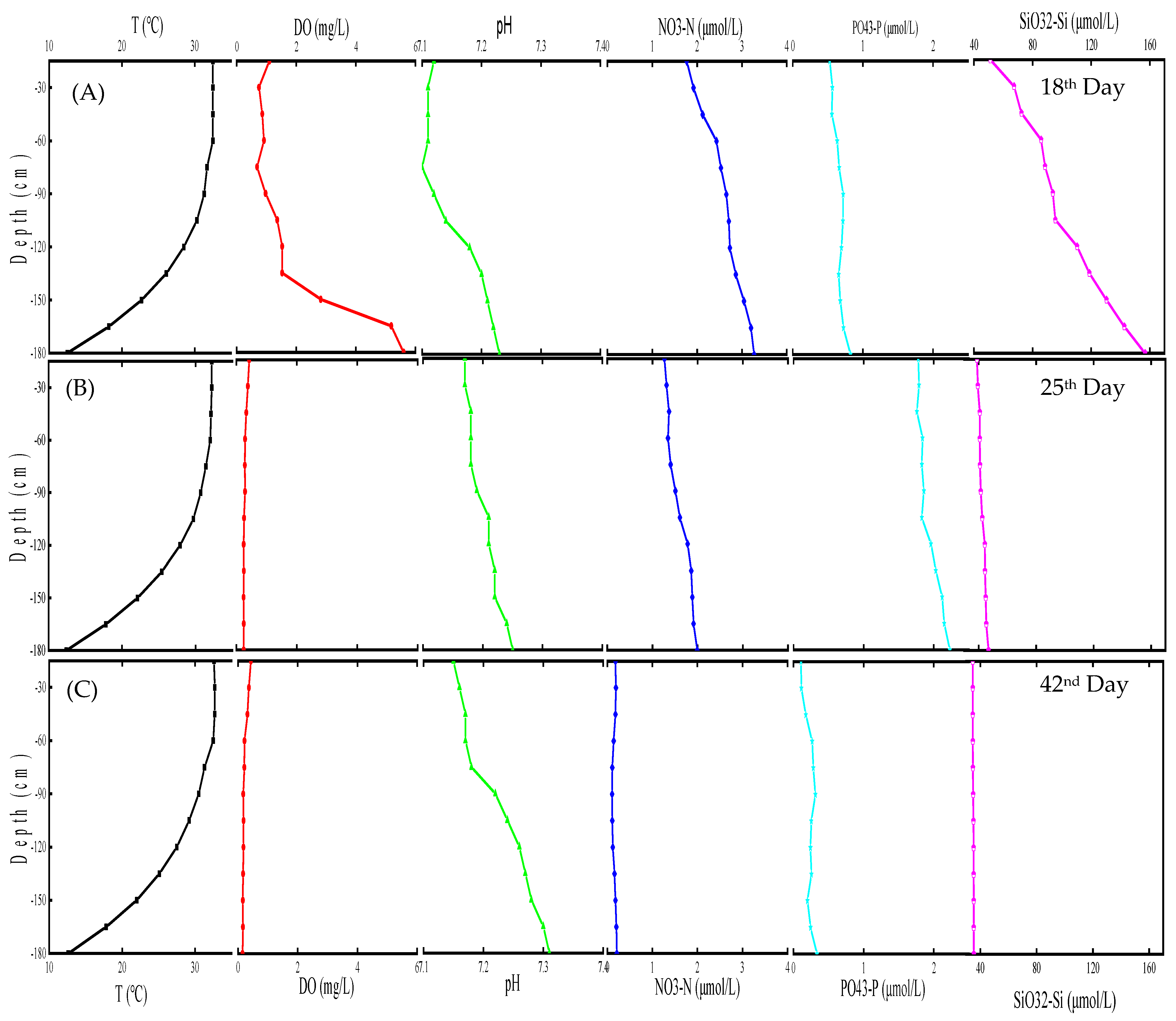
• pH measurement
  The SMT lasted for 66 days. On the 18th, 25th, and 42nd days, seawater samples were taken through the sampling tube. The seawater sample’s pH was measured immediately by a pH meter with temperature compensation.
• Measurement of DO and nutrient contents
  The DO and nutrient (nitrate, phosphate, and silicate) contents of the seawater samples were determined using a chemical method [27] on the 18th, 25th, and 42nd days. The Wenkler method was employed for the analytical determination of DO in seawater. The method utilized for the analysis of nitrate in the seawater involved zinc sheet reduction followed by neethylenediamine spectrophotometry. The analyses of both the phosphates and silicates were conducted using molybdate amine chromogenic spectrophotometry.

2.2. Material

The E690 steel used in this study was produced by China Baowu Steel Group Corporation Limited (Shanghai, China), and its microstructure was lath-like bainite. The chemical composition of the E690 steel is shown in Table 1. The E690 steel was cut into specimens, which were 4 mm thick and 39 mm diameter discs. The specimens were gradually ground down to 1000 grid with SiC paper, degreased with acetone, and rinsed with deionized water.

Removable and-chain-type wire beam electrodes (RCWBEs) [28] were used to understand the corrosion of the steel specimen with the aid of the wire beam electrode (WBE) technique. The RCWBEs were used to simulate the long metal in the SMT and consisted of many individual electrodes with an adjacent separation of 15 cm. The individual electrode was fabricated from an E690 steel specimen, rubber ring, PVC screw, and wires. Figure 2a,b show the two types of RCWBE in response to different purposes: “A”, used for electrochemical measurements, and “B”, used for morphological observation and corrosion weight loss rate measurements.

Figure 2. Connection model of RCWBEs: (a) for electrochemical measurements; (b) for morphological observation and corrosion weight loss rate measurements. There are 13 single electrodes, the * is ellipsis to reduced graphs.

Table 1. Chemical composition of E690 steel, in wt.%.

C	Si	Mn	P	S	Cr	Ni	Cu	Mo	V	Als	Fe
0.15	0.20	1.00	0.0058	0.0014	0.99	1.45	0.0091	0.37	0.03	0.036	Bal.

Table 1. Chemical composition of E690 steel, in wt.%.

C	Si	Mn	P	S	Cr	Ni	Cu	Mo	V	Als	Fe
0.15	0.20	1.00	0.0058	0.0014	0.99	1.45	0.0091	0.37	0.03	0.036	Bal.

2.3. Corrosion Research Method

The RCWBEs were vertically placed in the SMT, where the bottom single electrodes were 10 cm above the bottom section. The single electrode and corresponding temperature measurement point and corresponding sampling point were located at the same cylindrical surface.

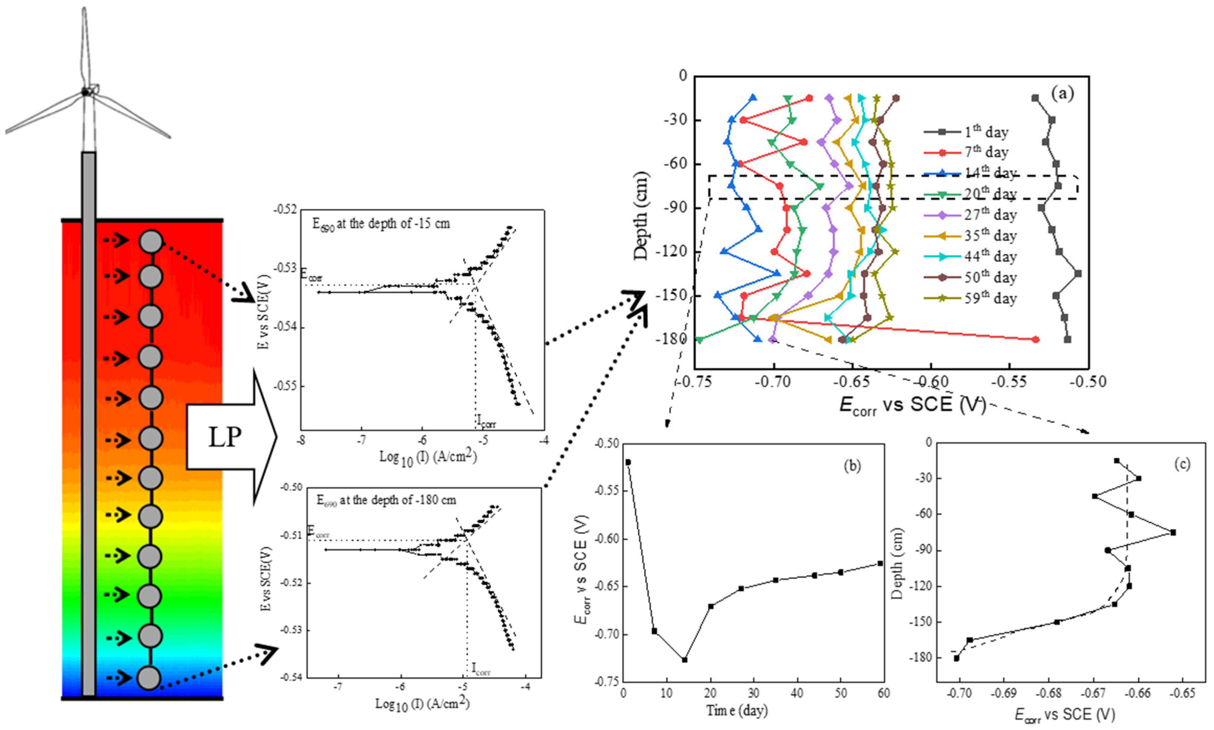
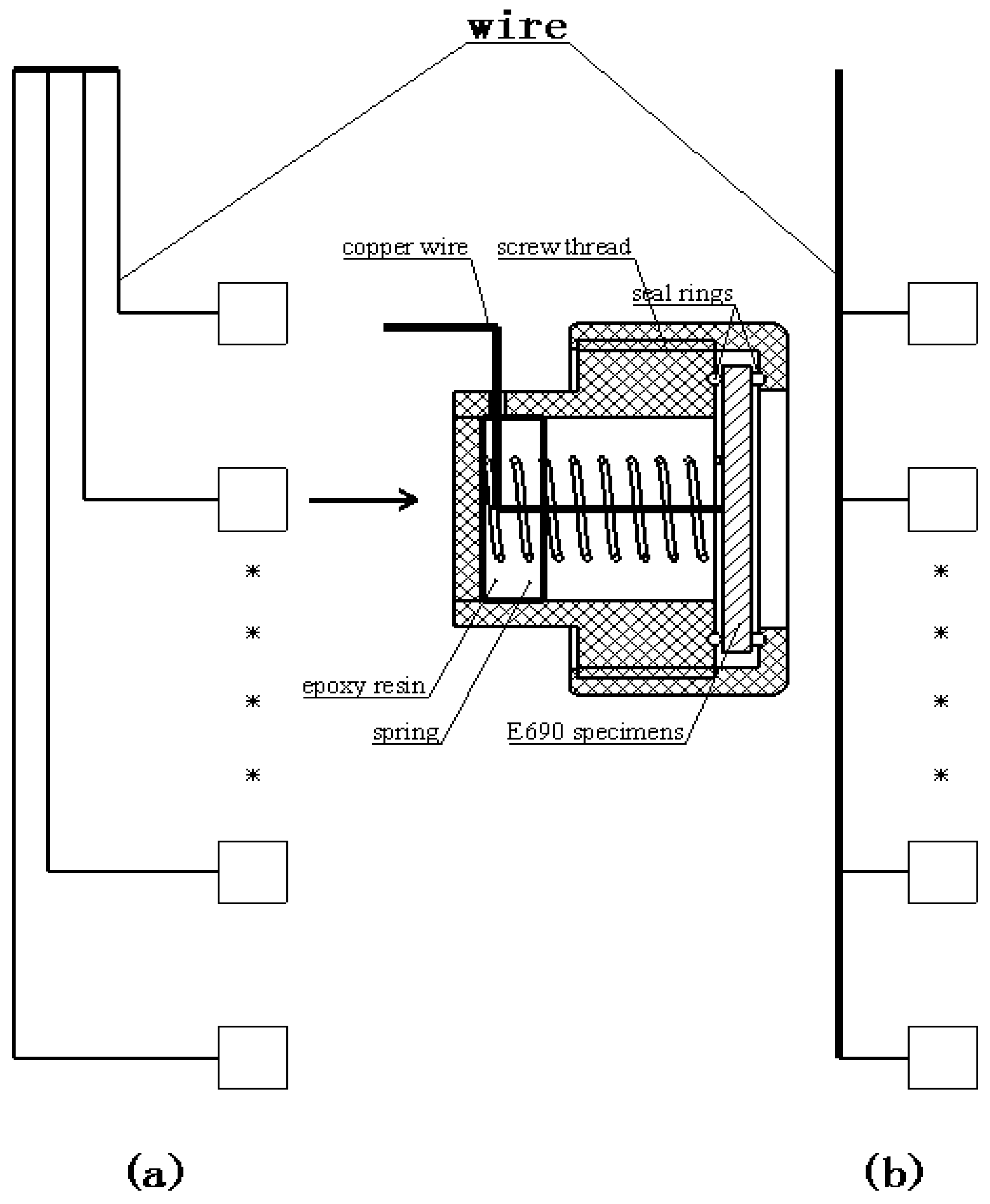
2.3.1. Measurement of RCWBE Galvanic Currents

In situ measurements of the galvanic currents were performed on the 1st, 7th, 14th, 20th, 27th, 44th, and 59th days. Galvanic currents of the RCWBEs were measured using the electrochemical noise (ECN) method via a PGSTAT302N AUTOLAB (Metrohm AG, Herisau, Switzerland) potentiostat and NOVA1.11 software. Two working electrodes (W1, W2) and one reference electrode, the saturated calomel electrode (SCE), were considered for the ECN measurement. A single electrode of one column of RCWBEs was connected with W1, while the other electrodes of the same column were simultaneously connected with W2. The ECN of every single electrode was measured for 30 s, and then the electrodes connected with W1 and W2 were replaced. Then, the ECN of the entire RCWBE column was measured, and the galvanic current of each electrode of the array was determined from the analyzed ECN data [28,29].

2.3.2. Measurement of Instantaneous I_corr and E_corr

In situ measurements for linear polarization (LP) were performed on the 1st, 7th, 14th, 20th, 27th, 44th, and 59th days. The single electrodes were each subjected to LP on a three-electrode cell, which comprised a single electrode as the working electrode, a 2 × 2 cm² Pt plate as the counter electrode, and an SCE as the reference electrode. The LP curves were measured via potential scanning from −10 to +10 mV against open-circuit potentials at a rate of 0.00167 mV/s. Instantaneous values of each electrode I_corr and E_corr were obtained from analysis of the LP data.

2.3.3. Corrosion Morphology Observation

The B-type RCWBEs were removed from the MTS on the 10th, 23rd, 32nd, 41st, 51st, and 66th days, and then observed via a HITACHI TM4000 Plus SEM (Hitachi High-Tech Corporation, Tokyo, Japan) three-dimensional microscope and camera. After derusting and drying, each electrode was observed again.

2.3.4. Weight Loss Measurement

Pre-weighed E690 steel specimens were installed in the B-type RCWBEs and then immersed in the simulated thermocline. After morphological observation of the specimens, they were cleaned with acetone and reweighed. The weight loss data were calculated using the formula given in Equation (1):

$$V(\mathrm{mm}/\mathrm{y})=8760(\mathrm{h}/\mathrm{y})\times 10(\mathrm{mm}/\mathrm{cm})\times \frac{W_0(\mathrm{g})-W_1(\mathrm{g})}{\rho ({\mathrm{g}/\mathrm{cm}}^3)\cdot A({\mathrm{cm}}^2)\cdot t(\mathrm{h})}$$

(1)

where V is the average corrosion rate, in mm/y; W₀ is the initial weight of the E690 specimen, in g; W₁ is the weight of the derusted E690 specimen, in g; A is the exposure area of the E690 specimen, in cm²; t is the exposure time, in hours; and ρ is the density of the metal, in g/cm³.

3. Results and Discussion

3.1. Characterization of the Simulated Marine Thermocline

The temperature measurement points and sampling points were numbered 1 to 12 from bottom to top, respectively. Seawater at room temperature was added to the heat preservation bucket before the MTS was operated. The entire experiment lasted for 66 days, and the temperature data were collected every 10 min. On the 18th, 25th, and 42nd days, seawater samples at different depths were removed through the sampling pipe, and their pH, DO, and nutrient content were measured.

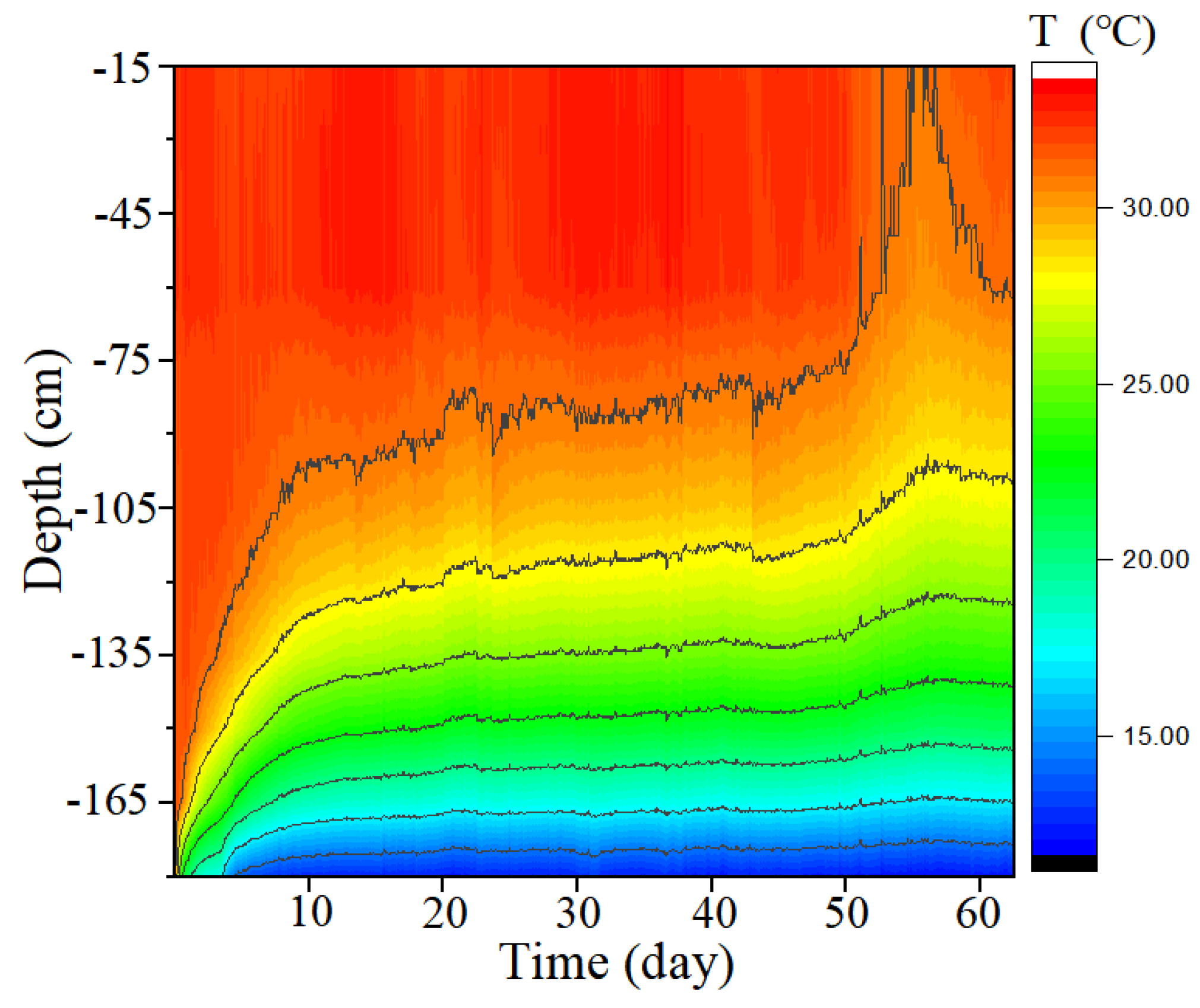
3.1.1. Temperature Variation in the Simulated Marine Thermocline

Figure 3 shows the longitudinal temperature variation in the SMT. From day 0 to the 7th day, the temperature at the bottom points changed markedly. A stable and strong temperature gradient first appeared on the 7th day and lasted until the 66th day. After the 7th day, the multilayer structure of seawater formed and remained stable. The temperature of the upper seawater layer was 32 °C, and that of the lower seawater layer was 12 °C. The range of temperature variation in the SMT was similar to that in the marine thermocline in the northern area of the South China Sea (NSCS) in summer. In summer, the surface temperature increases from northeast to southwest, ranging from 28.2 to 30.7 °C in the NSCS. In summer, the average upper to lower boundary depth of the thermocline in the NSCS is about 18–56 m (thickness: 38 m) on the shelf and 32–129 m (thickness: 97 m) beyond the shelf; the temperature gradient in our simulated thermocline was 0.21 °C m⁻¹ on the shelf and 0.12 °C m⁻¹ beyond the shelf [30]. The thermal distribution of the thermocline in the NSCS beyond the shelf was thus simulated using the SMT.

Figure 3. Longitudinal variation with time of temperature in the simulated marine thermocline.

3.1.2. Component Variation in the Simulated Marine Thermocline

Figure 4 shows the component variations in the SMT. On the 18th day, the DO increased with increasing seawater depth. The DO of the upper-layer seawater decreased from 1.09 mg/L on the 18th day to 0.42 mg/L on the 25th day. The DO of the bottom seawater decreased from 5.60 mg/L to 0.24 mg/L. The DO decreased with increasing seawater depth on the 25th and 42nd days. The variation in DO in the SMT showed a stable multilayer structure formation. There is a small quantity of biodetritus in natural seawater. As shown in Reaction (2), the biodetritus slowly decomposed into inorganic substances and simultaneously consumed the DO. The decomposition reaction of biodetritus is influenced by temperature. Before the 18th day, the DO consumption rate in the warm and upper seawater was higher than that in the cool and bottom seawater. The O₂ transmission is subject to the stable multilayer structure of the thermocline:

$${(C{H}_{2}O)}_{106}{(N{H}_3)}_{16}{H}_{3}P{O}_4+138O_2\to 106C{O}_2+16{HNO}_3+H_3{PO}_4+122H_{2}O$$

(2)

Figure 4. Evolution of simulated marine thermocline structure: (A) 18th day; (B) 25th day; (C) 42nd day.

The seawater pH increased with increasing seawater depth and decreased with time. As seen in Reaction (3), CO₂ and H⁺ were produced in the biodetritus decomposition process. The decomposition rate of biodetritus in the warm and upper seawater was higher than that in the cool and bottom seawater:

$$(C{H}_{2}O{)}_{106}{(N{H}_3)}_{16}{H}_{3}P{O}_4+84.8HN{O}_3\to 106C{O}_2+42.4N_2+6N{H}_3+H_{3}P{O}_4+148.4H_{2}O$$

(3)

Reaction (2) shows the decomposition reaction of biodetritus in oxygen-enriched seawater, and Reaction (3) shows that in oxygen-poor seawater. Biodetritus decomposition caused the nitrate concentration in the initial and high-DO stages of the thermocline to increase. With dwindling DO levels, the nitrate concentration decreased for the biodetritus decomposition, as seen in Reaction (3). The concentration changes of phosphate and silicate were influenced by the biodetritus decomposition and pH variation.

Considering all of these results, the SMT was a stable multilayer structure, and the variation trends of the temperature, DO, pH, and nutrient concentration in the SMT were similar to those in a natural marine thermocline.

3.2. Galvanic Corrosion of E690 Offshore Platform Steel in a Simulated Marine Thermocline

Figure 5 shows the variation in the galvanic current (I_G) of WBEs in the SMT. The maximum I_G increased with the experiment’s duration from the 7th day to the 44th day. The maximum I_G of the galvanic anode increased from −3 μA/cm² on the 7th day to −12 μA/cm² on the 44th day. The maximum I_G of the galvanic cathode increased from 3.5 μA/cm² on the 7th day to 27.5 μA/cm² on the 44th day. The maximum I_G of both the galvanic cathode and anode decreased on the 59th day. The maximum I_G of the galvanic anode decreased from −12 μA/cm² on the 44th day to −4.5 μA/cm² on the 59th day, and then, the maximum I_G of the galvanic cathode decreased from 27.5 μA/cm² on the 44th day to 18 μA/cm² on the 59th day. From the longitudinal temperature variation in the SMT, the primary anodic regions were located in the fastest temperature variation area, and the position of the primary anodic region rose with time. From the 7th day to the 44th day, the anodic regions gradually expanded. The anodic region was intermixed with the cathodic region on the 59th day and in the lower part of the SMT.

Figure 5. Variation in galvanic current of RCWBEs in the SMT. The arrow and dashed lines told the readers that the position of the primary anodic region rose with time.

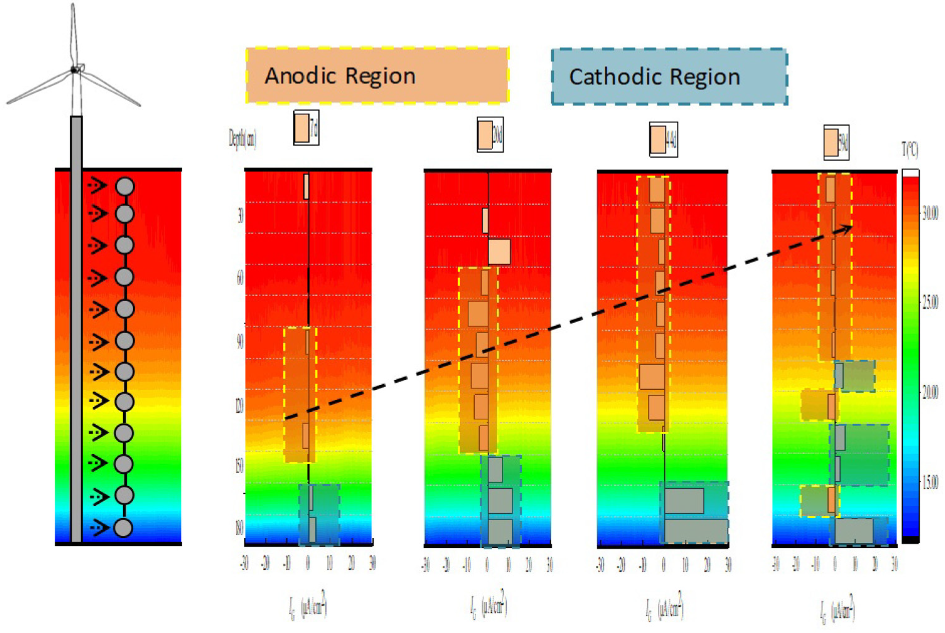
3.3. Driver of E690 Offshore Platform Steel Galvanic Corrosion in the SMT

The E_corr values of single electrodes were measured using in situ linear polarization measurements. Figure 6a describes all E_corr values of the E690 steel in the simulated thermocline. The E_corr of a single electrode at a depth of 75 cm changed with time, as shown in Figure 6b. The E_corr markedly decreased from −0.519 V vs. SCE on the 1st day to −0.727 V on the 14th day and then gradually increased with time. The electrochemical corrosion reaction of steel (see Reactions (3)–(5)) and the Nernst equation (see Equation (7)) showed that the E_corr of the steel was influenced by the temperature, pH, and DO of the seawater. Comparing the E_corr variation and marine thermocline component variation, E_corr was most affected by the DO. DO is a crucial factor that affects the corrosion behavior of alloys. DO can be used as a cathode depolarizer, while it also has a tendency to passivate the metal surface. This result was supported by the macrocorrosion morphology of the rusted E690 specimens (see Table 2). Due to the high concentration of DO, the color of the E690 corrosion products was yellowish on the 7th day (i.e., the principle in Reaction (6)). The color of the E690 corrosion products changed from yellowish high-valence iron compounds to taupe low-valence iron compounds with time and depth. For the small variation in pH in the simulated thermocline, the E_corr was marginally affected by pH. The E_corr of E690 steel was influenced by the temperature, pH, and DO of the seawater in the simulated thermocline in the following order: DO >> T > pH.

Table 2. Macrocorrosion morphology of rusted E690 specimens in the simulated thermocline.

Depth (cm)	Time
	7th Day	20th Day	27th Day	44th Day	59th Day
15
45
75
105
135
165
180

If a lengthy steel structure traverses the marine thermocline, the galvanic corrosion of steel is primarily driven by variations in its electrochemical potential at different depths. As shown in Figure 6c, the continuous reduction in E_corr with depth contributed to large-scale galvanic corrosion, and the oscillation variation of E_corr with depth was the reason for small-scale galvanic corrosion:

Negative electrode reaction:

$$2Fe\to 2F{e}^{2+}+4e^{-}$$

(4)

Positive electrode reaction:

$$O_2+2H_{2}O+4e^{-}\to 4O{H}^{-}$$

(5)

Total reaction equation:

$$2Fe+O_2+2H_{2}O\to 2F{e}^{2+}+4O{H}^{-}$$

(6)

Oxygen-enriched seawater environment:

$$4Fe{(OH)}_2+O_2+2H_{2}O\to 4Fe{(OH)}_3$$

(7)

According to the Nernst equation:

$$E_{(F{e}^{2+}/Fe)}=E_{(F{e}^{2+}/Fe)}^{\mathrm{\Theta }}+\frac{RT}{nF}Ln\frac{p_{O_2}}{{(C_{F{e}^{2+}}/C_{F{e}^{2+}}^{\mathrm{\Theta }})}^2\cdot {(C_{O{H}^{-}}/C_{O{H}^{-}}^{\mathrm{\Theta }})}^4}$$

(8)

$E_{(F{e}^{2+}/Fe)}$: real electrode potential; $E_{(F{e}^{2+}/Fe)}^{\mathrm{\Theta }}$: standard electrode potential;

$n$: the number of transferred electrons in the reaction equation;

$F$: Faraday’s constant (96,485 C·mol⁻¹); $R$: gas constant (8.314 J·K⁻¹mol⁻¹);

$T$: temperature (K); $P_{O_2}$: partial pressure of O₂;

$C_x$: concentration of $x$ (mol·L⁻¹);

$C_x^{\mathrm{\Theta }}$: concentration of $x$ under normal conditions (mol·L⁻¹).

Figure 6. Variation in E690 steel Ecorr values in the simulated thermocline: (a) the E_corr variation in all specimens; (b) the E_corr variation for a single electrode at a depth of 75 cm; (c) the E_corr variation for a single electrode on the 27th day.

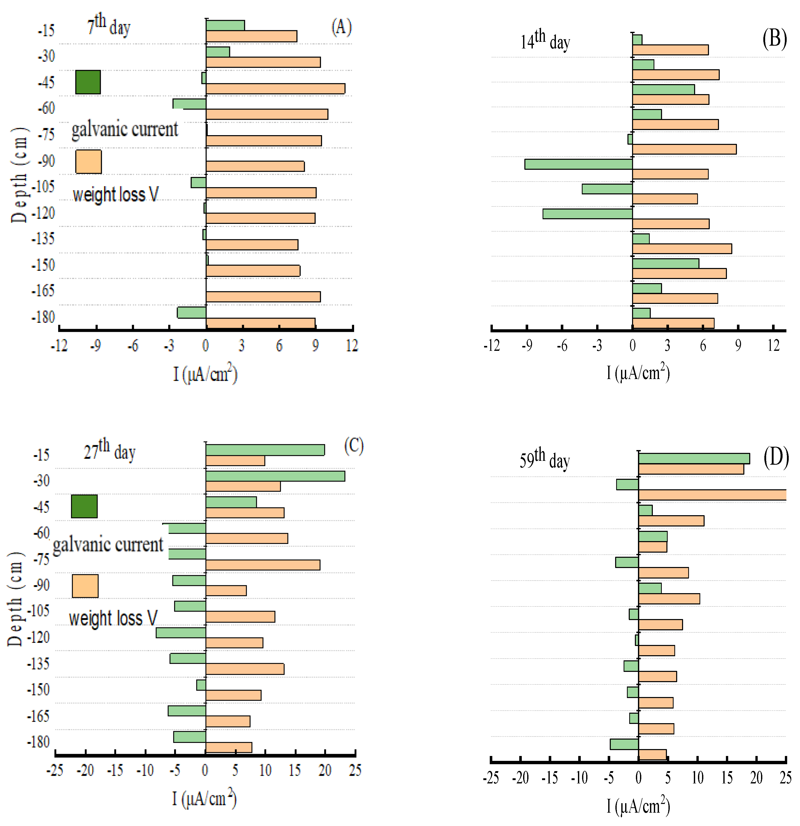
3.4. Proportion of Galvanic Corrosion in E690 Offshore Platform Steel Corrosion

The average corrosion rates of E690 steel at the various depths of the SMT were measured via weight loss measurement. The “mm/y” of the average corrosion rate unit was converted into “μA/cm²”. Figure 7 shows a comparison of the galvanic current and average corrosion rate (weight loss rate). There were two forms of E690 steel corrosion in the SMT: galvanic corrosion and seawater corrosion. The seawater corrosion was the primary contributor to the average corrosion. The seawater corrosion of the E690 steel was influenced by DO (i.e., the principle in Reactions (3)–(6)). Before the 7th day, there was enough DO in the thermocline to prevent the corrosion of E690. The average corrosion rates of the single electrodes were biggest. The DO variation in the seawater was small, and the longitudinal average corrosion rate variation in the single electrodes was small. With the decrease in DO content, the average corrosion rates of the single electrodes decreased after the 7th day. On the 14th day, a DO concentration gradient was established with the seawater depth (as Figure 4A); then, the value of the differences in the E_corrs of the single electrodes became bigger (as Figure 6a). The bigger difference values for the E_corrs of single electrodes led to a larger galvanic current on the 14th day. When galvanic corrosion was formed, the cathode potential moved to the negative potential, and anodic potential moved to the positive potential. The difference values for the E_corrs of the single electrodes then changed to small, which led to the galvanic current reducing on the 27th day and 59th day. This result was supported by the average corrosion rate variation in Figure 7, the quantity variation in corrosion products in Table 3, and the variation trends of the DO in Figure 4. In the anodic region of galvanic corrosion, the proportion of galvanic corrosion’s contribution to the average corrosion rate first increased and then decreased. The proportion of galvanic corrosion in the average corrosion rate could increase up to approximately 80% in the anodic region. As shown in Table 4, there were many hemispherical corrosion pits at the depths of 75 cm, 105 cm, and 135 cm. Hemispherical corrosion pits are typical of the morphology of anodic dissolution corrosion of steel. The single electrodes at the depths of 75 cm, 105 cm, and 135 cm represent a long-term, sustainable anodic region of galvanic corrosion.

Figure 7. Comparison of galvanic current and average corrosion rate: (A) the 7th day; (B) the 7th day; (C) the 27th day; (D) the 59th day.

Table 3. Microcorrosion morphology of rusted E690 specimens in the simulated thermocline (100×).

Depth (cm)	Time
	7th Day	20th Day	27th Day	44th Day	59th Day
15
45
75
105
135
165
180

Table 4. Microcorrosion morphology of derusted E690 specimens in the simulated thermocline (200×).

Depth (cm)	Time
	7th Day	20th Day	27th Day	44th Day	59th Day
15
45
75
105
135
165
180

4. Conclusions

Offshore platforms allow their seepage to develop in the deep sea, along with the penetration of a growing number of steel piles throughout marine thermoclines. To determine the scientific and practical value of galvanic corrosion in marine thermoclines, this study investigated the corrosion of E690 steel using a simulated seawater thermocline that was designed and fabricated using developed RCWBEs. The major findings of this first test study include the following:

(1)

The SMT showed a stable multilayer structure. The variations in temperature, DO, pH, and nutrient concentration in the SMT were similar to those seen in a natural marine thermocline.

(2)

Galvanic corrosion occurred after the intrusion of E690 steel into the marine thermocline. Primary anodic regions were located in the area with the fastest temperature variation, and the anodic regions were intermixed with the cathodic region in the lower part of the stable marine thermocline.

(3)

The driver of galvanic corrosion of E690 steel in the marine thermocline was the $\mathrm{\Delta }Ecorr$ of the E690 steel at various depths. The continuous reduction in E_corr with depth contributed to large-scale galvanic corrosion, and the oscillation variation of E_corr with depth was the reason for small-scale galvanic corrosion.

(4)

The E_corr values of the E690 steel were influenced by the temperature, pH, and DO in the marine thermocline, in the following order: DO >> T > pH.

(5)

There were at least two forms of E690 steel corrosion in the marine thermocline: galvanic corrosion and seawater corrosion. The proportion of galvanic corrosion in the average corrosion rate could increase up to approximately 80% in the anodic region. There were many deep corrosion pits in the long-term and stable anodic region of galvanic corrosion.

References

- Lynne, D.T.; Pickard, G.L. Typical Distributions of Water Characteristics. In Descriptive Physical Oceanography: An Introduction, 6th ed.; Elsevier: London, UK, 2011; pp. 67–110. [Google Scholar]
- Tang, Z.; Li, T. Remote and local controls on dissolved oxygen in the Western Tropical Pacific thermocline during the last 700 kyr. Palaeogeogr. Palaeocl. 2024, 638, 112015. [Google Scholar] [CrossRef]
- Zhang, M.; Shu, Q. Spatiotemporal propagating decadal signal of ocean heat content and thermocline depth identified in the tropical Pacific. Sci. Total Environ. 2022, 838, 155972. [Google Scholar] [CrossRef] [PubMed]
- Kang, M.; Oh, S. Acoustic characterization of fish and macroplankton communities in the Seychelles-Chagos thermocline ridge of the southwest Indian ocean. Deep-Sea Res. Part II 2024, 213, 105356. [Google Scholar] [CrossRef]
- Dehghani, A.; Aslani, F. A review on defects in steel offshore structures and developed strengthening techniques. Structures 2019, 20, 635–657. [Google Scholar] [CrossRef]
- Zheng, Z.; Chang, Z. Mitigating deepwater jacket offshore platform vibration under wave and earthquake loadings utilizing nonlinear energy sinks. Ocean Eng. 2023, 283, 115096. [Google Scholar] [CrossRef]
- Morales, Y.; Samanta, P. Water management for Power-to-X offshore platforms: An underestimated item. Sci. Rep. 2023, 13, 12286. [Google Scholar] [CrossRef] [PubMed]
- Ben, N.; Vytyaz, O.Y. Mechanical properties of steel for floating offshore platforms under static and cyclic loading. Mater. Sci. 2024, 59, 152–157. [Google Scholar] [CrossRef]
- Li, Y.; Liu, Z. Effect of cathodic potential on stress corrosion cracking behavior of different heat-affected zone microstructures of E690 steel in artificial seawater. J. Mater. Sci. Technol. 2021, 64, 141–152. [Google Scholar] [CrossRef]
- Liu, Z.; Hao, W. Fundamental investigation of stress corrosion cracking of E690 steel in simulated marine thin electrolyte layer. Corros. Sci. 2019, 148, 388–396. [Google Scholar] [CrossRef]
- Ma, H.C.; Fan, Y. Effect of pre-strain on the electrochemical and stress corrosion cracking behavior of E690 steel in simulated marine atmosphere. Ocean Eng. 2019, 182, 188–195. [Google Scholar] [CrossRef]
- Ma, H.C.; Liu, Z.Y. Stress corrosion cracking of E690 steel as a welded joint in a simulated marine atmosphere containing sulphur dioxide. Corros. Sci. 2015, 100, 627–641. [Google Scholar] [CrossRef]
- Lu, Q.; Wang, L. Corrosion evolution and stress corrosion cracking of E690 steel for marine construction in artificial seawater under potentiostatic anodic polarization. Constr. Build. Mater. 2020, 238, 117763. [Google Scholar] [CrossRef]
- Li, G.; Li, Y. Evaluation of the impact of chloride ion concentration on stress corrosion cracking in E690 steel under low pH conditions. Int. J. Electrochem. Sci. 2023, 18, 100375. [Google Scholar] [CrossRef]
- Tian, H.; Wang, X. Electrochemical corrosion, hydrogen permeation and stress corrosion cracking behavior of E690 steel in thiosulfate-containing artificial seawater. Corros. Sci. 2018, 144, 145–162. [Google Scholar] [CrossRef]
- Ma, H.; Liu, Z. Comparative study of the SCC behavior of E690 steel and simulated HAZ microstructures in a SO2-polluted marine atmosphere. Mater. Sci. Eng. A 2016, 650, 93–101. [Google Scholar] [CrossRef]
- Ma, H.; Du, C. Effect of SO2 content on SCC behavior of E690 high-strength steel in SO2-polluted marine atmosphere. Ocean Eng. 2018, 164, 256–262. [Google Scholar] [CrossRef]
- Ma, H.; Chen, L. Effect of prior austenite grain boundaries on corrosion fatigue behaviors of E690 high strength low alloy steel in simulated marine atmosphere. Mater. Sci. Eng. A 2020, 773, 138884. [Google Scholar] [CrossRef]
- Ma, H.; Liu, Z. Effect of cathodic potentials on the SCC behavior of E690 steel in simulated seawater. Mater. Sci. Eng. A 2015, 642, 22–31. [Google Scholar] [CrossRef]
- Gardiner, C.P.; Melchers, R.E. Corrosion analysis of bulk carriers, Part I: Operational parameters influencing corrosion rates. Mar. Struct. 2003, 16, 547–566. [Google Scholar] [CrossRef]
- Wei, H.; Tang, Y. Corrosion behavior and microstructure analysis of butt welds of Q690 high strength steel in simulated marine environment. J. Build. Eng. 2024, 84, 108509. [Google Scholar] [CrossRef]
- Tian, H.; Cui, Z. Corrosion evolution and stress corrosion cracking behavior of a low carbon bainite steel in the marine environments: Effect of the marine zones. Corros. Sci. 2022, 206, 110490. [Google Scholar] [CrossRef]
- Melchers, R.E.; Jeffrey, R. Corrosion of long vertical steel strips in the marine tidal zone and implications for ALWC. Corros. Sci. 2012, 65, 26–36. [Google Scholar] [CrossRef]
- Qian, R.; Li, Q. Atmospheric chloride-induced corrosion of steel-reinforced concrete beam exposed to real marine-environment for 7 years. Ocean Eng. 2023, 286, 115675. [Google Scholar] [CrossRef]
- Wall, H.; Wadsö, L. Corrosion rate measurements in steel sheet pile walls in a marine environment. Mar. Struct. 2013, 33, 21–32. [Google Scholar] [CrossRef]
- Edwards, E.C.; Holcombe, A. Trends in floating offshore wind platforms: A review of early-stage devices. Renew. Sustain. Energ Rev. 2024, 194, 114271. [Google Scholar] [CrossRef]
- GB/T 12763.4-2007; Code for Marine Surveys Part 4 Investigation of Seawater Chemical Elements. China Standard Press: Beijing, China, 2008.
- Deng, P.; Li, Z. Vertical galvanic corrosion of pipeline steel in simulated marine thermocline. Ocean Eng. 2020, 217, 107584. [Google Scholar] [CrossRef]
- Hu, J.; Deng, P. The vertical Non-uniform corrosion of Reinforced concrete exposed to the marine environments. Constr. Build. Mater. 2018, 183, 180–188. [Google Scholar] [CrossRef]
- Liu, Q.Y.; Chen, J.F. Deepening of the thermocline increases primary production in winter vs. summer in the northern South China Sea. Deep.-Sea Res. Part I 2023, 201, 104163. [Google Scholar] [CrossRef]
Disclaimer/Publisher’s Note: The statements, opinions and data contained in all publications are solely those of the individual author(s) and contributor(s) and not of MDPI and/or the editor(s). MDPI and/or the editor(s) disclaim responsibility for any injury to people or property resulting from any ideas, methods, instructions or products referred to in the content. |
© 2024 by the authors. Licensee MDPI, Basel, Switzerland. This article is an open access article distributed under the terms and conditions of the Creative Commons Attribution (CC BY) license (https://creativecommons.org/licenses/by/4.0/).