Development of Three-Dimensional LES Based Meshless Model of Continuous Casting of Steel

Abstract

A large-eddy simulation (LES) based meshless model is developed for the three-dimensional (3D) problem of continuous casting (CC) of steel billet. The local collocation meshless method based on radial basis functions (RBF) is applied in 3D. The method applies scaled multiquadric (MQ) RBF with a shape parameter on seven nodded local sub-domains. The incompressible turbulent fluid flow is described using mass, energy, and momentum conservation equations and the LES turbulence model. The solidification system is solved with the mixture continuum model. The Boussinesq approximation for buoyancy and the Darcy approximation for porous media are used. Chorin’s fractional step method is used to couple velocity and pressure. The microscopic model is closed with the lever rule model. The LES model is compared to the two-equation Low Re $k-\epsilon$ turbulence Reynolds Averaged Navier–Stokes (RANS) model in terms of temperature, velocity and computational times. The LES model resolves transient character of vortices which RANS-type turbulence models are unable to tackle. The computational cost of LES models is considerably higher than in RANS. On the other hand, it results in a much lower computational cost than the direct numerical simulation (DNS). The paper demonstrates the ability of the method to solve realistic industrial 3D examples. Trivial adjustment of nodal densities, high accuracy, and low numerical diffusivity are the main advantages of this meshless method.

1. Introduction

The continuous casting (CC) process plays an important role in steel production, as most of the material produced today is made by this process. It is therefore essential to improve and better understand the production process. One of the most important elements in this effort is the numerical modeling. In recent years, we have successfully used the meshless local radial basis function collocation method (LRBFCM) to solve different aspects of the continuous casting process [1,2,3,4].

The most important part of the CC process takes place in the mold, where the flow through the submerged entry nozzle (SEN) creates recirculation zones. The turbulent motion of the fluid flow affects the solidification process and consequently the quality of the final material. The numerical simulations of turbulence in CC have been extensively studied previously for both Reynolds Averaged Navier–Stokes (RANS), large-eddy simulation (LES), hybrid RANS/LES and scale-adaptive simulation (SAS) turbulence models. Chaudhary [5] compared standard $k-\epsilon$, realizable $k-\epsilon$, unsteady RANS, wall-adapting local eddy-viscosity (WALE) LES models in small-scale liquid GaInSn model of the CC mold region in Fluent and CU-FLOW. Vertnik [3] applied the Low-Re $k-\epsilon$ model to simulate turbulent fluid flow and electromagnetic stirring (EMS) in steel CC. Javurek [6] used a realizable $k-\epsilon$ model to calculate the effect of mold EMS in CC of round bloom strand. The two-phase flow of steel and argon gas in CC mold was examined by the Euler–Euler LES model by [7], who also applied the Smagorinsky LES model to calculate the motion of inclusions cluster in steel CC [8] and SAS model for the two-phase flow in the CC mold. Recently, with the increase of computational power, the LES and hybrid RANS/LES models are becoming increasingly more popular. Singh [9] simulates the effect of double ruler Electromagnetic breaking in the CC mold and Jin [10] studied the transport and capture of argon bubbles in mold CC casting. Both applied LES Coherent-structure Smagorinsky model. Ji [11] used a sub-grid scale-k LES model to simulate the transient flow in CC mold. The Smagorinsky–Lilly LES model was used by Li [12] to simulate a multiphase flow and slag entrapment in the slab CC, and by Chen [13] to study the transport of inclusions in CC strand. The Smagorinsky LES model was also applied by Vakhrushev [14] to simulate the electromagnetic ruler in a laboratory-scale slab caster.

The turbulent flow in the mold and the accuracy of the numerical simulations performed can be easily verified by comparing the numerical simulations and the experimental results on water models [15,16].

Among the various RANS models [17], a two-equation Low-Re $k-\epsilon$ model was chosen for comparison in this work. Among several terms and coefficients available for $k-\epsilon$ models [17,18,19], the model of [18] is adopted [20]. This model has been previously tested with LRBFCM for both 2D and 3D CC problems [3,4]. Among the various sub-grid scale viscosity models [21,22,23,24,25] available in LES, a Smagorinsky–Lilly approach [24,25] is selected in this article. The application of the Smagorinsky–Lilly model together with the van Driest damping function was first tested with LRBFCM for 2D examples [4,26] and is extended in this publication to a realistic 3D geometry of a billet caster.

An important part of the LES solution procedure is the correct implementation of the boundary conditions for inlet velocity. The present work implements the procedure developed by [27,28] and further extended in [29], which falls into the group of synthetic methods [30]. These methods provide an algorithm for generating the synthetic velocity fluctuations at the inlet.

The main purpose of this paper is to extend the LES application with LRBFCM in 3D. The 3D LES solution is compared with the 3D Low-Re $k-\epsilon$ solution in realistic 3D geometry of CC.

2. Materials and Methods

2.1. Mathematical Model

A mathematical model is constructed for a 3D domain $\Omega$ bounded by the boundary $\Gamma$ and filled with solidifying fluid. In the following numerical study, the LES approach is investigated for modeling turbulence in a simplified (straight) continuous casting geometry shown in Figure 1. Although the RANS turbulent model is not the focus of this paper, the details of the model previously described in [3,20] are given since we are directly comparing the difference between the implementations.

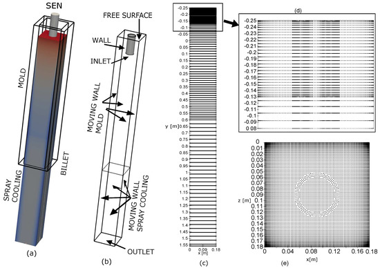
Figure 1. (a) A simplified schematic representation of the continuous casting (CC) of steel. (b) boundary conditions for the simplified CC model; (c) Domain discretization of xy and zy planes for the simplified CC model; (d) close-up of the top of the billet; (e) domain discretization of the yz plane.

2.1.1. Governing Equations

In the present work, we treat incompressible turbulent unsteady fluid flow in a 3D Cartesian coordinate system with position vector $\mathbf{r}=x{\widehat{\mathbf{e}}}_x+y{\widehat{\mathbf{e}}}_y+z{\widehat{\mathbf{e}}}_z$, where x, y, z are coordinates and ${\widehat{\mathbf{e}}}_{\zeta }$, $\zeta =x,y,z$, are standard basis vectors. For the densities ($\rho ={\rho }_L={\rho }_S$), a constant and equal value for both phases ℘ ($\wp =S$ for the solid and $\wp =L$ for the liquid phase) is assumed in the present simplified model. The macroscopic mass conservation equation in the assumed system is

$$\nabla ·\mathbf{u}=0,\mathbf{u}=f_L{\mathbf{u}}_L+f_S{\mathbf{u}}_S,$$

(1)

where mixture velocity $\mathbf{u}$ is a linear combination of the phase velocities ${\mathbf{u}}_{\wp }$ and the phase volume fractions $f_{\wp }$ ($f_S+f_L=1$). The macroscopic momentum equation is

$$\rho \frac{\partial \mathbf{u}}{\partial t}+\rho \nabla ·\left(\mathbf{u}\mathbf{u}\right)=-\nabla p+\nabla ·\left[({\mu }_L+{\mu }_{t,model})(\nabla \mathbf{u}+{(\nabla \mathbf{u})}^T)\right]-\frac{2}{3}\rho \nabla k-{\mu }_L\frac{{(1-f_L)}^2}{C{f}_L^3}(\mathbf{u}-{\mathbf{u}}_S)+\rho {\beta }_T\mathbf{g}(T-T_{ref}),$$

(2)

where t is time, p is pressure, ${\mu }_L$ is the dynamic viscosity, ${\mu }_{t,model}$ is the turbulent dynamic viscosity ($model=RANS$ for RANS turbulent model and $model=LES$ for LES turbulent models), k is the turbulent kinetic energy, C is the morphology constant in porous media, which is considered constant and set to $1.6\times {10}^{-8}$ m${}^2$, ${\beta }_T$ is the thermal expansion coefficient, $\mathbf{g}$ is the constant gravitational acceleration of 9.81 m/s${}^2$, T is the temperature, and $T_{ref}$ is the reference temperature. Flow through porous media is described by the Darcy source term (Term 6) and the Kozeny–Carman relation [31,32], and buoyancy is described by the Boussinesq approximation (Term 7). The macroscopic energy equation is written in the enthalpy formulation as

$$\rho \frac{\partial h}{\partial t}+\rho \nabla ·\left(\mathbf{u}h\right)=\nabla ·(\lambda \nabla T)+\rho \nabla ·(\mathbf{u}h-f_S{\mathbf{u}}_S{h}_S-f_L{\mathbf{u}}_L{h}_L)+\nabla ·\left(f_L\frac{{\rho }_L{\mu }_{t,model}}{\rho {\sigma }_{t,model}}\nabla h_L\right),$$

(3)

where the mixture enthalpy $h=f_L{h}_L+h_S{f}_S$ is a linear combination of phase volume fractions $f_{\wp }$ and phase enthalpies $h_{\wp }$ expressed by temperature-enthalpy relations as

$$h_S={\int }_{T_{ref}}^T{c}_{pS}dT,$$

(4)

for the solid phase, and as

$$h_L={\int }_{T_{ref}}^{T_S}{c}_{pS}dT+{\int }_{T_S}^T{c}_{pL}dT+h_m,$$

(5)

for the liquid phase. The $c_{p\wp }$ is temperature-dependent phase-specific heat at constant pressure and $h_m$ is the melting enthalpy. The $\lambda$ describes the thermal conductivity, and ${\sigma }_{t,model}$ represents the turbulent Prandtl number, which is constant and set to ${\sigma }_{t,RANS}=0.9$ for RANS and to ${\sigma }_{t,LES}=0.4$ for LES turbulence models.

The temperature and the fluid fraction are coupled by the microsegregation model according to Lever’s rule

$$f_L=1-\frac{1}{1-k_p}\frac{T-T_L}{T-T_m},$$

(6)

where $k_p$ is the partition coefficient and $T_m$ is the melting temperature.

2.1.2. Turbulence Modeling

In the LES model, the sub-grid scale or turbulent viscosity is modelled with the Smagorinsky–Lilly [24,25] model as

$${\mu }_{t,LES}=\rho L_S^2\sqrt{2\mathbf{S}:\mathbf{S}},$$

(7)

with the mixing length for sub-grid scales $L_S=min({\kappa }_{vK}\delta ,f_{\mu ,LES}{C}_S\Delta )$, where ${\kappa }_{vK}=0.42$ is von Karman constant, $\delta$ is the normal distance to the nearest walls, $f_{\mu ,LES}=1-exp(y_{LES}^{+}/A^{+})$ is the van Driest damping function with $A^{+}=26$ and

$$y_{LES}^{+}=\frac{\rho \delta u_{\tau }}{\mu },$$

(8)

representing the dimensionless distance to the walls. The damping function is applied to correct the over-dissipation in the Smagorinsky model [33]. $C_S=0.168$ is the Smagorinsky constant, and $\Delta$ is filter width. The normal distance to the nearest wall ($\delta$), which represents the boundary of the solid phase and the outer walls of the billet, is calculated as $\delta =\sqrt{d_x^2+d_y^2+d_z^2}$, where $d_{\zeta }$, $\zeta =x,y,z$ represents the distances in x, y, and z directions. The friction velocity $u_{\tau }=\sqrt{{\tau }_{wall}/\rho }$ is calculated from wall shear stress ${\tau }_{wall}$ and density. The rate of strain tensor is $\mathbf{S}=1/2[\nabla \mathbf{u}+{(\nabla \mathbf{u})}^T]$.

The RANS model, specifically the two-equation Low-Re $k-\epsilon$ model, is used for comparison. In this model, the turbulent kinetic energy is modelled as

$$\rho \frac{\partial k}{\partial t}+\rho \nabla ·\left(\mathbf{u}k\right)=\nabla ·\left[\left({\mu }_L+\frac{{\mu }_{t,RANS}}{{\sigma }_k}\right)\nabla k\right]+P_k+G_k-\rho \epsilon +\rho D-{\mu }_L\frac{{(1-f_L)}^2}{C{f}_L^3}k$$

(9)

and the dissipation rate $\epsilon$ as

$$\rho \frac{\partial \epsilon }{\partial t}+\rho \nabla ·\left(\mathbf{u}\epsilon \right)=\nabla ·\left[\left({\mu }_L+\frac{{\mu }_{t,RANS}}{{\sigma }_{\epsilon }}\right)\nabla \epsilon \right]+[c_{1\epsilon }{f}_1(P_k+c_{3\epsilon }{G}_k)-c_{2\epsilon }{f}_2-\rho \epsilon ]\frac{\epsilon }{k}+\rho E-{\mu }_L\frac{{(1-f_L)}^2}{C{f}_L^3}\epsilon .$$

(10)

The closure coefficients ${\sigma }_k=1.50$, ${\sigma }_{\epsilon }=1.90$, $c_{1\epsilon }=1.40$, $c_{2\epsilon }=1.40$, and $c_{3\epsilon }=tanh|\overline{{\mathbf{u}}_{\parallel }}/\overline{{\mathbf{u}}_{\perp }}|$, damping functions $f_1=1.0$, and

$$f_2={\left(1-{exp}^{-y_{RANS}^{+}/3.1}\right)}^2\left(1-0.3{exp}^{-{(R{e}_t/6.5)}^2}\right),$$

(11)

and source terms in k ($D=0$), and in $\epsilon$ equation ($E=0$) are taken from the AKN model [18]. The $\overline{\mathbf{u}}$ represents the mean value of velocity with ‖ representing parallel and ⊥ perpendicular velocity components. The dimensionless distance to the walls is defined as

$$y_{RANS}^{+}=\frac{{\rho }^{3/4}{\epsilon }^{1/4}\delta }{{\mu }^{3/4}}.$$

(12)

The turbulent Reynolds number is

$$R{e}_t=\frac{\rho k^2}{\mu \epsilon }.$$

(13)

The k production term is written as

$$P_k={\mu }_{t,RANS}\nabla \overline{\mathbf{u}}:[\nabla \overline{\mathbf{u}}+{(\nabla \overline{\mathbf{u}})}^T],$$

(14)

with turbulent dynamic viscosity calculated as

$${\mu }_{t,RANS}=\rho c_{\mu }{f}_{\mu ,RANS}\frac{k^2}{\epsilon },$$

(15)

where closure coefficient $c_{\mu }=0.09$ and damping function

$$f_{\mu ,RANS}={\left(1-{exp}^{-y_{RANS}^{+}/14}\right)}^2\left(1+\frac{5}{R{e}_t^{3/4}}{exp}^{-{(R{e}_t/200)}^2}\right)$$

(16)

are adopted from the AKN model. The generation of turbulence due to the buoyancy force is

$$G_k=-\mathbf{g}{\beta }_T\frac{{\mu }_{t,RANS}}{\rho {\sigma }_{t,RANS}}\frac{\partial T}{\partial y}.$$

(17)

2.1.3. Boundary Conditions

The boundary conditions are required for inlet, meniscus, submerged entry nozzle (SEN) wall, moving walls, and outlet (see Figure 1b). First, the general boundary conditions, which are the same for both turbulence models, are listed. These boundary conditions include restrictions for pressure, temperature, and velocity. Next, the additional values required for each of the models are presented. The LES model requires the turbulent velocity condition at the inlet, whereas the RANS model requires additional restrictions for k and $\epsilon$. The general boundary conditions are:

• Inlet: $u_x=0$ m/s, $u_y=u_{in}$, $u_z=0$ m/s, $T=T_{cast}$, $\partial p/\partial \mathbf{n}=0$ Pa/m;
• Meniscus: $\partial u_x/\partial \mathbf{n}=0$ s${}^{-1}$, $u_y=0$ m/s, $\partial u_z/\partial \mathbf{n}=0$ s${}^{-1}$, $\partial T/\partial \mathbf{n}=0$ K/m, $\partial p/\partial \mathbf{n}=0$ Pa/m;
• SEN wall: $\left|\mathbf{u}\right|=0$ m/s, $T=T_{cast}$, $\partial p/\partial \mathbf{n}=0$ Pa/m;
• Moving walls: $u_x=0$ m/s, $u_y=u_{cast}$, $u_z=0$ m/s, $q_{cz}=h_{cz}(T-T_0)$, where $q_{cz}$ is heat flux and $h_{cz}=h_{mo}$ in the mold and $h_{cz}=h_{sc}$ in the secondary cooling zone, $\partial p/\partial \mathbf{n}=0$ Pa/m;
• Outlet: $\partial \mathbf{u}/\partial \mathbf{n}=0$ s${}^{-1}$, $\partial T/\partial \mathbf{n}=0$ K/m, $p=0$ Pa.

The additional boundary conditions for the LES model are applied only at the inlet and are:

• Inlet: The synthetic turbulence approach proposed by [27,29] is used to generate the velocity fluctuations. The method proposes the decomposition of velocity into Fourier series

  $$\mathbf{u}\left(\mathbf{r}\right)=2\sum _{m=1}^M{q}_{m}cos({\kappa }_m{\widehat{\mathbf{k}}}_m·\mathbf{r}+{\psi }_m){\widehat{\sigma }}_m,$$

  (18)

  where M is the number of modes, $q=\sqrt{E\left(\kappa \right)\Delta \kappa }$ is the wave amplitude of the mode, with the turbulent kinetic energy of LES model $E\left(\kappa \right)$ described by the modified von Karman–Pao spectrum as

  $$E\left(\kappa \right)=\alpha \frac{u_{rms}^2}{{\kappa }_e}\frac{{(\kappa /{\kappa }_e)}^4}{{[1+{(\kappa /{\kappa }_e)}^2]}^{17/6}}{exp}^{-2{(\kappa /{\kappa }_{\eta })}^2}.$$

  (19)
  The $\kappa$ is wave number, $\widehat{k}$ is a unit direction vector of the wave number, $\sigma$ is phase angle, and $\widehat{\sigma }$ is a unit direction, $\alpha =1.453$ is a scaling constant, ${\kappa }_e=40\sqrt{5/12}$ is a wave number of maximum energy, ${\kappa }_{\eta }={\epsilon }_{LES}^{1/4}{\mu }^{-3/4}rh{o}^{3/4}$ is the Kolmogorov wave number, ${\epsilon }_{LES}=u_{rms}^3/L$, $u_{rms}={(2/3k_0)}^{1/2}$ is the root mean square of velocity fluctuations, $L=0.746834{\kappa }_e$ is integral length scale. The condition ${\widehat{\mathbf{k}}}_m·{\widehat{\sigma }}_m=0$ must be fulfilled at all times. Additionally, the time correlation is established by applying the asymmetric time correlation filter as

  $${\mathbf{u}}^{n+1}=a{\mathbf{u}}^n+b{\mathbf{u}}_{inlet},$$

  (20)

  where $a=exp(-\Delta t/\tau )$ with $\tau =0.05/u_{in}$, $b=\sqrt{1-a^2}$, and inlet velocity defined as ${\mathbf{u}}_{inlet}=f_{blend}\mathbf{u}\left(\mathbf{r}\right)$ with blending function $f_{blend}=max[0.5(1-tanh(\{\delta -{\delta }_{bl}\}/{\delta }_{ew})),0.1]$ with boundary layer thickness ${\delta }_{bl}=0.1$ and effective width of the blending function ${\delta }_{ew}=0.5$.

The additional boundary conditions for the RANS model are:

• Inlet: $k_0=3/2{\left(I{u}_{in}\right)}^2$, where $I=0.16R{e}^{-1/8}$ represents semi-empirical correlation for the turbulent intensity in pipe flows, ${\epsilon }_0=C_{\mu }^{3/4}{k}_0^{3/2}/\left(0.07L_c\right)$, where $L_c$ is characteristic length;
• Meniscus: $\partial k/\partial \mathbf{n}=0$ m/s${}^2$, $\partial \epsilon /\partial \mathbf{n}=0$ m/s${}^3$;
• SEN wall: $\partial k/\partial \mathbf{n}=0$ m/s${}^2$, $\partial \epsilon /\partial \mathbf{n}=0$ m/s${}^3$;
• Moving walls: $\partial k/\partial \mathbf{n}=0$ m/s${}^2$, $\partial \epsilon /\partial \mathbf{n}=0$ m/s${}^3$;
• Outlet: $\partial k/\partial \mathbf{n}=0$ m/s${}^2$, $\partial \epsilon /\partial \mathbf{n}=0$ m/s${}^3$.

The values for process parameters are listed in Table 1.

Table 1. Process parameters and billet domain dimensions.

Parameter	Notation	Value
Casting velocity	$u_{cast}$	0.027 m/s
Inlet velocity	$u_{in}$	$4u_{cast}{l}_3^2/\left(\pi l_1^2\right)$
Ambient temperature	$T_0$	293.15 K
Heat transfer coefficient in the mold	$h_{mo}$	2000 W/(m${}^2$ K)
Heat transfer coefficient in the secondary cooling zone	$h_{sc}$	800 W/(m${}^2$ K)
Casting temperature	$T_{cast}$	1798 K
Submerged entry nozzle (SEN) inner width	$l_1$	0.035 m
SEN outer width	$l_{1out}$	0.065 m
SEN immersion depth	$l_2$	0.15 m
Mold width	$l_3$	0.18 m
Mold height	$l_4$	0.85 m
Billet length	$l_5$	1.8 m

2.2. Numerical Method and Solution Procedure

2.2.1. Discretization

The discretization of the 3D computational domain is constructed from horizontal slices (see Figure 1e) stacked in the vertical direction (see Figure 1c). The refinement is calculated as

$${\zeta }_i^{refined}={\zeta }_{max}-({\zeta }_{max}-{\zeta }_{min}){\left(1.0-\frac{(i-1)}{N_i-1}\right)}^{bi},$$

(21)

where $\zeta =x,y,z$, ${\zeta }_i^{refined}$ represents the position of the i-th node, ${\zeta }_{max}$ is the maximum height of the refinement interval, ${\zeta }_{min}$ is the minimum height of the refinement interval, $i=1,2,\cdots ,N_i$, $N_i$ is the number of nodes in the refinement interval, and $bi$ is the refinement parameter. The schematic representation of the refinement process is depicted in Figure 2. The refinement in the vertical (y) direction is constructed from three parts: the SEN, the mold, and the secondary cooling region. The maximum refinement is implemented in the SEN region (see Figure 1d), where the largest gradients of the flow field are expected. The refinement parameter in the SEN region is set to $bi=2.0$ in both directions, in mold to $bi=1.8$ in both directions, and in the secondary cooling region to $bi=1.6$ towards the top of the region. The total number of vertically stacked slices is 45. The refinement in the horizontal slices (see Figure 1e) is applied towards the wall, where $bi=2.0$. The schematic representation of the refinement process is depicted in Figure 2. The total number of nodes used in the calculation is 1,044,344, which is the largest model computed with this method up to date. The discretization is coded in Fortran 95 programming language and is part of the pre-processing portion of the solution procedure.

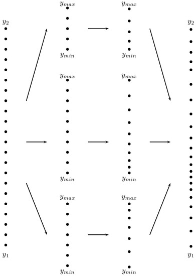
Figure 2. The schematic representation of the refinement process.

2.2.2. Local Radial Basis Function Collocation Method

The Euler explicit method is used for time discretization along with Courant–Friedrichs–Levy $\lambda \Delta t/{\zeta }_{max}^2<1/2$ and von Neumann $\left|\mathbf{u}\right|\Delta t/{\zeta }_{max}<1$ stability criteria. The ${\zeta }_{max}$ represents the maximum distance between nodes in each direction. The strong-form meshless local collocation method is used for space discretization. The method employs scaled multiquadric (MQ) RBF

$$\psi =\sqrt{{\left(\frac{x-x_l}{x_{lmax}}\right)}^2+{\left(\frac{y-y_l}{y_{lmax}}\right)}^2+{\left(\frac{z-z_l}{z_{lmax}}\right)}^2+c^2},$$

(22)

as shape functions with shape parameter $c=32$ and scaling parameter ${\zeta }_{lmax}$, $\zeta =x,y,z$ in sub-domain l. In 3D, seven nodded sub-domains are used. A schematic representation of the MQ RBF is presented in Figure 3.

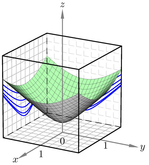
Figure 3. The schematic representation of multiquadric (MQ) radial basis functions (RBF) with shape parameter $c=0.25$.

Although we have previously successfully implemented the 2D LES model with LRBFCM discretization in the CC of steel, we now present the extension of this model to 3D. The filter width is in 3D defined as $\Delta =V^{1/3}$, with $V=d_{x/2}{d}_{y/2}{d}_{z/2}$, where $d_{\zeta /2}=d_{\zeta max}/2$ ($\zeta =x,y,z$) represents half of the maximum distance $d_{\zeta max}$ between nodes in the sub-domain.

2.2.3. Solution Procedure

The solution procedure begins with the pre-processing part (see Figure 4a), where we set the node arrangement, construct sub-domains, calculate constant variables, initial and boundary conditions. The main loop, schematically depicted in the block diagram in Figure 4b, closely follows the solution procedure described in [3]. The new addition to the solution procedure described in [3] is the switch between different turbulence models and the 3D application of LES. The pressure–velocity coupling is solved by the fractional step method (FSM) [34], and the highly convective flow is stabilized by an upwinding scheme described in [3].

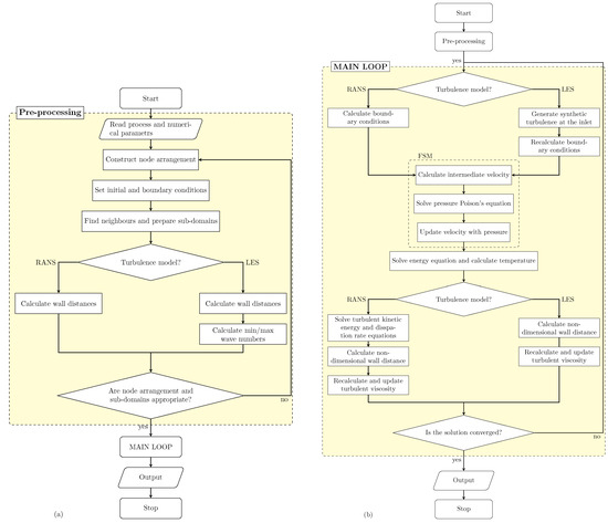
Figure 4. The schematic representation of the solution procedure. (a) scheme of the pre-processing block diagram; (b) scheme of the main loop block diagram.

The solution procedure of 3D isotropic turbulence at the inlet closely follows the procedure described in [27,28,29]. The procedure begins by constructing the minimum ${\kappa }_{min}=min\left(2\pi d_{\zeta max}\right)$ and maximum ${\kappa }_{max}=max(\pi /d_{\zeta min})$ wave numbers, where $d_{\zeta min}$ stands for minimum none-zero distances in the $\zeta =x,y,z$ direction between nodes in the local sub-domain. Next, we divide the wave spectrum into $M=150$ modes to obtain ${\kappa }_m={\kappa }_{min}+({\kappa }_{max}-{\kappa }_{min})(m-1)/M$; ($m=1,\cdots ,M$). We then chose the random functions ${\alpha }_m$, ${\psi }_m$, ${\theta }_m$, and ${\varphi }_m$. The probability distributions for random functions are given in Table 2. Following is the computation of the wave vectors:

$$k_{x,m}=sin\left({\theta }_m\right)cos\left({\varphi }_m\right),$$

(23)

$$k_{y,m}=sin\left({\theta }_m\right)sin\left({\varphi }_m\right),$$

(24)

$$k_{y,m}=cos\left({\theta }_m\right).$$

(25)

Table 2. Probability distribution of random functions [27].

Probability Distribution	Probability Interval
$p\left({\alpha }_m\right)=1/\left(2\pi \right)$	$0\le {\alpha }_m\le 2\pi$
$p\left({\varphi }_m\right)=1/\left(2\pi \right)$	$0\le {\varphi }_m\le 2\pi$
$p\left({\psi }_m\right)=1/\left(2\pi \right)$	$0\le {\psi }_m\le 2\pi$
$p\left({\theta }_m\right)=sin\left(\theta \right)/2$	$0\le {\theta }_m\le \pi$

The unit vector is then calculated as

$${\sigma }_{x,m}=cos\left({\theta }_m\right)cos\left({\varphi }_m\right)cos\left({\alpha }_m\right)-sin\left({\varphi }_m\right)sin\left({\alpha }_m\right),$$

(26)

$${\sigma }_{y,m}=cos\left({\theta }_m\right)sin\left({\varphi }_m\right)cos\left({\alpha }_m\right)-cos\left({\varphi }_m\right)sin\left({\alpha }_m\right),$$

(27)

$${\sigma }_{y,m}=-sin\left({\theta }_m\right)cos\left({\alpha }_m\right).$$

(28)

For every mode M, we then calculate $q_m=\sqrt{E\left({\kappa }_m\right)\Delta \kappa }$. Finally, we can calculate the velocity (Equation (18)) at each node in the computational domain.

2.2.4. Numerical Implementation

The numerical solution is coded in Fortran 95 programming language. The results were calculated on an Intel i7-9850H processor that runs on 12 cores at 2.60 GHz and a 64 bit Windows 10 operating system. The calculation time for $k-\epsilon$ model is approximately 21 days to reach the steady state. The LES model calculation lasted approximately 60 days to obtain a reasonably good statistical time average.

3. Results

3.1. Geometry and Process Parameters

The geometry and the computational domain of the continuous casting process are depicted in Figure 1. The computational domain is constructed from a square billet with centrally placed SEN with width $l_1$ and immersion depth $l_2$. The billet height $l_5$ is split into mold region $l_4$ and spray cooling region $l_5-l_4$. The dimensions of the billet are listed in Table 1 along with process parameters.

3.2. Material Properties

Although the material properties of steel are temperature dependent, a simplified, constant and equal values are used for both phases in the present paper. The exceptions are the values for specific heat. The material properties are presented in Table 3.

Table 3. Material properties of steel.

Property	Notation	Value
Thermal conductivity	$\lambda$	33 W/(mK)
Density	$\rho$	7300 kg/m${}^3$
Specific heat in solid	$c_{pS}$	698 J/(kg K)
Specific heat in liquid	$c_{pL}$	804 J/(kg K)
Solidus temperature	$T_S$	1673 K
Liquidus temperature	$T_L$	1755 K
Mold enthalpy	$h_m$	173,404 J/kg
Melting temperature	$T_m$	1812 K
Dynamic viscosity	$\mu$	$6\times {10}^{-3}$ Pa s
Thermal expansion coefficient	${\beta }_T$	$1\times {10}^{-4}$ 1/K

3.3. Numerical Results and Discussion

The numerical solutions for LES and RANS have been previously thoroughly tested on benchmark results [35,36,37]. The results are compared for horizontal (HA1 ($xz$ plane): $y=0.19$ m) and vertical (VA1 ($zy$ plane): $x=0.18$ m, VA2 ($xy$ plane): $z=0.09$ m, VA3 (y plane: $x=z$) planes as well as horizontal (HL1 ($xz$ plane): $y=0.19$ m, $z=0.09$ m; HL2 ($xz$ plane, $y=0.19$ m, $x=z$) and vertical (VL1 ($xy$ plane): $x=0.09$ m, $z=0.09$ m; VL2 ($xy$ plane): $x=0.18$ m, $z=0.09$ m) cross-sections as depicted in Figure 5. The time average for LES model is calculated over a time period of 1400 s.

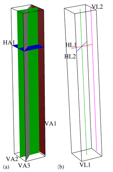
Figure 5. Schematic representation of cross-section planes and lines. (a) cross-section planes: blue—HA1 ($xz$ plane: $y=0.19$ m), red—VA1 ($zy$ plane: $x=0.18$ m), gray—VA3 (y plane: $x=z$), green—VA2 ($xy$ plane: $z=0.09$ m). (b) Cross-section lines: red—HL1 ($xz$ plane, $y=0.19$ m, $z=0.09$ m), blue—HL2 $xz$ plane, $y=0.19$ m, $x=z$, green—VL1 ($xy$ plane, $x=0.09$ m, $z=0.09$ m), magenta—VL1 ($xy$ plane, $x=0.18$ m, $z=0.09$ m).

Temperature fields were examined first for HA1 cross-section and are shown in Figure 6 for $k-\epsilon$ and LES models. The temperatures in the central area are lower for $k-\epsilon$ model, where the highest temperature in HA1 cross-section reaches 1517.60 ${}^{\circ }$C and the lowest is 551.92 ${}^{\circ }$C. The highest and lowest temperatures in the LES model for HA1 are 1524.96 ${}^{\circ }$C and 553.54 ${}^{\circ }$C in Figure 6b, 1524.98 ${}^{\circ }$C and 552.26 ${}^{\circ }$C in Figure 6c, and 1524.95 ${}^{\circ }$C and 557.74 ${}^{\circ }$C in Figure 6d. The difference in the highest and in the lowest temperature between both models is around 5 ${}^{\circ }$C. In the LES model, the cooling in the central area is slower due to the oscillations that can also be seen in the shape of the higher temperature area in the center of the billet.

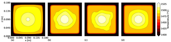
Figure 6. Temperature field at HA1. (a) $k-\epsilon$ model; steady-state; (b) Large-eddy simulation (LES) model at $t_1=205$ s; (c) LES model at $t_2=1096$ s; (d) LES model; time-average.

Figure 7 shows the temperature field area cross-section at VA2. The steady-state solution of the $k-\epsilon$ model results in lower temperatures in the center of the billet and around SEN. The maximum difference in the temperatures between both models is approximately 30 ${}^{\circ }$C as shown in Figure 8.

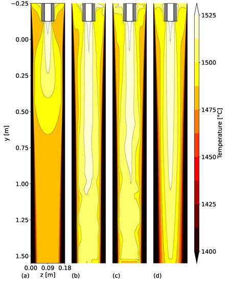
Figure 7. Temperature field at VA2. (a) $k-\epsilon$ model; steady-state; (b) LES model at $t_1=205$ s; (c) LES model at $t_2=1096$ s; (d) LES model; time-average.

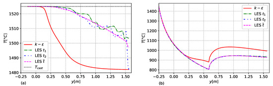
Figure 8. Temperature field. (a) At VL1; (b) At VL2.

Figure 9 shows the temperature field area cross-section at VA3. As in the VA2 cross-section, the steady-state solution of the $k-\epsilon$ model results in lower temperatures in the center of the billet and around the SEN.

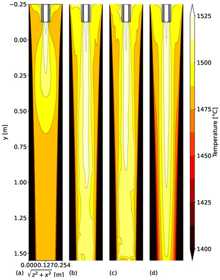
Figure 9. Temperature field at VA3. (a) $k-\epsilon$ model; steady-state; (b) LES model at $t_1=205$ s; (c) LES model at $t_2=1096$ s; (d) LES model; time-average.

The temperature profile at the wall of the billet is presented in Figure 10. The temperatures at the mold-secondary cooling zone transition are lower in the LES model, similar to the case of EMS [3].

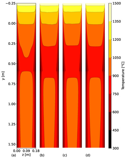
Figure 10. Temperature field at VA1. (a) $k-\epsilon$ model; steady-state; (b) LES model at $t_1=205$ s; (c) LES model at $t_2=1096$ s; (d) LES model; time-average.

Figure 8 shows the vertical line cross-section at VL1 and VL2 (see Figure 5b). In the LES model, the temperature is higher at the center (see Figure 11a) and lower at the wall (see Figure 11b). The influence of the LES turbulence model at the wall is similar to the influence of EMS [3].

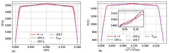
Figure 11. Temperature field. (a) At HL1; (b) At HL2.

Figure 11 shows the horizontal line cross-section at HL1 and HL2 (see Figure 5b). For both cross-sections, the temperatures at height $y=0.19$ m for both models are very similar and differ at a maximum for only 5 ${}^{\circ }$C.

Velocity magnitude field at HA1 is depicted in Figure 12 for $k-\epsilon$ and LES models. The velocity in the LES model is higher in the center of the billet and as expected fluctuates. In the $k-\epsilon$ model, there are four recirculation zones—one in each corner that do not appear in the time-averaged results of the LES model. Consequently, the velocity magnitude in this region is higher in the $k-\epsilon$ model. The highest velocity magnitude in the $k-\epsilon$ model in the HA1 cross-section area is 0.691 m/s, and the lowest is 0.0091 m/s. The highest and lowest velocity magnitudes in the LES model for HA1 in the examples shown are 0.8925 m/s and 0.004926 m/s in Figure 12b, 0.8943 m/s and 0.0009220 m/s in Figure 12c, and the time average of velocity magnitude in plane HA1 is 0.8838 m/s and 0.0003 m/s (Figure 12d).

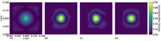
Figure 12. Velocity magnitude field at HA1. (a) $k-\epsilon$ model; steady-state; (b) LES model at $t_1=205$ s; (c) LES model at $t_2=1096$ s; (d) LES model; time-average.

The velocity vectors are plotted in Figure 13. The $k-\epsilon$ model shows that the velocity in the mold circulates in the vertical direction. In the LES model, the circulation is also in a horizontal direction as shown in Figure 13b–d and is similar to [3].

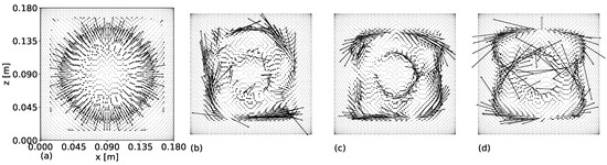
Figure 13. Velocity vectors at HA1. (a) $k-\epsilon$ model; steady-state; (b) LES model at $t_1=205$ s; (c) LES model at $t_2=1096$ s; (d) LES model; time-average.

Figure 14 and Figure 15 show the vertical velocity magnitude cross-sections (VA3 and VA2—see Figure 5). The steady-state solution of $k-\epsilon$ model shows that the higher velocity range is much shorter than in the LES models. The recirculation zones can be seen in the diagonal cross-section VA3 in Figure 14.

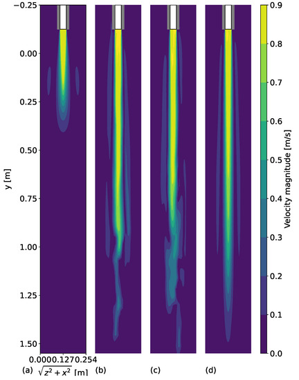
Figure 14. Velocity magnitude field at VA3. (a) $k-\epsilon$ model; steady-state; (b) LES model at $t_1=205$ s; (c) LES model at $t_2=1096$ s; (d) LES model; time-average.

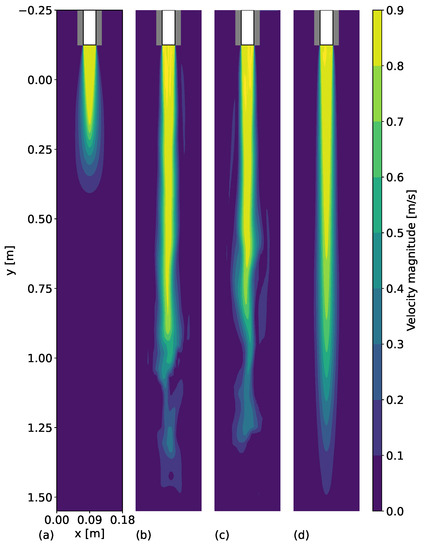
Figure 15. Velocity magnitude field at VA2. (a) $k-\epsilon$ model; steady-state; (b) LES model at $t_1=205$ s; (c) LES model at $t_2=1096$ s; (d) LES model; time-average.

Figure 16 shows the vertical line cross-section of velocity magnitude for both turbulence models. The oscillations of velocity at the inlet in the LES turbulence model are due to the applied synthetic turbulence at the inlet. The central velocity of $k-\epsilon$ model falls to casting velocity at approximately 0.5 m, whereas, in the LES model, the central velocity is higher and approaches casting velocity at about 1.5 m. This is due to the transient nature of the model. It should also be noted that, below the mold, the oscillations become bigger.

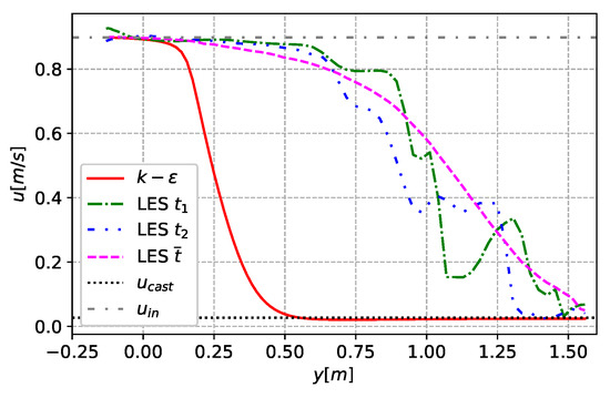
Figure 16. Velocity field at VL1.

Figure 17 shows a horizontal line cross-section at HL1 and HL2 (see Figure 5b). The velocity at height $y=0.19$ m is smaller for the $k-\epsilon$ model and has narrower distribution. The oscillations of velocity are larger in diagonal cross-section for both examples as shown in Figure 17b.

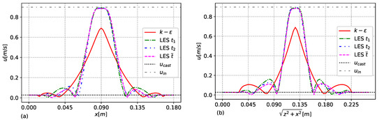
Figure 17. Velocity field. (a) at HL1; (b) at HL2.

4. Conclusions

The solution of the LES turbulence model by an LRBFCM is demonstrated for the first time for a 3D CC process and is compared to the previous results calculated with a RANS turbulence model [3]. The solution procedure is divided into two parts. The first part is the preprocessing part, where constants such as wall distances and minimum and maximum wavenumbers are specified for each of the applied turbulence models. The second part describes the main part of the solution procedure, where the governing equations and constitutive relations are solved. The simplified application of geometry, boundary conditions, and material properties is used to facilitate a comparison of the current model with previous applications. The simulated problem has 1,044,344 nodes, the most enormous problem calculated to date using the LRBFCM.

The results are compared to the steady-state solution of the $k-\epsilon$ turbulence model. The LES solution leads to higher central temperatures and velocities. The temperature line cross-section of the LES model is similar to the results of the EMS model. The LES model also shows recirculation of flow in the horizontal direction, similar to the effects of EMS. The results obtained with the LES model are more detailed. However, they require a larger number of nodes at a considerably higher computational time.

The ability of the method shown in this work to solve complicated transient swirling flow problems will allow for tackling a large spectrum of realistic industrial problems in the future.

References

- Šarler, B.; Vertnik, R.; Mramor, K. A numerical benchmark test for continuous casting of steel. IOP Conf. Ser. Mater. Sci. Eng. 2012, 33, 012012. [Google Scholar] [CrossRef]
- Mramor, K.; Vertnik, R.; Šarler, B. Simulation of continuous casting of steel under the influence of magnetic field using the local-radial basis-function collocation method. Mater. Tehnol. 2014, 48, 281–288. [Google Scholar]
- Vertnik, R.; Mramor, K.; Šarler, B. Solution of three-dimensional temperature and turbulent velocity field in continuously cast steel billets with electromagnetic stirring by a meshless method. Eng. Anal. Bound. Elem. 2019, 104, 347–363. [Google Scholar] [CrossRef]
- Mramor, K.; Vertnik, R.; Šarler, B. Meshless approach to the large-eddy simulation of the continuous casting process. Eng. Anal. Bound. Elem. 2022, 138, 319–338. [Google Scholar] [CrossRef]
- Chaudhary, R.; Ji, C.; Thomas, B.G.; Vanka, S.P. Transient turbulent flow in a liquid-metal model of continuous casting, including comparison of six different methods. Metall. Mater. Trans. B Process Metall. Mater. Process. Sci. 2011, 42, 987–1007. [Google Scholar] [CrossRef]
- Javurek, M.; Barna, M.; Gittler, P.; Rockenschaub, K.; Lechner, M. Flow Modelling in Continuous Casting of Round Bloom Strands with Electromagnetic Stirring. Steel Res. Int. 2008, 79, 617–626. [Google Scholar] [CrossRef]
- Liu, Z.Q.; Qi, F.S.; Li, B.K.; Fumitaka, T. Large eddy simulation for unsteady turbulent field in thin slab continuous casting mold. J. Iron Steel Res. Int. 2012, 18, 243–250. [Google Scholar] [CrossRef]
- Liu, Z.; Li, B. Transient motion of inclusion cluster in vertical-bending continuous casting caster considering heat transfer and solidification. Powder Technol. 2016, 287, 315–329. [Google Scholar] [CrossRef]
- Singh, R.; Thomas, B.G.; Vanka, S.P. Large eddy simulations of double-ruler electromagnetic field effect on transient flow during continuous casting. Metall. Mater. Trans. B Process Metall. Mater. Process. Sci. 2014, 45, 1098–1115. [Google Scholar] [CrossRef]
- Jin, K.; Vanka, S.P.; Thomas, B.G. Large eddy simulations of electromagnetic braking effects on argon bubble transport and capture in a steel continuous casting mold. Metall. Mater. Trans. B Process Metall. Mater. Process. Sci. 2018, 49, 1360–1377. [Google Scholar] [CrossRef]
- Ji, C.B.; Li, J.S.; Yang, S.F.; Sun, L.Y. Large Eddy Simulation of Turbulent Fluid Flow in Liquid Metal of Continuous Casting. J. Iron Steel Res. Int. 2013, 20, 34–39. [Google Scholar] [CrossRef]
- Li, X.; Li, B.; Liu, Z.; Niu, R.; Liu, Y.; Zhao, C.; Huang, C.; Qiao, H.; Yuan, T. Large eddy simulation of multi-phase flow and slag entrapment in a continuous casting mold. Metals 2019, 9, 7. [Google Scholar] [CrossRef]
- Chen, W.; Ren, Y.; Zhang, L. Large Eddy Simulation on the Fluid Flow, Solidification and Entrapment of Inclusions in the Steel Along the Full Continuous Casting Slab Strand. Jom 2018, 70, 2968–2979. [Google Scholar] [CrossRef]
- Vakhrushev, A.; Liu, Z.; Wu, M.; Kharicha, A.; Ludwig, A.; Nitzl, G.; Tang, Y.; Hackl, G. Numerical modelling of the MHD flow in continuous casting mold by two CFD platforms ANSYS Fluent and OpenFOAM. In Proceedings of the ICS 2018—7th International Congress on Science and Technology of Steelmaking: The Challenge of Industry 4.0, Venice, Italy, 3–15 June 2018. [Google Scholar]
- Sivaramakrishnan, S. Large Eddy Simulation, Particle Image Velocimetry in the Study of Mold Transients in Continuous Casting of Steel and Heat Transfer through Molten Slag Layers. Ph.D. Thesis, University of Illinois, Champaign, IL, USA, 2000. [Google Scholar]
- Gregorc, J.; Kunavar, A.; Šarler, B. RANS versus Scale Resolved Approach for Modeling Turbulent Flow in Continuous Casting of Steel. Metals 2021, 11, 1140. [Google Scholar] [CrossRef]
- Yusof, S.N.A.; Asako, Y.; Sidik, N.A.C.; Mohamed, S.B.; Japar, W.M.A.A. A short review on RANS turbulence models. CFD Lett. 2020, 12, 83–96. [Google Scholar] [CrossRef]
- Abe, K.; Kondoh, T.; Nagano, Y. A new turbulence model for predicting fluid flow and heat transfer in separating and reattaching flows-II. Thermal field calculations. Int. J. Heat Mass Transf. 1995, 38, 1467–1481. [Google Scholar] [CrossRef]
- Launder, B. Application of the energy-dissipation model of turbulence to the calculation of flow near a spinning disc. Int. Commun. Heat Mass Transf. 1974, 1, 131–137. [Google Scholar] [CrossRef]
- Vertnik, R. Heat and Fluid Flow Simulation of the Continuous Casting of Steel by a Meshless Method. Ph.D. Thesis, University of Nova Gorica, Nova Gorica, Slovenia, 2010. [Google Scholar]
- Germano, M.; Piomelli, U.; Moin, P.; Cabot, W.H. A dynamic subgrid-scale eddy viscosity model. Phys. Fluids A 1991, 3, 1760–1765. [Google Scholar] [CrossRef]
- Lilly, D.K. A proposed modification of the Germano subgrid-scale closure method. Phys. Fluids A 1992, 4, 633–635. [Google Scholar] [CrossRef]
- Nicoud, F.; Ducros, F. Subgrid-scale stress modelling based on the square of the velocity. Agric. Econ. Res. Rev. 2006, 19, 37–48. [Google Scholar] [CrossRef]
- Smagorinsky, J. General circulation experiments with the primitive equations. Mon. Weather. Rev. 1963, 91, 99–164. [Google Scholar] [CrossRef]
- Lilly, D.K. On the Application of the Eddy Viscosity Concept in the Inertial Sub-Range of Turbulence by; National Center for Atmospheric Research: Boulder, CO, USA, 1966; Volume 123. [Google Scholar]
- Mramor, K.; Vertnik, R.; Šarler, B. Large-eddy simulation of continuous casting process. In Proceedings of the STEEL SIM 2021: 9th International Conference on Modeling and Simulation of Metallurgical Processes in Steelmakin; Wu, M., Ed.; ASMET, Austrian Society for Metallurgy and Materials: Leoben, Austria, 2021; pp. 310–317. [Google Scholar]
- Davidson, L. Using isotropic synthetic fluctuations as inlet boundary conditions for unsteady simulations. Adv. Appl. Fluid Mech. 2007, 1, 1–35. [Google Scholar]
- Davidson, L.; Billson, M. Hybrid LES-RANS using synthesized turbulence for forcing at the interface. In Proceedings of the ECCOMAS 2004—European Congress on Computational Methods in Applied Sciences and Engineering, Jyväskylä, Finland, 24–28 July 2004; pp. 1–18. [Google Scholar]
- Saad, T.; Cline, D.; Stoll, R.; Sutherland, J.C. Scalable tools for generating synthetic isotropic turbulence with arbitrary spectra. AIAA J. 2017, 55, 327–331. [Google Scholar] [CrossRef]
- Baba-Ahmadi, M.H.; Tabor, G. Inlet conditions for LES using mapping and feedback control. Comput. Fluids 2009, 38, 1299–1311. [Google Scholar] [CrossRef]
- Kozeny, J. Ober kapillare Leitung des Wassers im Boden. Akad. Wiss. Wien 1927, 136, 271–306. [Google Scholar]
- Carman, P.G. Fluid flow through granular beds. Chem. Eng. Res. Des. 1997, 75, S32–S48. [Google Scholar] [CrossRef]
- Pakzad, A. Damping functions correct over-dissipation of the Smagorinsky model. Math. Methods Appl. Sci. 2017, 40, 5933–5945. [Google Scholar] [CrossRef]
- Chorin, A.J. On the Convergence of Discrete Approximations to the Navier–Stokes Equations. Math. Comput. 1969, 23, 341. [Google Scholar] [CrossRef]
- Mramor, K.; Vertnik, R.; Šarler, B. Simulation of laminar backward facing step flow under magnetic field with explicit local radial basis function collocation method. Eng. Anal. Bound. Elem. 2014, 49, 37–47. [Google Scholar] [CrossRef]
- Mramor, K.; Vertnik, R.; Šarler, B. Application of the local RBF collocation method to natural convection in a 3D cavity influenced by a magnetic field. Eng. Anal. Bound. Elem. 2020, 116, 1–13. [Google Scholar] [CrossRef]
- Mramor, K.; Vertnik, R.; Šarler, B. Low and intermediate re solution of lid driven cavity problem by Local Radial Basis Function Collocation Method. Comput. Mater. Contin. 2013, 36, 1–21. [Google Scholar] [CrossRef]
Publisher’s Note: MDPI stays neutral with regard to jurisdictional claims in published maps and institutional affiliations. |
© 2022 by the authors. Licensee MDPI, Basel, Switzerland. This article is an open access article distributed under the terms and conditions of the Creative Commons Attribution (CC BY) license (https://creativecommons.org/licenses/by/4.0/).