Article

Processing Tests, Adjusted Cost Models and the Economies of Reprocessing Copper Mine Tailings in Chile

1
Federal Institute for Geosciences and Natural Resources (BGR), Stilleweg 2, 30655 Hannover, Germany
2
G.E.O.S. Ingenieurgesellschaft mbH, Schwarze Kiefern 2, 09633 Halsbruecke, Germany
3
Servicio Nacional de Geología y Minería Av. Santa María, Providencia 0104, Chile
4
German Mineral Resources Agency (DERA) at the Federal Institute for Geosciences and Natural Resources (BGR), Wilhelmstrasse 25-30, 13593 Berlin, Germany
*
Author to whom correspondence should be addressed.
Metals 2021, 11(1), 103; https://doi.org/10.3390/met11010103
Submission received: 4 December 2020 / Revised: 19 December 2020 / Accepted: 20 December 2020 / Published: 6 January 2021

Abstract

:
To increase resource efficiency, mining residues–especially tailings–have come into the focus of research, companies, and politics. Tailings still contain varying amounts of unextracted elements of value and minerals that were not of economic interest during production. As for primary mineral deposits, only a small share of tailings offers the possibility for an economic reprocessing. To minimize exploration expenditure, a stepwise process is followed during exploration, to estimate the likelihood of a project to become a mine or in this case a reprocessing facility. During this process, costs are continuously estimated at least in an order of magnitude. Reprocessing flowsheets for copper mine tailings in Chile were developed and costs and revenues of possible products from reprocessing were examined for a rough economic assessment. Standard cost models with capex and opex for flotation, leaching, and magnetic separation were adopted to the needs of tailings reprocessing. A copper tailing (around 2 M t) that also contains magnetite was chosen as a case study. A combination of magnetic separation and leaching gave the best economic results for copper and magnetite. The adopted cost models showed positive results at this early stage of investigation (semi-technical scale processing tests).

1. Introduction

Copper is by value one of the main mineral commodities in the world [1]. Due to the nature of mineral deposits, not only ore minerals are extracted, but also barren minerals that have to be deposited as tailings [2]. According to [3], more than 500 M t of tailings were produced in Chile, in 2019 alone. Over the past 30 years, more than 7 billion tons of tailings have been stockpiled or discarded in Chile, assuming a copper grade of 2% (most probably lower, leading to even more tailings). In many cases, the tailings still contain some copper and possibly other metals of value with potential for recovery [4,5,6]. The ore processing technology has improved significantly over the last decades, making it possible to mine lower grade ore bodies [7] and reducing the metal grade that enters into a tailings storage facility (TSF) from 0.75% at the beginning of the 20th century to around 0.1% in the late 1990s [8]. This makes old tailings or tailings originating from processing facilities with a non-homogeneous ore feed or with a non-homogeneous copper mineralogy (both factors are harmful for a good recovery) optimal targets for a possible economic reprocessing. Due to weathering, reprocessing is often more cost-intensive compared to primary ore processing, as described by [9] and references therein, for Russia. As tailings have already been floated once, re-flotation in some cases is possible [10], but can result in low recoveries because of non-floatable minerals or very fine grain sizes. The small grain size can at least in part be overcome by using a tailored size distribution of the tailings material [11]. Besides froth flotation, leaching is the second most common method to process copper ore. Leaching can be carried out via conventional sulfuric acid leach or with support of bacteria. An overview of the share of (bio)leaching in copper processing is given by [12]. Bioleaching, especially, is in the focus of research, as it can be an alternative to conventional ore processing, when the share of floatable minerals is too low [12,13,14,15,16,17]. A review about the various possible reuses of mine tailings is given by [18] and references therein. They conclude that: “Various methods have been suggested for recycling but there is a lack of well-documented cost and performance data under a variety of operating conditions.” Nevertheless, a business case is the prerequisite for reprocessing mine waste, unless the environmental harm is so severe that a mining company is forced to intervene or a public agency is funding the cleanup. Different recycling flowsheets need to be designed for every single case study and economic analyses have to be undertaken, to assess the recycling potential. This is especially the case, as the grade of valuable elements in the tailings is not of value, but the recoverable grade–as for any orebody. In the case of tailings, which are influenced by weathering over years or decades, the mineralogy can change due to the climate and make the recovery more challenging [9,19]. Especially a mixture of sulfide and oxide minerals is difficult to process, as a combination of sulfide and oxide flotation or a combination of leaching and flotation have to be applied. Reference [8] showed that there is a substantial amount of copper in tailings, waste rock, and slag, and proposed that this copper would soon be recoverable using new technology. Nevertheless, reprocessing copper tailings remains relatively sparse. Only 30,000 t of copper per year were produced from projects that use tailings as primary source [20]. Assuming that not all tailings reprocessing projects are known and incorporated into the mentioned database, the amount is low compared to the more than 20 M t of copper that is produced by mines every year. Reference [21] describes various possibilities how to reuse mine waste as mineral resource, but also mentions that it is only rarely done due to economic reasons. Actually, it is difficult to give hard facts for capital expenditure (capex) and operating expenditure (opex), when applying new technologies, for which no empirical values or rules of thumb exist. Even for established techniques like flotation or leaching, it is difficult to give cost ranges in terms of opex and capex for tailings reprocessing, as standard cost models have to be adjusted and real life examples are rare. In order not to spend too much time and money on uneconomic projects, decisions whether to proceed with exploration or to stop the efforts should be taken as early as possible [22]. As a mining (or reprocessing) company usually has more than one project, these projects should be compared with regard to their economic feasibility and the focus should of course lie on the project with the best economics. To support the economic analysis, the objective of this study is to demonstrate and optimize the technical feasibility of tailings recycling at an early stage and to evaluate the economics of the recycling process. For the economic evaluation, several assumptions considering investment costs, operating costs, and revenues have to be made and are discussed in this paper. On the revenue side, the assumptions relate to achievable product standards and current price levels for the products. On the investment and operating cost side, a reasonable plant capacity has to be chosen and, based on the production scale, mineral processing cost models, generated by costmine© (Infomine), have to be adopted and modified to the specific situation of tailings. Although there is later data from costmine©, we have taken 2017 data, as the costs are better broken down into equipment, supplies, labor, administration, etc., which could be adopted individually to the tailings reprocessing. Finally, these cost data were combined with the results from the processing tests for a rough economic assessment.
The objective of this paper is to discuss different schemes for tailings reprocessing and to apply a simple economic evaluation tool based on comparative cost models for a first economic assessment. Reference [4] focused on historical data of porphyry copper deposits in Chile and demonstrated the potential of economic reprocessing. This study intends to go one step further and demonstrate the feasibility based on processing tests to calculate possible revenues and compare these revenues with the capex and opex in an early stage, when not too much money has been spent [22,23]. The particular advantage of Chile is a data repository with superficial grade and tonnage of several hundred tailings [24], which makes it possible to find comparative examples to the investigated site.

2. Materials and Methods

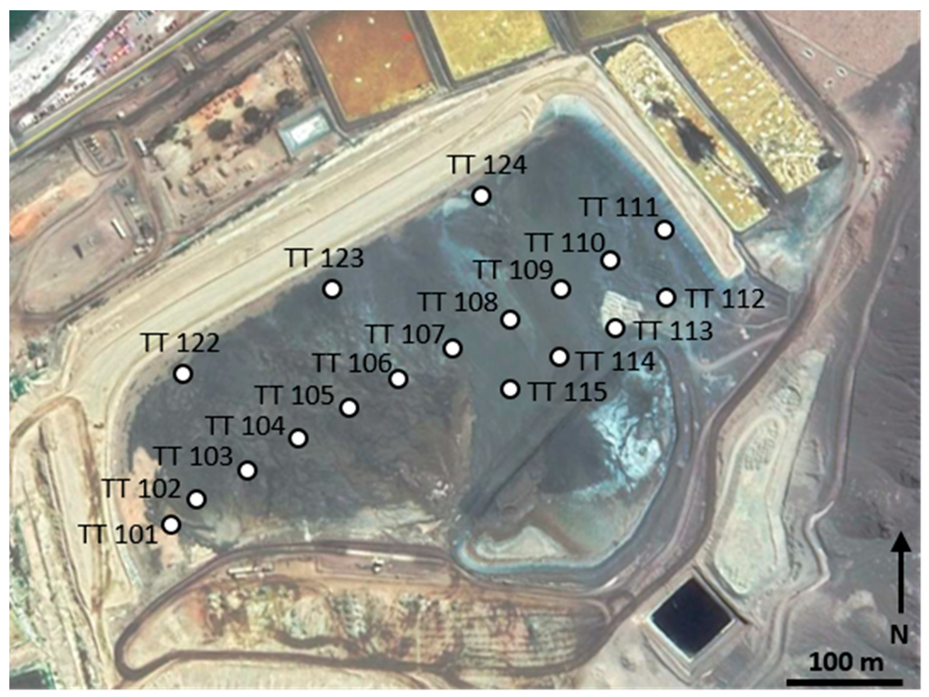
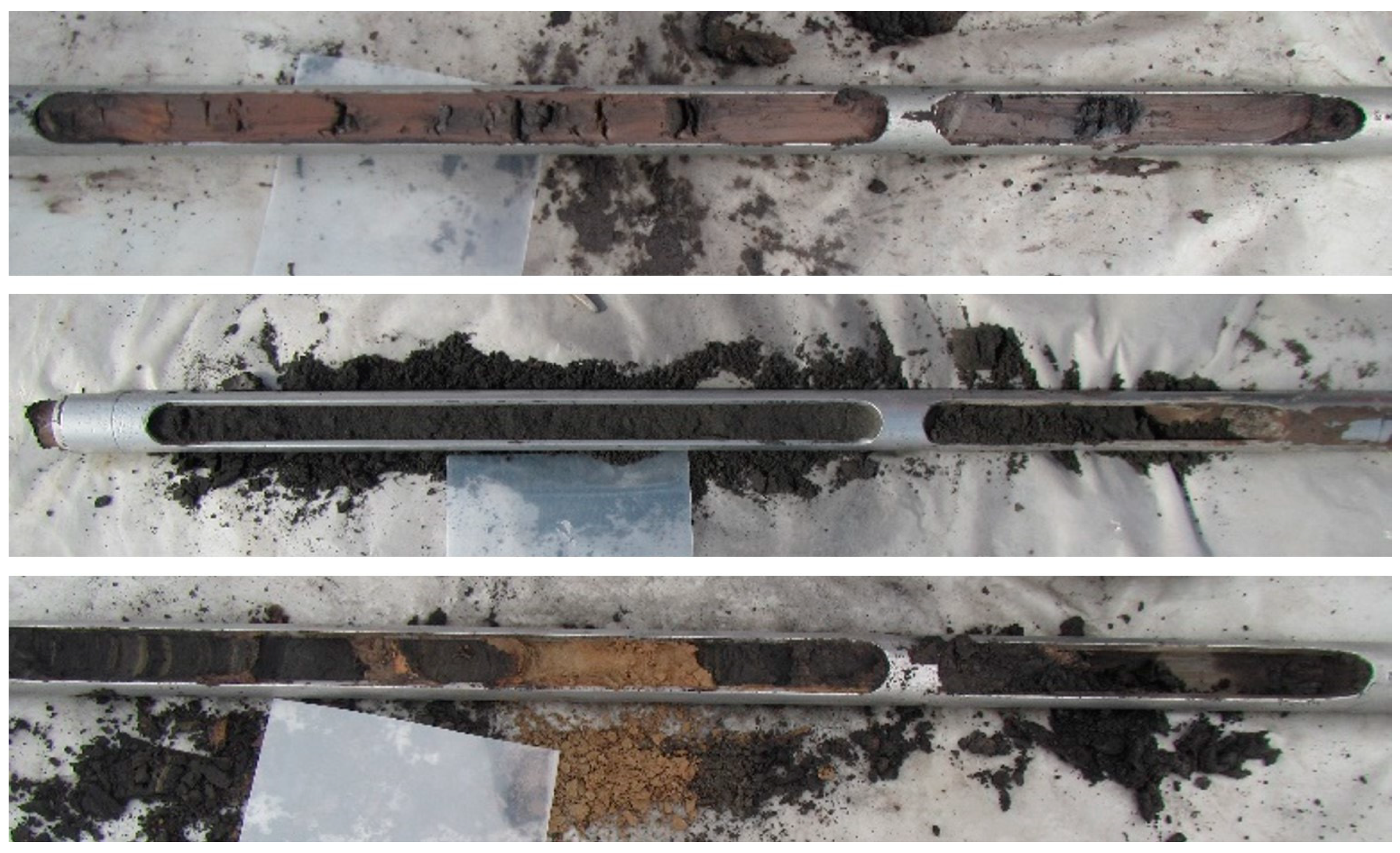
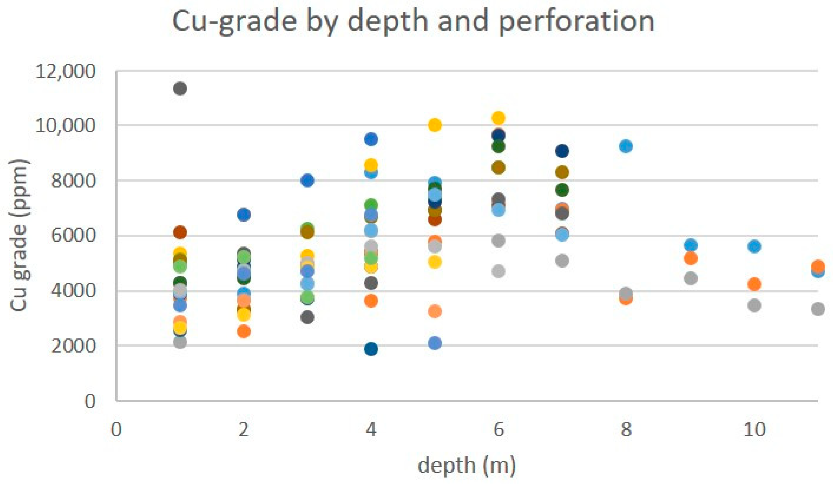
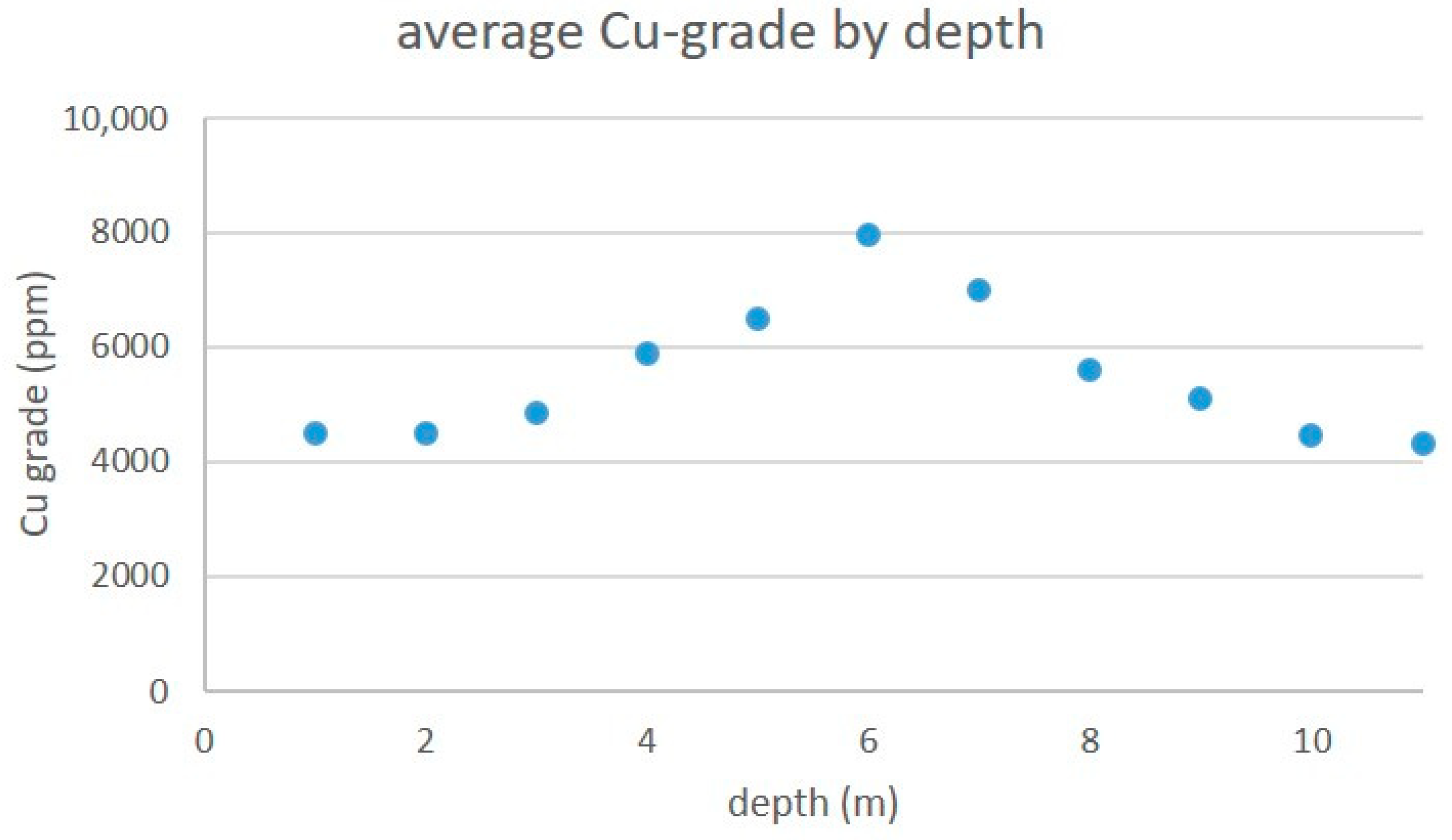
2.1. Tailings Material and Sampling

There are several hundred tailings storage facilities (TSFs) in Chile. For an initial screening to identify the most promising in terms of economic reprocessing, several criteria were evaluated, including age, tonnage, metal grades, type of ore feed (homogeneous or heterogeneous), possible by-products, possible pollutants, ownership, and infrastructure (amongst others). The most challenging in the selection of a TSF is the legal aspect or the simple question: “Do I get the permission to sample on the TSF?” As the project is a collaboration of BGR and a state organization (SERNAGEOMIN), we had access to the tailings of the state owned company ENAMI (Empresa Nacionál de Minería, Santiago de Chile, Chile). As this company buys ore from different small and medium scale enterprises, the ore feed is heterogeneous, which is an advantage for reprocessing, as the flotation cannot be optimized for all mines. Therefore, we first sampled tailings of ENAMI in Ovalle and of some companies close to Ovalle and afterwards tailings of ENAMI in Taltal and of some companies close to Taltal. Due to confidentiality, we cannot name the TSFs. After finishing the sampling, it turned out that the TSF of ENAMI in Taltal (Figure 1) was the most promising in terms of copper grade and possible by-products, in this case magnetite. In order to generate a pilot experiment, the project focused on this relatively small sized TSF of 2 M t. The tailings site contained as main mineral species magnetite (around 20 wt.% of the tailings) and could also be considered copper rich (0.56%). During the construction phase especially of small TSFs, the tailings are size-classified by hydrocyclones, located at the crest of the embankment. The sand-like underflow of the hydrocyclone is used to raise the embankment and the silt-like overflow is deposited on the beach of the enclosed area [25,26]. As a consequence, inside the tailings bodies, there is a vertical and horizontal gradation of the material, according to the deposition velocity of the tailings particles: the further away from the embankment of the TSF, the finer the particle sizes [5,27]. The coarse-sized fraction was usually of black to grey colour and the fine-grained clayish material was either black, reddish or brownish (Figure 2 top and centre). Samples with a high content of clayish material tend to have higher copper grades, compared to black magnetite rich sandy layers. In some samples that are taken from inside of the settling zone of the TSF, layers (a few cm to 20 cm) of yellowish silt could be observed (Figure 2 bottom). These samples had higher contents of arsenic, up to 250 ppm, compared to the average grade of around 90 ppm. The yellowish silt layers are associated with episodic gold processing, in which gold bearing arsenopyrite-ore was milled and floated or density sorted. The average copper grade of all Taltal samples (130) is 0.56% Cu (0.25–1.1% standard deviation 0.19%) and the average iron content is 26% Fe (13–40% Fe, standard deviation 7%). The copper grade is substantially higher compared to the average copper grade in tailings from the 1930s of 0.33% [4] and far above the average of SERNAGEOMIN’s cadaster of mine tailings (sampling only the first meter), which gives copper grades of 0.27% for inactive and abandoned tailings <10 M t [24]. The investigated TSF was in operation between 1966 and 2015. As the processed sulfidic ore came from different mines, the flotation process could not be optimized. Additionally there is oxide and sulfide ore present in the area of Taltal, meaning that the flotation feed most probably had a certain copper oxide mineral content. These factors lead to a high residual copper grade in the tailings. The sampling carried out using a hand held jackhammer that drove a percussion probe into the tailings. One of the advantages of this handy, low cost equipment is the high mobility to change the position on a tailings and the short assembly time at new locations. A road access on the surface of the dried TSF sites was not necessary, as the dismantled lightweight device could be carried easily. As a hand-held device was used, sometimes a high degree of physical strength was needed to penetrate the tailings crusts and hardpan layers. It was especially laborious to recover the sample cores that were enclosed in the drilling probe after every meter of drilling (the sampling device was one meter long). Due to physical limitations, it was at best possible to drill to a depth of 11 m, but as a compromise of working efficiency, 7 m was taken as the target depth. The operational depth limits also lead to the conclusion that only tailings of small size and shallow depth containing up to a few million tons of material can be investigated using this technology. However, in deeper tailings sites, at least a first overview about the contents of the TSF could be obtained. The magnetite and copper-rich TSF near Taltal was investigated with 18 perforations (Figure 1) with a depth of up to 11 m below the tailings surface. In total, 119 samples (each representing 1 vertical m) were taken for subsequent processing tests. The material consisted of an alternating strata of a fine- and coarse-grained material. The fine-grained tailings fraction looked similar to clay and showed plastic behavior. The coarse-grained tailings fraction showed no plastic behaviour and could be classified as silty sand. Sieving tests showed that the fine-grained material had a grain size of d80 < 60 µm and the coarse-grained material showed d80 < 120 µm (Supplementary Materials Figure S1).
To give a better picture about Cu-grade and grade variation, the Cu-grade is shown by depth and per perforation in Figure 3. There is an increase in copper grade with depth from around 0.45% for the first two meters, up to 0.80% at 5 m depth. Three holes (TT122, TT1223, and TT124) were drilled deeper, at the crest of the embankment. Due to the construction of the TSF, this part is coarser-grained, as hydrocyclones classified the material, using the coarser material to raise the TSF. As only the material from these three drilling locations with relatively coarse material is included into the calculation of the average Cu grade from 7–11 m depth, the average grade is only 0.5% between 9 and 11 m (Figure 4). Although there is a tendency for higher copper grades with depth, the strongest correlation for Cu and Fe grade is given by grain size. The coarse-grained material has an Fe grade of 29% and the fine grained material of only 19%. On the other hand, the Cu grade is 0.7% for the fine (37 samples) material and only 0.5% for the coarse material (82 samples).

2.2. Geochemical and Mineralogical Analysis

The sampled material was first analyzed by X-ray fluorescence analysis (XRF) using Philips PW1480 and PW2400 with Cr and Rh excitation at the Federal Institute for Geosciences and Natural Resources (BGR), Hanover, Germany. The mineralogy was examined using X-ray phase analysis. XRD pattern were recorded using a PANalytical X’Pert PRO MPD Θ-Θ diffractometer (Co-Kα radiation generated at 40 kV and 40 mA), equipped with a variable divergence slit (20 mm irradiated length), primary and secondary soller, diffracted beam monochromator, point detector, and a sample changer (sample diameter 28 mm) at BGR, Hannover, Germany. The samples were investigated from 2° to 75° 2Θ with a step size of 0.03° 2Θ and a measuring time of 3 s per step. For specimen preparation the back loading technique was used. Rietveld refinement of the experimental XRD data was conducted using the software BGMN.

2.3. Magnetic Separation

Magnetic separation of the iron fraction was investigated in two ways. Magnetic separation using a hand magnet (0.1 T) was applied on the sample material before the leaching tests (each 8.5 kg) were carried out. A hand magnet can separate magnetic from non-magnetic material, but tends to carry some non-magnetic minerals into the magnetic fraction. The second approach was to use wet magnetic separation in combination with flotation. In this case, a magnetic separator (Sala at the RWTH Aachen, Germany) 20 cm × 11.6 cm with a magnetic field strength of 0.1 T in a metallurgical laboratory was utilized (internal report, RWTH Aachen, 2018). In general, the magnetic material (mostly magnetite) could be separated from the non-magnetic material, which contained among others the majority of the copper minerals.

2.4. Flotation

In order to produce a copper (pre)concentrate, flotation tests were carried out in the laboratories of the AMD of the RWTH in Aachen. A Denver D-12 flotation cell with a volume of 2.5 L was used. The feed was usually 0.5 kg per test, one time 1 kg and one time 1.4 kg. The solid content was 17% for 0.5 kg, 29% for 1 kg, and 37.5% for 1.4 kg with an aeration of 3 L/s. For activation, a planetary ball mill (PM 400 from Retsch, at the RWTH Aachen, Germany) was used. A list of chemicals used can be found below in Table 1.
Ten flotation tests were carried out for the processing scheme flotation followed by magnetic separation (see below). The activation time in the mill was 30 s. Afterwards, various combinations of the above-listed chemicals and pH values were tested. For every test, usually 2–3 chemicals in different dosage were added and flotation was carried out for 3 min. Afterwards, 3–5 more flotation steps were carried out for every test and 1–2 chemicals were added and/or pH adjustments was done, in order to produce the optimum pre-concentrate. For the flotation tests in the scheme magnetic separation before flotation, only four flotation tests with the most promising results from the above-mentioned scheme were carried out, using 0.5 kg of tailings for each test.

2.5. Conventional Sulfuric Acid Chemical Leaching

Conventional leaching tests were carried out, in order to study the recovery and kinetics of acidic copper leaching. The leaching experiments were carried out by G.E.O.S GmbH in Halsbrücke, Germany, on behalf of BGR. The solid to liquid ratio was 1:5 and dilute sulfuric acid was used (concentration of 49 g H2SO4/L H2O, corresponding to 5% sulfuric acid). For the combination of leaching and magnetic separation, for each processing test, 8.5 kg of material were used. The material was mixed with 42.5 L of dilute (5%) sulfuric acid for a solid-liquid ratio of 1 kg: 5 L. After 24 h, the leach residues were washed and prepared for wet-magnetic separation. The separation was done using a NdBFe permanent magnet at 0.1 Tesla.
Compared to conventional leaching in copper mining, the acid grade of 5% is elevated. In heap leaching, a lixiviant with a low acid concentration (0.1–0.5%) is usually applied for months or longer periods for economic reasons. In order to obtain a benchmark result for the leaching process, the decision was taken to carry out the leaching test with a stronger lixiviant applied for a time-period of 24 h within an agitated reactor. This should result in the maximum recovery of copper that is technically and economically feasible. The metal grades in the eluate were analyzed using ICP-OES. The recovery was calculated comparing the XRF results of the input sample with the ICP-OES data of the output eluate (leached out copper).

2.6. Methodological Approach Used for the Economic Assessment

For the economic assessment, standard cost models for (I) flotation and (II) agitation cyanide leach for gold from costmine© were used as a basis. For reprocessing of tailings, mining, crushing, and milling are not necessary, reducing opex and capex. For opex and capex, the daily tonnage is of great importance. According to the TSF tonnage, a mill capacity of 500 t/day was chosen. This daily capacity is relatively low, compared to mining projects of similar size, but will keep the capex and thus the project risk low. Assuming a downtime of 20%, the yearly tonnage would be 146,000 t of material, which translates into a project life of 13.7 years.
In the flotation cost model, the opex is subdivided into four categories and the reduction for reprocessing is given in percent after the category: supplies and materials (66% reduction), labor (45% reduction), administration (33% reduction), diverse (33% reduction). The resulting opex for reprocessing is around 50% lower compared to the original cost model. In order not to underestimate the costs, we chose an opex of 60% of the original costs, which is 13.6 USD/t.
The capex in the flotation model is subdivided into 13 categories and the reduction in capex is given in percent after the category. The categories are equipment (55% reduction), installation labor (50% reduction), concrete (70% reduction), piping (20% reduction), structural steel (70% reduction), instrumentation (50% reduction), insulation (50% reduction), electrics (30% reduction), coatings and sealants (80% reduction), mill building (50% reduction), tailings embankment (10% reduction), and working capital (50% reduction). The reduced capex is 9.4 M USD, around 50% of the original capex.
For the agitation cyanide leach model (the only agitation leach model available), the opex in the cost model is subdivided into comminution, agitation cyanide leach, solid-liquid separation, general operation, and administration. The comminution was completely skipped and the costs for agitation cyanide leach were reduced by 50%. The chemicals for copper leaching are cheaper and due to the fast reaction kinetic, fewer or smaller leaching tanks can be used. This justifies a reduction of 50% of the opex for this category. The total opex is reduced by 60% to 16 USD/t.
The capex is subdivided into comminution, agitation cyanide leach, solid-liquid separation, general, engineering and construction management, and working capital. The comminution costs are omitted and the costs for cyanide leach are halved. Far less volume will be needed for tank leaching due to the reaction kinetic, but as stainless steel is needed in an acid environment, costs can only be reduced by 50%. The same reduction is applied to the general costs, engineering and construction management, and working capital, as comminution is not needed and the volume for tank leaching is far smaller for sulfuric acid leaching, compared to cyanide leaching. The capex sums up to 9.3 M USD, 50% of the original capex.

3. Results and Discussion

3.1. Mineralogy

Besides the geochemical data, mineralogical data was used to determine in which minerals Cu and Fe are located. The geochemical data already showed a high Fe content of 26% on average. A first mineralogical analysis using XRD, focusing on the main mineral phases, confirmed these data with a magnetite grade of 22% for the coarse-grained material and 15% for the fine-grained material (Table 2). A more detailed analysis focusing on minor and trace minerals on the homogenized sample material (coarse- and fine-grained) confirmed the main mineral phases and additionally demonstrated the presence of 0.4% of atacamite and 0.2% chalcopyrite (Table 3). These grades would only translate to a copper grade of 0.31% for the TSF. This leads to the conclusion that the copper minerals were underestimated in the mineralogical analysis, or that there are additional phases not detected by XRD. Microscopic analysis gave hints to the presence of chrysocolla (not detected by XRD). Additionally it is possible that soluble copper phases migrated in the tailings and precipitated on grain surfaces or were adsorbed by clay minerals both not detectable by XRD).

3.2. Semi Technical Processing Tests

The elements with the highest product value in the Taltal tailings are copper and iron. Therefore, the approach for tailings reprocessing is focused on these two elements. For the reprocessing of the tailings material, different processing tests (5–10 kg each) were performed, including flotation, magnetic separation, and leaching, which were combined to processing flowsheets (Figure 5). As the processed ore came from various mines and was originally processed via flotation, starting in 1966, there should still be floatable minerals like chalcopyrite in the TSF. Additionally, the region of Taltal is known for oxide ores that are still processed in Taltal. Therefore, collector chemicals for oxides and sulfides were tested (Table 1). Conventional sulfuric acid leaching was tested, in order to evaluate the recovery and reaction kinetics. As a leaching facility is already installed in Taltal, this could make an economic copper recovery process easier, as some processing infrastructure is already available. Density sorting was also tested, but the recoveries for copper were poor and are not discussed here. It would also be possible to apply bioleaching on the tailings. This method can result in high recoveries of >90% [17] under special environments (e.g., temperature). As we knew that a large share of the copper was present as oxides or chloride, we chose only to apply conventional chemical leaching, as a high recovery was achievable at predictable relatively low costs [28].
The objective of the processing tests was to investigate value concentration paths in order to achieve saleable products or intermediate products in an economically efficient way. In total, four concentration paths were investigated (Figure 5).
The aim was to produce a clean, saleable magnetite concentrate and to evaluate whether it is possible to produce a copper (pre)concentrate as the base of a saleable product, or to leach the copper minerals with dilute sulfuric acid.

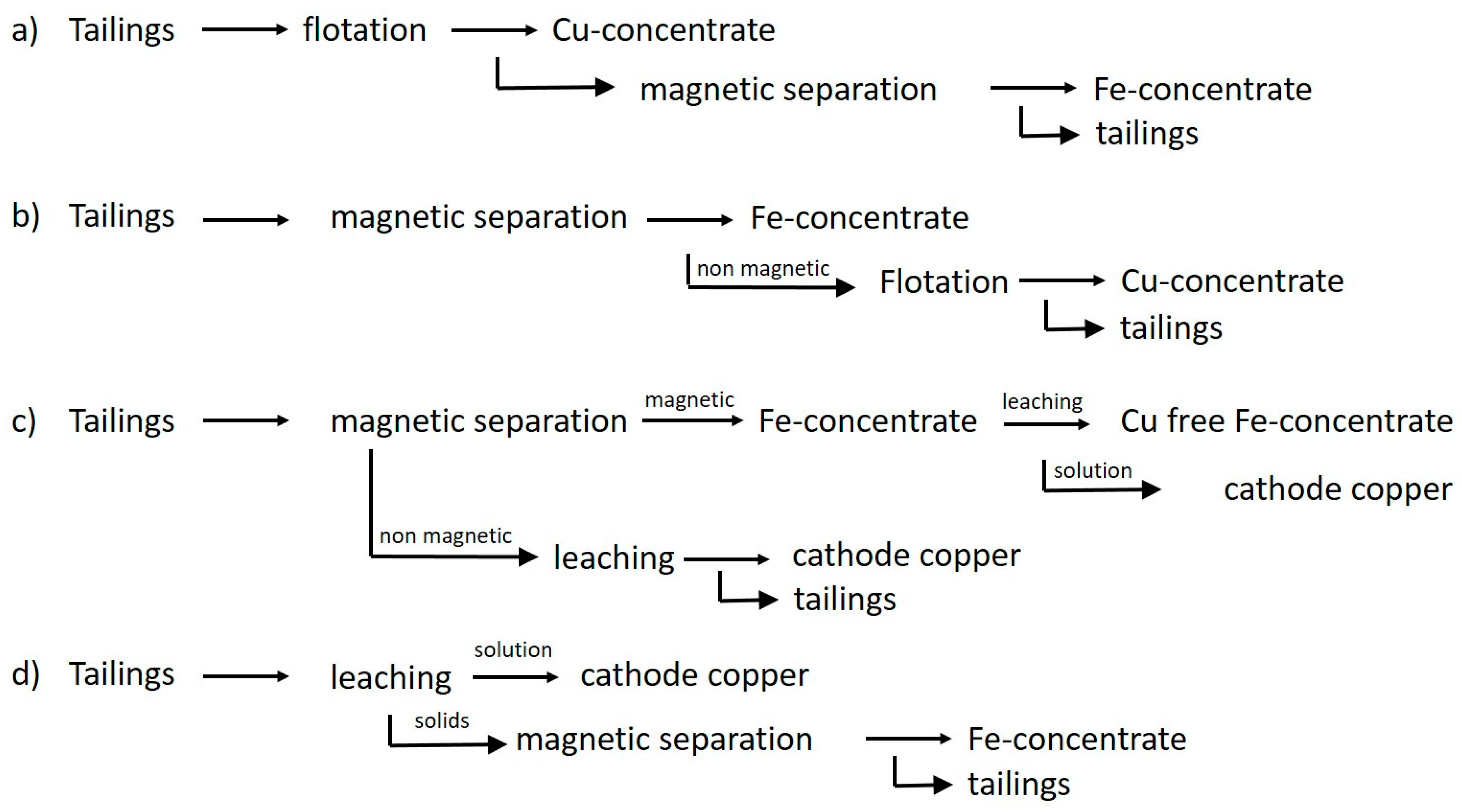
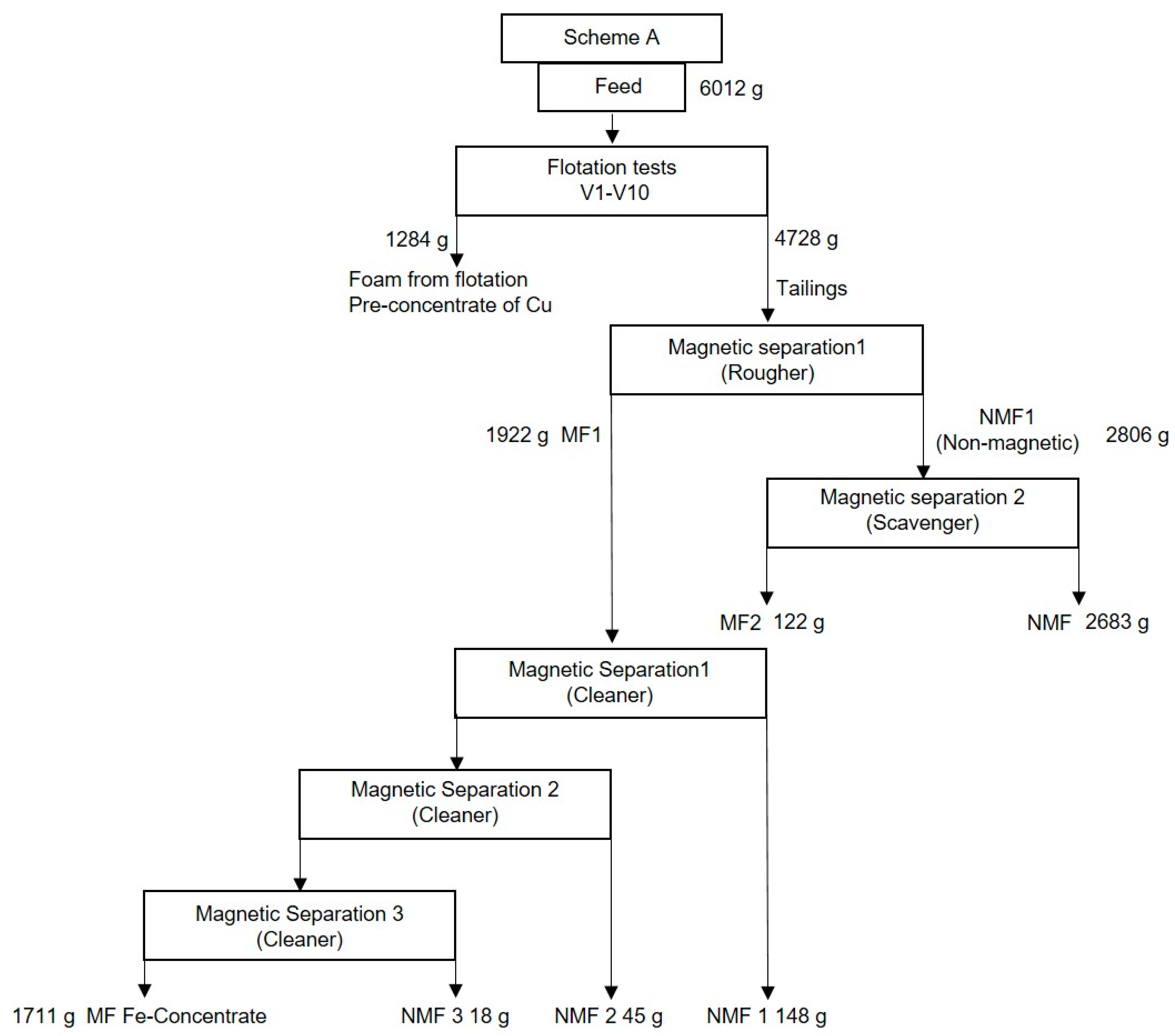
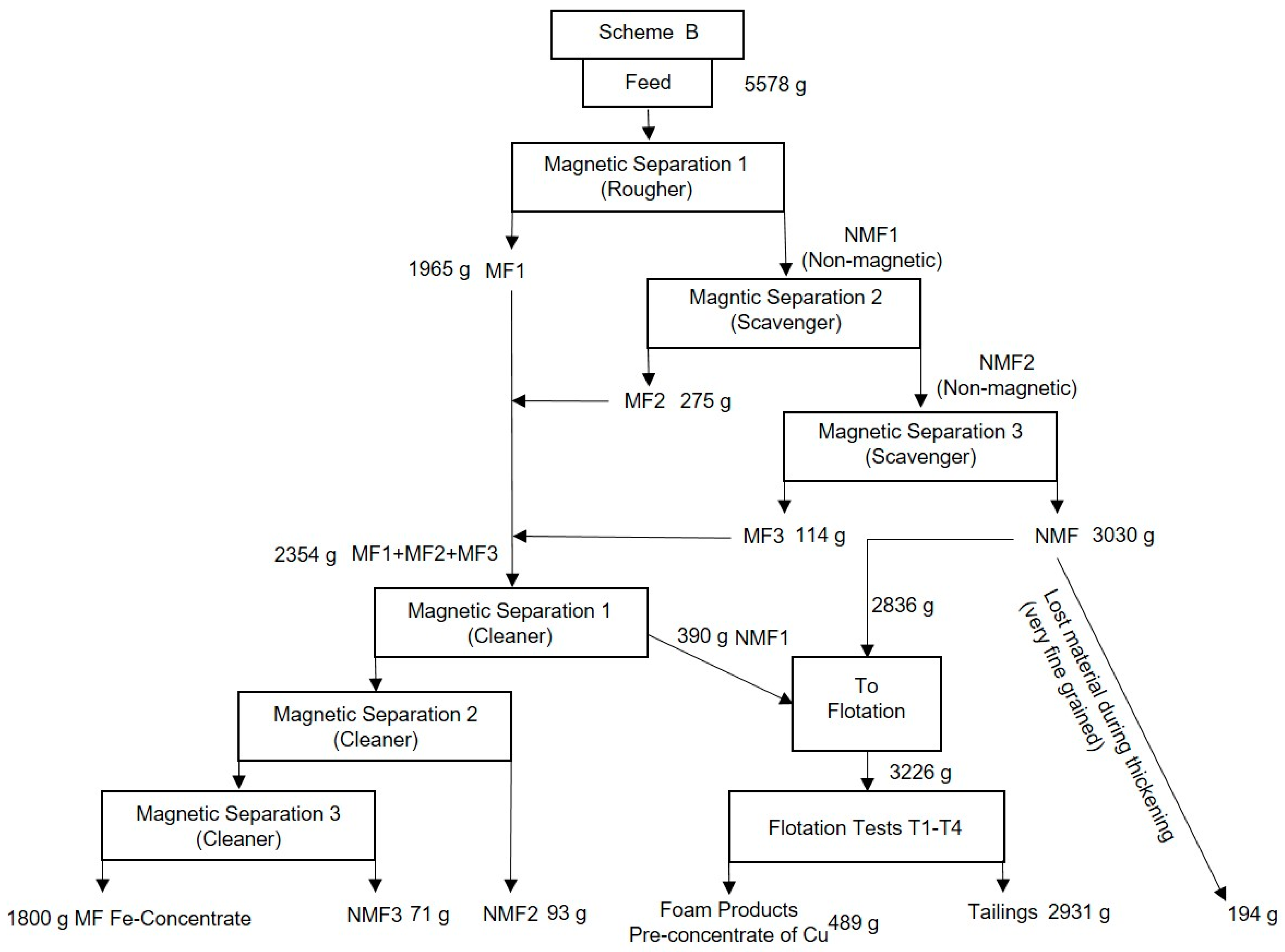
3.2.1. Flotation–Magnetic Separation and Magnetic Separation–Flotation (Figure 5a,b)

As described in Section 3.1, the tailings from Taltal contain significant amounts of copper, as oxides, chlorides, and sulfides, and iron, which is mostly contained in the mineral magnetite. Due to these two value-containing elements, combinations of flotation (oxides and sulfides) followed by magnetic separation and a processing route vice versa were tested (Figure 5a,b). The tests were performed using several kg of material each.
A detailed flowsheet of flotation followed by magnetic separation is given in Figure 6. The tests were carried out according to the description in 2.3. The average recovery was 61% (46–73%) and the average copper grade was 1.8% (1.2–2.2%, excluding Test 10) as shown in Table 4. Recoveries of over 60% for a low grade ore that consists of oxides and sulfides seems quite satisfactory, but the Cu grades of maximum 2.2% for the (pre)concentrates are far too low for a saleable product and would have to be upgraded with an additional method, most probably leaching in an acidic medium, increasing costs and lowering total recovery.
The following magnetic separation (Figure 6) was performed using a magnetic rougher concentration, followed by three magnetic cleaner concentration steps. The result was a concentrate with 60% Fe-content and Fe recovery of 64%. The sulfur content is very low (0.005%), which is a positive fact for selling such a concentrate. Almost 90% of the sulfur is collected in the flotation (pre)concentrate (Table 5).
The second test scheme started with magnetic separation, followed by flotation. The magnetic separation included one rougher, two scavenger steps, and three cleaner separations steps (Figure 7). The recovery of iron into a magnetic concentrate was 74% with an Fe-grade of 60% in the concentrate (Table 6).
Four flotation tests with different flotation chemicals were carried out on the non-magnetic material using the most promising setup and combination of chemicals from the previous tests (tests 6–9 from Figure 5). For each test, around 0.5 kg of tailings material was used (Table 7). The copper recovery of the test was 48–57% of the non-magnetic fraction. The corresponding copper grade was in the range of 1.7–2.4% (average 2.0%). The average copper recovery of this test scheme is only 44%, as there are additional copper losses prior to flotation into the magnetic fraction (Table 6). The copper grade in the (pre)concentrates is similarly low, compared to the scheme of flotation with subsequent magnetic separation. Likewise, it could be possible to subject the (pre)concentrate to an acidic leach process, with the aim to produce saleable copper products, as for example copper cathode or copper chemicals, but the overall recovery of copper is very low.
The advantage of this setup is the higher recovery of Fe into a concentrate, but the copper recovery into a (pre)concentrate is even lower. The relatively high grade of Cu in the Fe concentrate (0.14%) is still far below the restrictions given for several steel grades, e.g., railway steel (0.4%) and some steel used in construction (0.55%) that can be found online [29].

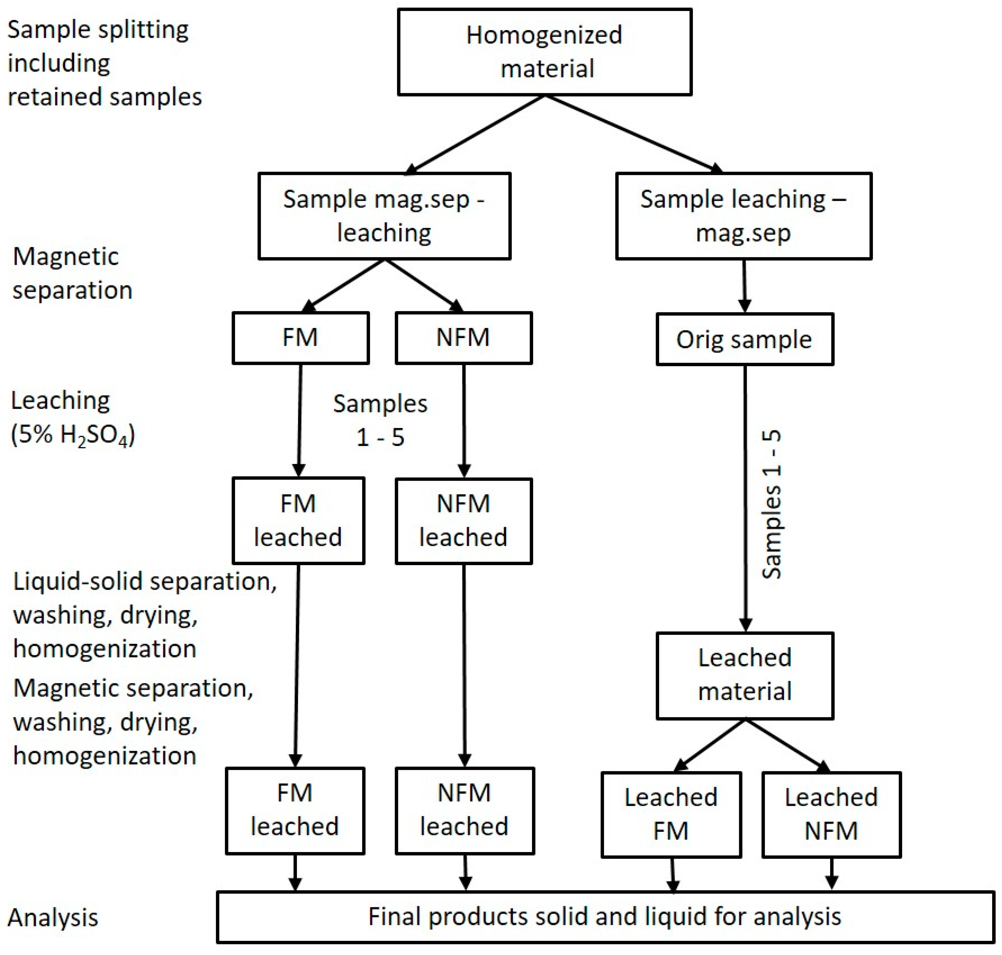
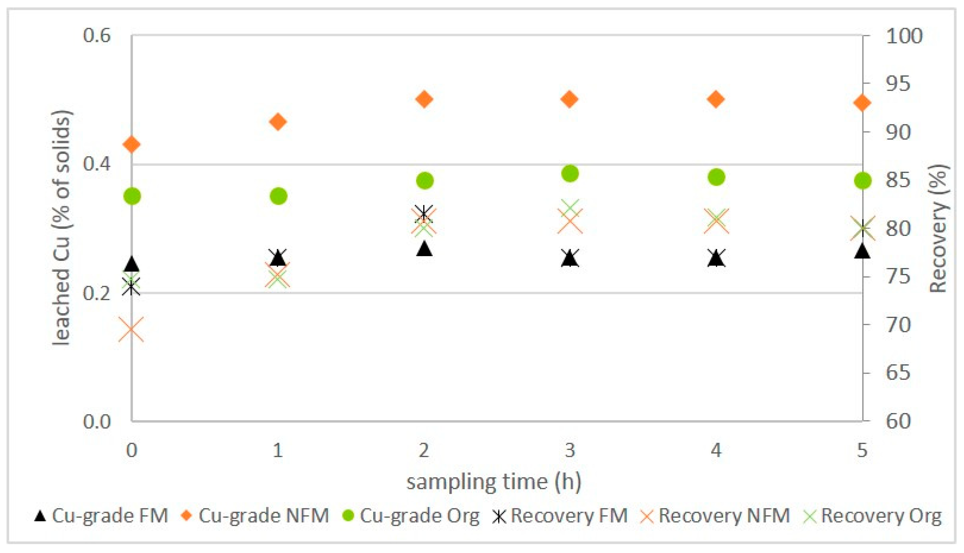
3.2.2. Leaching–Magnetic Separation and Magnetic Separation–Leaching (Figure 5c,d)

The combination of leaching and magnetic separation is schematically shown in Figure 8. Relatively strong sulfuric acid of 5% was used, in order to obtain a maximum value for leaching recovery. Leaching kinetics (Figure 9) are very fast (hours), compared to days in bioleaching [17], at least for the high acid grades applied. From the original (Org) sample material, 70% of Cu could immediately (after 5 min) be leached (Figure 9), as the copper is concentrated in oxide, chloride, or carbonate minerals. After one hour, 77% of the contained copper was already leached. The maximum leaching recovery was 84%. The leaching kinetics and recoveries were similar for the non-ferromagnetic material (NFM) with a recovery of around 80% for both. The gathered Cu bearing solution has a grade of 730 mg Cu/L, probably too low for direct application of solvent extraction.
Magnetic separation of the original, non-leached material resulted in a magnetic fraction (40%) of the material and a non-magnetic fraction (60%). The Fe-grade in the FM fraction was 47%, compared to 26% before the separation. The Fe-grade was higher after leaching (52%), at the expense of SiO2, CaO, and most other major elements. This Fe-content is relatively low, as a marketable iron concentrate should have 62%. The processing tests of flotation combined with magnetic separation resulted in concentrates with Fe-grades of 60% (Table 5 and Table 6). The larger portion of the Fe-concentrate (40% compared to 28–33% in Table 5 and Table 6) results in a lower Fe-grade of only 52%, as the separation worked poorer.
When applying magnetic separation after leaching (Figure 5d), the Fe grade in the magnetic fraction was only 43%, not encouraging, as this concentrate is not marketable. The reason for the substantially lower Fe grades might be connected to different equipment used for the magnetic separation, including missing cleaner steps. For the leaching recovery, it is not important if leaching or magnetic separation is applied first. In contrast, it does play a role in the quality of the magnetic separation, whether magnetic separation is done before leaching, or afterwards, as leaching can decrease grainsize, which has a negative effect on magnetic separation.

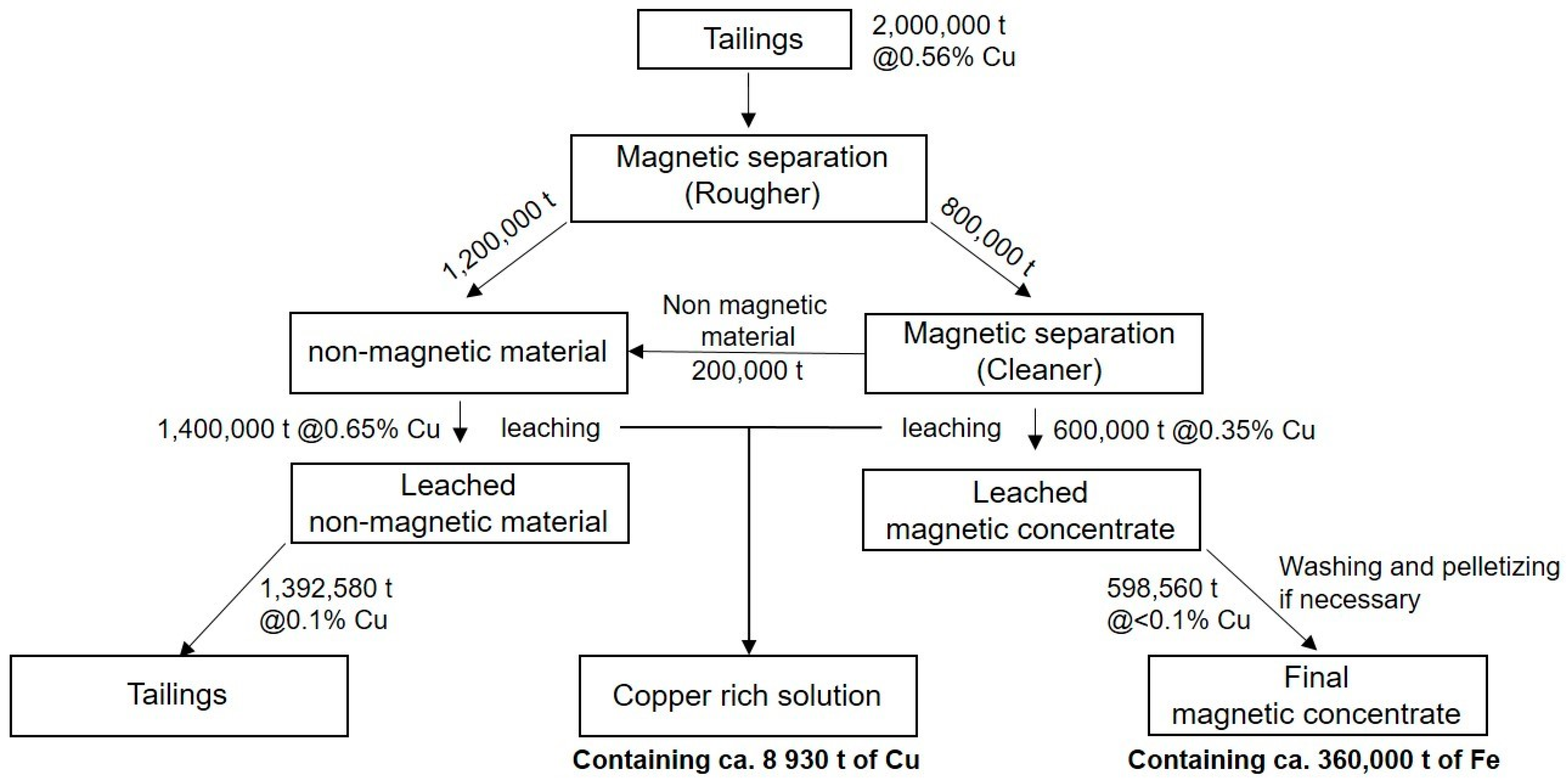
3.3. Introduction of Adjusted Cost Models

In an industrial scale processing facility, usually lower acid grades of 0.1–0.5% are applied in combination with a longer reaction time. A lower acid grade reduces the grade of undesired elements in solution and therefore reduces the acid consumption, as less material is dissolved (both not tested in this paper). Considering the realized semi-technical tests for reprocessing in this paper, the most promising processing option for the production of a magnetite concentrate and copper intermediates is as follows (Figure 10):
  • Magnetic separation into FM and NFM fraction, including magnetic cleaner steps
  • Separate leaching of the FM and NFM material in stirred tank or horizontal rotary reactor with dilute sulfuric acid (below 5%) in continuous or batch mode (for several hours)
  • Final production of an Fe-concentrate (Cl-, S-, P- and Cu-grades could be an issue)
  • Hydrocyclone and/or settling to separate solids and liquids (Cu-rich solution)
  • Washing of solids to remove rests of copper (dilute Cu-solution)
  • Deposition of the NFM fraction (finer-grained than original tailings material)
  • Further concentration and cleaning of Cu-solution to produce intermediate products, or cathodes by electrowinning
In step 7 above, a further concentration and cleaning of the Cu solution is mentioned as the copper grade of the solution is only 730 mg Cu/L. A combination of the relatively low-grade solution with the higher grade solution of the nearby heap leaching facility in Taltal could be possible. Another option would be to recirculate the solution or to increase the solid-liquid ratio, to increase the copper grade. Afterwards, solvent extraction could be applied. It would also be possible to use a different technique like ion exchange, in order to adsorb the copper on a resin, to produce a high grade copper solution on which electrowinning could directly be applied on.
In the following discussion of the cost models, the presented scheme in Figure 10, as well as flotation are discussed, as flotation is a possible technique for reprocessing many TSFs. Flotation can be applied for economic reprocessing, but also to reduce sulfide grades and minimize acid rock drainage.
For the economic assessment, a revenue of 65 USD/t of magnetite concentrate was assumed. The average price over the last five years was 72 USD/t for 62% Fe iron ore concentrate (cost freight China), but there are still uncertainties about production costs and quality of the concentrate. Therefore, a more conservative revenue is assumed. For copper cathode, the average price in the last five years was around 5500 USD/t, which is used for the economic evaluation. In order to process the tailings deposit of 2,000,000 t, a 500 t/d capacity processing plant is supposed to be a realistic match, in order to minimize the preproduction expenditures. Larger processing facilities would improve the long-term economics of the project [22,30], but also increase the economic project risks. The annual capacity is assumed to be 146,000 t (see Section 2.5). It is generally possible to produce marketable copper concentrates from tailings. This can be seen in the concentrates of Minera Valle Central, although the size of the operation is several orders of magnitude larger compared to the tailings described here. Reference [10] also demonstrates the possibility to produce a concentrate with a copper grade of 19 % from fresh tailings or almost fresh tailings at low cost at a large industrial scale (150,000 t/d). The processing costs would be 5.6 USD/t, taking the data from their publication (Labor, Energy, Chemicals). As the Taltal TSF only contains around 2 M t of material, substantially higher costs have to be assumed.
When reprocessing tailings, a hydraulic transport of the slurried tailings to the plant or transport via truck, an activation grinding, and a desliming classification of the tailings has to be done. According to [10], desliming is possibly not necessary as in certain cases, ultrafine particles can also be floated and even increase the recovery.

3.4. Comparison of Cost Models and NPV

The given capex and opex from costmine© for a flotation processing plant of 500 t/d is 22 USD/t and an investment of around 15.7 Mio USD. As no crushing is needed and if milling only to a very small amount, these costs can be subtracted, leading to processing costs of around 13.2 USD/t and investment costs of 9.4 M USD (Section 2.5 and Table 8). These costs are too high to carry out economic reprocessing in Taltal (Table 9 and Table 10). To cover the operating costs of 13.2 USD/t, at a copper price of 5500 USD/t, the recoverable copper grade has to be 0.24%. To refinance the capex over 10 years, additional 170 t of copper (around 940,000 USD) would have to be extracted annually and marketed without deduction, equivalent to additional 0.12% recoverable. This results in a minimum recoverable copper grade of 0.35%, just to cover capex and opex. The opex of the adopted cost model for flotation is more than two times higher, compared to [10], but these authors worked at a processing plant with a capacity of 150,000 t/d, which is the yearly processing capacity, chosen in our cost model. Based on these data, it seems difficult to achieve an economic reprocessing for copper in small tailings dams. In addition to the 0.35% of recoverable copper needed to refinance opex and capex, discounted cash flow (10%) is usually applied, leading to even higher needed recoveries. Furthermore, a net smelter return (NSR) for transport, treatment, and refining the concentrate (deductions of 10–20%) has to be subtracted from the metal value. Nevertheless, the cost estimation can be a basis for rules of thumb, when relatively small tailings have to be reprocessed for environmental reasons, e.g., to reduce acid drainage.
For the required magnetic separation, only a very rough cost estimation was possible, since this processing method is not part of the standard cost models of costmine©. The opex is dominated by freight costs to the next harbor facility. Using the rule-of-thumb-costs for truck transport of 10 US cent per ton and mile [22], additional freight costs of around 15.0 USD/t for the transport of the magnetite concentrate to the next harbor (150 miles to Caldera) have to be added to the plant operation costs. The operation costs consist of the costs for magnetic separation, cleaner separation, thickening, drying, and equipment and were estimated at about 5 USD per processed ton of tailings. The required investment for the plant has been estimated to about 1 M USD. The total costs for the recycling of 2 M t of tailings, including transport to the next harbor, would be in the range of 20 M USD (around 10 USD/t), depending on the amount of concentrate that has to be transported. According to the model costs and the calculated revenue (Table 9 and Table 10), magnetic separation would result in revenues that are around two times higher, compared to the costs.
The results from the magnetic separation are very encouraging in both processing schemes, although the copper grade and other deleterious elements have to be examined in more detail. This is particularly valid for the chloride grade, which could not be analyzed by XRF. The origin of the chloride is seawater, which is frequently used in the dry coastal areas for processing. Nevertheless, if saleable, the magnetite concentrate would give a very profitable product (Table 9 and Table 10). In case of flotation, the concentrates do not pay the costs for processing and investment. Even if it were possible to reduce the costs for investment by purchasing used equipment, flotation does not seem to be an appropriate processing technique, as the concentrate grades are far below any saleable product. The only reason to do flotation would be a desulfurization of the tailings, to prevent acid drainage, as up to 90% of the sulfur can be recovered in the flotation products.
Next to flotation, heap leaching is the second most common processing method for copper ores [12]. Due to the fine-grained tailings material, heap leaching is difficult to apply, as acid tolerant binders to agglomerate the material are limited [31]. Therefore, agitation tank leaching would have to be carried out, which is relatively expensive in terms of capex and opex. Examples for costs can be found in various feasibility studies, for example the Raventhorpe project in Australia, which is slightly larger (two times) compared to the investigated tailings in this paper [32]. The reaction kinetics for leaching are very fast, as almost all of the leachable copper was in solution after 2 h (Figure 9), at least at an admittedly high acid concentration of 5% H2SO4. Similar kinetics were also described by [33]. The recovery of approximately 80% for the 2 M t of tailings with an average copper grade of 0.56% (Table 9 and Table 10 refer to the coarse-grained material only) leads to around 8900 t of recoverable copper with a metal value of 49.1 M USD.
As a basis for a rough estimation of capex and opex, the agitated cyanide tank-leaching model for Gold from costmine© was chosen and adjusted (Table 8). The new capex is 9.3 M USD (for new equipment)—50% of the model capex—and the opex is 16 USD/t for tailings, 60% less, compared to the model opex. This results in total costs for the processing of about 41.3 M USD. Compared to the calculated revenue of 49.1 M USD, the reprocessing of the tailings would result in a small profit (Table 11). The opex data of 16 USD/t is equivalent to 0.29% of leached copper (at a price of 5500 USD/t). Additionally, 0.12% of Cu has to be recovered to refinance the capex of 9.3 M USD over 10 years. This leads to a total grade of 0.41% that has to be recovered just to cover the costs. The 2 M t would be processed in 13.7 years (146,000 t/a) and 652 t of Cu would be produced per year (8930/13.7), leading to a positive cash flow of 7.8 M USD per year (5500 USD/t Cu) minus investment. A dynamic model using discounted cash flow (10%) results in an NPV of 0.2 M USD. These calculations are prone to changes in copper price and recovery/recoverable grade. A price variation of 10 % for copper (500 USD/t of copper) results in changes of 2.5 M USD in the NPV and thus a negative NPV of −2.3 M USD, or an NPV of 2.7 M USD in a positive scenario. Taking the copper price of December 2020 (7700 USD/t), we would get an NPV of 11.1 M USD, but it must be avoided to use these extremely positive assumptions as prices are cyclical. Similar variations of around 2.8 M USD can be seen when we introduce a scenario with a grade variation of 10% from the original grade of 0.56%. A grade reduction leads to a negative NPV of −2.1 M USD and a higher grade of 0.61% leads to a far more positive result of 3 M USD. A double negative (price and grade) scenario would lead to a devastating NPV of −4.7 M USD and a double positive scenario would lead to relatively promising NPV of 5.7 M USD.
The cash flow calculation for the magnetite is clearly positive. The annual cash flow is 1.46 M USD, which sums up to an NPV of 10 M USD using a 10% discount rate, quite high for the amount invested. There are similar changes to the economies, when applying positive or negative scenarios for recovery and prices, but the NPV will always be positive. The biggest risk for magnetite is the production of a marketable concentrate and to enter into an offtake agreement for such low volume.
Mobile processing plants are also discussed in the literature, especially for tailings of relatively small (<100,000 m3) volume [34] or placer deposits [35]. Other authors [36] supposed such a strategy for a TSF of similar size to Taltal. Nevertheless, it has to be considered that a project life of almost 14 years most probably leads to permanently installed technology, but it should be considered that at least parts of the processing plant are built in a way to use them for other TSFs in the region afterwards, especially for the production of Fe-concentrates.

4. Conclusions

Cost models, including an approximate estimation of the capacity of the processing plant offer the opportunity for a rough economic assessment in an early project stage, before cost-intensive processing tests in a pilot plant scale are conducted. Additionally, this allows comparing projects of different grade and different tonnage. Larger scale processing tests can be carried out on the most promising projects, to check the results of the tests, in order to proceed closer to an industrial scale plant. Early stage cost estimations for tailings reprocessing show that opex can be reduced by 40% and capex by 50% for a flotation plant with a capacity of 500 t/d. The opex is reduced to 13.2 USD/t and the capex is reduced to 9.4 M USD. Used equipment would further reduce costs. To cover opex and capex, without discounted cash flow and neglecting the NSR, a minimum copper grade of 0.35% has to be extracted from the tailings, too much for the investigated example.
In case of a high content of copper oxides in the tailings, leaching with dilute sulfuric acid can be a feasible alternative. The adopted cost-model of cyanide gold leaching resulted in capex of 9.3 M USD and opex of 16 USD/t. This is a reduction of 60% of the opex and 50% of the capex of the model. The advantage of leaching in this case is the high recovery of 80% and the option to produce copper cathode from the pregnant leach solution instead of a (pre)concentrate that needs further treatment. To cover opex and capex, without discounting the cash flow, a copper grade of 0.41% has to be extracted from the tailings. When applying a discount rate of 10%, the extracted grade has to be around 0.44% Cu, to get an NPV of 0.
The disadvantage in leaching is that acids reduce the grain size of the material. This may cause some issues for re-deposition that would have to be investigated in more detail in a pilot-plant study.
In the case of the Taltal tailings, the most economical processing method is the concentration of magnetite. The presented semi-technical scale tests result in a recovery of 30% of the total material (600,000 t) to a magnetic concentrate of around 60% Fe-grade (value around 39 M USD). As opex and capex are low for magnetic separation, the magnetite in the tailings is the most profitable commodity with an NPV (10%) of around 10 M USD.
In Chile, there are around 50 tailings with 25 M t and an Fe2O3 grade >30% that have a high potential to produce Fe-concentrates and another around 100 Mio. t close to Copiapó, where similar deposits to Taltal are mined with a potential to produce Fe-concentrates.

Supplementary Materials

The following are available online at https://www.mdpi.com/2075-4701/11/1/103/s1, Figure S1: Grain size distribution of the sample material that was macroscopically divided into “coarse” and “fine” grained.

Author Contributions

Conceptualization, M.D. and H.M.; methodology, M.D.; validation, M.D., M.G., H.M., and F.H.; formal analysis, F.H. and M.D.; investigation, M.D., F.H., and M.G.; writing—original draft preparation, M.D.; writing—review and editing, M.D., F.H., H.M., and M.G.; All authors have read and agreed to the published version of the manuscript.

Funding

This research received no external funding.

Institutional Review Board Statement

Not applicable.

Informed Consent Statement

Not applicable.

Data Availability Statement

The data presented in this study are available in the article.

Acknowledgments

As part of the commodity partnership agreed between Chile and Germany, the Federal Institute for Geosciences and Natural Resources (BGR, Hannover, Germany) has initiated a project together with the Chilean Geological survey SERNAGEOMIN to evaluate the economic potential for reprocessing/recycling of mining residues with the focus on copper and other elements of value. M.D. wants to thank SERNGEOMIN for the excellent cooperation, including sampling, discussion, and logistics. Special thanks go to OR and B. Processing tests were carried out by RWTH Aachen and G.E.O.S. Ingenieurgesellschaft mbH.

Conflicts of Interest

The authors declare no conflict of interest.

References

  1. Drobe, M. Vorkommen und Produktion Mineralischer Rohstoffe—Ein Ländervergleich. 2020. Available online: https://www.bgr.bund.de/DE/Themen/Min_rohstoffe/Downloads/studie_Laendervergleich_2017.pdf?__blob=publicationFile&v=7 (accessed on 1 July 2020).
  2. Lottermoser, B. Mine Wastes: Characterization, Treatment, and Environmental Impacts, 3rd ed.; Springer: Berlin, Germany, 2010. [Google Scholar]
  3. SERNAGEOMIN. Anuario de la Minería de Chile 2019. Available online: https://www.sernageomin.cl/pdf/anuario_2019_act100720.pdf (accessed on 14 July 2020).
  4. Alcalde, J.; Kelm, U.; Vergara, D. Historical assessment of metal recovery potential from old mine tailings: A study case for porphyry copper tailings, Chile. Miner. Eng. 2018, 127, 334–338. [Google Scholar] [CrossRef]
  5. Nikonow, W.; Rammlmair, D.; Furche, M. A multidisciplinary approach considering geochemical reorganization and internal structure of tailings impoundments for metal exploration. J. Appl. Geochem. 2019, 104, 51–59. [Google Scholar] [CrossRef]
  6. Araya, N.; Kraslawski, A.; Cisternas, L.A. Towards mine tailings valorization: Recovery of critical materials from Chilean mine tailings. J. Clean. Prod. 2020, 263, 121555. [Google Scholar] [CrossRef]
  7. Giurco, D.; Prior, T.; Mudd, G.; Mason, L.; Behrisch, J. Peak Minerals in Australia: A Review of Changing Impacts and Benefits; Department of Civil Engineering, Monash University: Clayton, Australia, 2010; Available online: https://opus.lib.uts.edu.au/bitstream/10453/31155/1/2009003150OK.pdf (accessed on 15 September 2020).
  8. Gordon, R.B. Production residues in copper technological cycles. Resour. Conserv. Recycl. 2002, 36, 87–106. [Google Scholar] [CrossRef]
  9. Evdokimov, S.I.; Evdokimov, V.S. Metal recovery from old tailings. J. Min. Sci. 2014, 50, 800–808. [Google Scholar] [CrossRef]
  10. Yin, Z.; Sun, W.; Hu, Y.; Zhang, C.; Guan, Q.; Wu, K. Evaluation of the possibility of copper recovery from tailings by flotation through bench-scale, commissioning, and industrial tests. J. Clean. Prod. 2018, 171, 1039–1048. [Google Scholar] [CrossRef]
  11. Mackay, I.; Videla, A.R.; Brito-Parade, P.R. The link between particle size and froth stability—Implications for reprocessing of flotation tailings. J. Clean. Prod. 2020, 242, 118436. [Google Scholar] [CrossRef]
  12. Schippers, A.; Hedrich, S.; Vasters, J.; Drobe, M.; Sand, W.; Willscher, S. Biomining: Metal Recovery from Ores with Microorganisms. In Geobiotechnology I. Advances in Biochemical Engineering/Biotechnology; Schippers, A., Glombitza, F., Sand, W., Eds.; Springer: Berlin/Heidelberg, Germany, 2013; Volume 141, pp. 1–47. [Google Scholar] [CrossRef]
  13. Xie, Y.; Xu, Y.; Yan, L.; Yang, R. Recovery of nickel, copper and cobalt from low-grade Ni-Cu sulfide tailings. Hydrometallurgy 2005, 80, 54–58. [Google Scholar] [CrossRef]
  14. Olson, G.J.; Brierley, C.L.; Briggs, A.P.; Calmet, E. Biooxidation of thiocyanate-containing refractory gold tailings from Minacalpa, Peru. Hydrometallurgy 2006, 81, 159–166. [Google Scholar] [CrossRef]
  15. Schippers, A.; Nagy, A.A.; Kock, D.; Melcher, F.; Gock, E.-D. The use of FISH and real-time PCR to monitor the biooxidation and cyanidation for gold and silver recovery from a mine tailings concentrate (Ticapampa, Peru). Hydrometallurgy 2008, 94, 77–81. [Google Scholar] [CrossRef]
  16. Marrero, J.; Coto, O.; Goldmann, S.; Graupner, T.; Schippers, A. Recovery of nickel and cobalt from laterite tailings by reductive dissolution under aerobic conditions using Acidithiobacillus species. Environ. Sci. Technol. 2015, 49, 6674–6682. [Google Scholar] [CrossRef] [PubMed]
  17. Falagán, C.; Grail, B.M.; Johnson, D.B. New approaches for extracting and recovering metals from mine tailings. Miner. Eng. 2017, 106, 71–78. [Google Scholar] [CrossRef]
  18. Edraki, M.; Baumgartl, T.; Manlapig, E.; Bradshaw, D.; Franks, D.M.; Moran, C.J. Designing mine tailings for better environmental, social and economic outcomes: A review of alternative approaches. J. Clean. Prod. 2014, 84, 411–420. [Google Scholar] [CrossRef]
  19. Dold, B.; Fondbote, L. Element cycling and secondary mineralogy in porphyry copper tailings as a function of climate, primary mineralogy, and mineral processing. J. Geochem. Explor. 2001, 77, 3–55. [Google Scholar] [CrossRef]
  20. S&P Global. SNL Database. Commercial Online-Databank. Available online: https://platform.marketintelligence.spglobal.com/web/client#dashboard/metalsAndMining (accessed on 14 July 2020).
  21. Lottermoser, B.G. Recycling, reuse and rehabilitation of mine wastes. Elements 2011, 7, 405–410. [Google Scholar] [CrossRef]
  22. Wellmer, F.W.; Dalheimer, M.; Wagner, M. Economic Evaluations in Exploration, 3rd ed.; Springer: Berlin/Heidelberg, Germany, 2008; p. 250. [Google Scholar] [CrossRef]
  23. Wellmer, F.W.; Drobe, M. A quick estimation of the economics of exploration projects—Rules of thumb for mine capacity revisited—The input for estimating capital and operating costs. Bol. Geol. Min. 2019, 130, 7–26. [Google Scholar] [CrossRef]
  24. SERNAGEOMIN. Datos de Geoquímica de Depósitos de Relaves de Chile (actualización: 13/01/2020). Available online: https://www.sernageomin.cl/datos-publicos-deposito-de-relaves/ (accessed on 15 June 2020).
  25. Vick, S.G. Planning, Design, and Analysis of Tailings Dams; Wiley: New York, NY, USA, 1983; p. 369. [Google Scholar]
  26. Bussière, B. Colloquium 2004: Hydrogeotechnical properties of hard rock tailings from metal mines and emerging geoenvironmental disposal approaches. Can. Geotech. J. 2007, 44, 1019–1052. [Google Scholar] [CrossRef]
  27. Blight, G.; Bentel, G. The behaviour of mine tailings during hydraulic deposition. J. S. Afr. Inst. Min. Metall. 1983, 83, 73–86. [Google Scholar]
  28. Long, K.R.; Singer, D.A. A Simplified Economic Filter for Open-Pit Mining and Heap-Leach Recovery of Copper in the United States. In USGS Open-File Rep.; 2001; 01-218. Available online: https://pubs.usgs.gov/of/2001/0218/pdf/of01-218.pdf (accessed on 15 September 2020).
  29. b2bmetal (2020). Online Metal Marketplace with Requirements for Several Steel Grades Including Mechanical Properties, Chemical Composition and Grade Equivalents. Available online: http://www.b2bmetal.eu/en/pages/index/index/id/141/ (accessed on 20 November 2020).
  30. Long, K.R. A Test and Re-Estimation of Taylor’s Empirical Capacity-Reserve Relationship. Nat. Resour. Res. 2009, 18, 57–63. [Google Scholar] [CrossRef]
  31. Dhawan, N.; Sadegh Safarzadeh, M.; Miller, J.D.; Moats, M.S.; Rajaman, R.K. Crushed ore agglomeration and its control for heap leach operations. Miner. Eng. 2013, 41, 53–70. [Google Scholar] [CrossRef]
  32. ACH Minerals 2016. Appendix 2: Capital and Operating Cost Estimate—GR Engineering Services. Available online: https://consultation.epa.wa.gov.au/seven-day-comment-on-referrals/ravensthorpe-gold-copper-project/supporting_documents/CMS16331%20%20Referral%20%20Appendix%202%20Captial%20and%20Operating%20Cost%20Estimate.pdf (accessed on 29 July 2020).
  33. Conić, V.; Stanković, S.; Marković, B.; Božić, D.; Stojanović, J.; Sokić, M. Investigation of optimal technology for copper leaching from old flotation tailings of the copper mine Bor (Serbia). Metall. Mater. Eng. 2020, 26, 209–222. [Google Scholar] [CrossRef]
  34. Kuhn, K.; Meima, J.A. Characterization and Economic Potential of Historic Tailings from Gravity Separation: Implications from a Mine Waste Dump (Pb-Ag) in the Harz Mountains Mining District, Germany. Minerals 2019, 9, 303. [Google Scholar] [CrossRef] [Green Version]
  35. Nevskaya, M.A.; Seleznev, S.G.; Masloboev, V.A.; Klyuchnikova, E.M.; Makarov, D.V. Environmental and Business Challenges Presented by Mining and Mineral Processing Waste in the Russian Federation. Minerals 2019, 9, 445. [Google Scholar] [CrossRef] [Green Version]
  36. Figueiredo, J.; Vila, M.C.; Góis, J.; Pavani Biju, B.; Futuro, A.; Martins, D.; Dinis, M.L.; Fiúza, A. Bi-level depth assessment of an abandoned tailings dam aiming its reprocessing for recovery of valuable metals. Miner. Eng. 2019, 133, 1–9. [Google Scholar] [CrossRef]
Figure 1. TSF near Taltal (Google Earth) with drilling locations. The tailings have their maximum thickness (15 m) in the northern area (TT 122 to TT 124), where samples were taken up to a depth of 11 m and is thinning to the SSW. There are no drilling spots SE and SW of TT 115, as the tailings pond became very shallow (below 4 m).
Metals 11 00103 g001
Figure 2. Probe with sample material from the Taltal tailings. Top: reddish copper rich clay. Center: dark magnetite rich sandy material. Bottom: yellowish layer probably from episodic gold processing (direct information of the owner of the tailings). Length of probe 1 m.
Metals 11 00103 g002
Figure 3. Copper grade for all samples (every sample represents 1 m of drilling). The target depth was 7 m, except for the crest of the embankment, where up to 11 m depth was drilled and sampled.
Metals 11 00103 g003
Figure 4. Average Cu grade by depth for all available samples (18 from 0–4 m and only 3 samples from 7–11 m).
Metals 11 00103 g004
Figure 5. Different processing schemes (ad) that were tested for the tailings of Taltal. The schemes (a) and (b) use flotation in combination with magnetic separation. Schemes (c) and (d) include leaching and magnetic separation.
Metals 11 00103 g005
Figure 6. Detailed processing scheme from flotation followed by magnetic separation. MF: magnetic fraction, NMF: non-magnetic fraction.
Metals 11 00103 g006
Figure 7. Processing scheme of magnetic separation with subsequent flotation. The magnetic concentrate corresponds to 32% of the mass of the fed tailings. MF: magnetic fraction, NMF: non-magnetic fraction.
Metals 11 00103 g007
Figure 8. Processing scheme of magnetic separation in combination with leaching. Each test was carried out with around 8.5 kg sample material. FM: ferromagnetic, NFM: non ferromagnetic.
Metals 11 00103 g008
Figure 9. Recoveries (crosses) and leached copper grade (filled symbols) of the original tailings material (Org) and the two fractions with the ferromagnetic material (FM) and the non-magnetic material (NFM). The leached copper is given as % of the solids. The leaching seems to begin at time 0; it is actually 5 min after t 0.
Metals 11 00103 g009
Figure 10. Mass balance for the processing scheme of magnetic separation followed by separate leaching of the magnetic (FM) and non-magnetic fractions (NMF).
Metals 11 00103 g010
Table 1. Reagents used for flotation tests.
ReagentsTypeComments
PAXpotassium amyl xanthatepromotercollector for sulfide and oxide Cu-Minerals after sulfidization
AERO 238sodium di-sec-butyl phosphorodithioatepromotercollector for sulfide and oxide Cu-Minerals after sulfidization
AERO 404dithiophosphate and mercaptobenzothiazolepromotorcollector for sulfide and oxide Cu-Minerals after sulfidization
AERO OX-100hydroxamic acidpromotercollector for oxide Cu-minerals without sulfidization
CuSO4copper (II)sulfateactivatoractivator for sulfides
CaOlimepH-regulationpH-regulation
MIBCmethylisobutylcarbinolfrotherfrother
NaHS∙H2Osodium hydrosulfide hydratemodifiersulfidizer
Na2S∙9H2Osodium sulfidemodifiersulfidizer
Table 2. Main mineral phases of the coarse- and fine-grained sample material.
-QuartzMagnetiteGypsumAmphiboleCalciteHematiteMuscovitePlagioclaseChlorite
coarse13223103682312
fine15154848151912
Table 3. Trace minerals in the homogeneous sample material (coarse- and fine-grained).
-PyriteApatiteAtacamiteHaliteAnkeriteChalcopyrite
homogenized sample material1.00.50.40.40.40.2
Table 4. Results of the performed flotation tests for copper oxides and sulfides. For Test 1, 1 kg of material was used and for Test 10, 1.4 kg was used. The other tests were carried out with 0.5 kg.
TestTailingsPre-Concentrate of Cu
Mass (g)Mass (g)Grade (%)Recovery (%)
1936182.31.245.9
249067.51.956.6
3490105.41.573.1
448780.81.348.0
548694.51.665.1
648567.72.265.1
748375.01.966.2
850171.92.265.7
948766.62.060.2
101445472.40.964.2
Table 5. Recoveries and grades for flotation with subsequent magnetic separation.
ProductMass (g)Recovery (%)Cu Grade (%)Recovery (%)Fe Grade (%)Recovery (%)S Grade (%)Recovery (%)
Feed60121000.4510026.71000.04100
Flotation (pre)concentrate128421.41.3765.120.616.50.1688.1
Fe-concentrate171128.50.084.860.064.10.013.6
tailings301650.20.2730.110.319.40.018.3
Table 6. Recoveries and grades for magnetic separation followed by flotation. The 194 g that were lost during thickening (Figure 7) is not shown in this table, as the geochemical composition is unknown.
ProductMass (g)Recovery (%)Cu Grade (%)Recovery (%)Fe Grade (%)Recovery (%)S Grade (%)Recovery (%)
Feed53841000.4210026.91000.0100
Fe-concentrate180033.40.1411.259.874.40.06.6
Flotation (pre)concentrate4899.12.0444.212.44.20.267.3
tailings309557.50.3244.610.021.40.026.1
Table 7. Results of the performed flotation tests for copper oxides and sulfides. The tests were carried out with 0.5 kg sample material. As not all the non-magnetic material was used to carry out the tests, the recovered mass (Figure 7 and Table 6) in the Cu pre-concentrates was extrapolated.
TestTailingsPre-Concentrate of Cu
Mass (g)Mass (g)Grade (%)Recovery (%)
149962.02.250.9
250172.12.152.7
350156.42.447.6
450195.71.757.1
total-286.22.152.1
Table 8. Original (costmine©) and modified (adjusted to a tailings processing facility) opex in USD/t and capex in M USD for a 500 t/d flotation and magnetic separation processing plant. Costs for magnetic separation are inclusive of freight costs to the port of Caldera.
CapacityOriginal OpexAdjusted OpexOriginal CapexAdjusted Capex
flotation500 t/d22.3 USD/t13.2 USD/t15.7 M USD9.4 M USD
magnetic separation500 t/d-10 USD/t incl. fr.-1 M USD
agitated leaching500 t/d40 USD/t16 USD/t19.4 USD/t9.3 M USD
Table 9. Data of coarse-grained tailings material and (pre)concentrates of copper and iron, including recoveries, metal value and investment, processing, and transport costs for the scheme of first flotation and second magnetic separation.
Flotation-Magnetic SeparationMass (M t)Fe Grade (%)Fe Recovery (%)Cu Grade (%)Flotation Recovery
(%)
Cu in Concentrate (t) Metal Value in Concentrate
(M USD)
Capex and Opex
(M USD)
tailings mass2.027-0.45----
Cu (pre)concentrate0.43--1.3765602033.135.8
Fe concentrate0.5760640.08--37.020.2
Table 10. Data of coarse-grained tailings material and (pre)concentrates of copper and iron, including recoveries, metal value and investment, processing, and transport costs for the scheme of first magnetic separation and second flotation.
Magnetic Separation-FlotationMass (M t)Fe Grade (%)Fe Recovery (%)Cu Grade (%)Flotation Recovery
(%)
Cu in Concentrate (t) Metal Value in Concentrate (M USD) Capex and Opex
(M USD)
tailings mass2.027-0.45-9000--
Fe- concentrate0.6660740.14--42.921.7
Cu (pre)concentrate0.18--2.0444370020.426.7
Table 11. Combination of magnetic separation and leaching, which has given the best economic results in the processing tests. Leaching recoveries taken from processing tests. Data from magnetic separation is theoretical, as larger scale processing tests are still to come.
Leaching-Magnetic SeparationMass (M t)Fe Grade
(%)
Fe Recovery
(%)
Cu Grade
(%)
Leaching Recovery (%)Cu Leached (t)Metal Value in Leachate
(M USD)
Capex and Opex
(M USD)
magnetic separation0.66064---39.020.7
leaching with dilute sulfuric acid2.0--0.5680893049.141.3
Publisher’s Note: MDPI stays neutral with regard to jurisdictional claims in published maps and institutional affiliations.

