Abstract
Friction stir welding (FSW) is an innovative solid-state welding technology that produces high quality joints and is widely used in the aerospace industry. Previous studies have revealed welding temperature to be a decisive factor for joint quality. Consequently, several temperature control systems for FSW have been developed. These output feedback control systems usually require delicate and expensive temperature measuring equipment, which reduces their suitability for industrial practice. This paper presents a novel state feedback system of the welding temperature to remedy this shortcoming. The system uses a physical model of the FSW process (digital twin) for the determination of the welding temperature signal from the process torque signal. The digital twin is based on a multi-input nonlinear time invariant model, which is fed with the torque signal from the spindle motor. A model-based 1 adaptive controller was employed for its robustness with respect to model inaccuracies and fast adaption to fluctuations in the controlled system. The experimental validation of the feedback control system showed improved weld quality compared to welded joints produced without temperature control. The achieved control accuracies depended on the results of the temperature calculation. Control deviations of less than 10 K could be achieved for certain welding parameters, and even for a work piece geometry, which deliberately caused heat accumulation.
1. Introduction
Friction stir welding (FSW) is a modern joining technology by which the workpieces are welded in their solid state using a rotating tool. During FSW, bulk melting does not occur. This leads to various advantages of FSW, such as high tensile strength and high ductility of the joints, prevention of cracks and pores, as well as absence of fumes. These properties enable a wide range of possible applications for FSW, including the electromobility sector, where FSW is used to join cooling elements [1]. Another example of its application is in the aerospace industry; e.g., the hydrogen tank parts of the Ariane 6 launch vehicle are joined through FSW [2,3]. Due to the necessary machinery and expertise, the fabrication of friction stir welds is usually outsourced to suppliers that are often small or medium-sized enterprises (SME). Especially for these types of companies, a simple set-up of the process and a reliable achievement of the required product quality is essential.
It has already been shown that controlling the welding temperature during FSW is a key method for ensuring high quality welds [4,5]. Therefore, several approaches for controlling the welding temperature during FSW have been postulated over the years [6,7,8,9,10,11,12,13,14,15,16,17]. Studies have shown that joint defects, such as flash formation, can be reduced or even prevented [6,8,18] and the layer thickness of intermetallic compounds in dissimilar joints can be adjusted by temperature control [19]. Furthermore, mechanical properties such as the ultimate tensile strength (UTS) of the weld are primarily affected by the welding temperature [4,12]. Consequently, the application of temperature control during FSW is useful to ensure a sufficient and reproducible weld quality. The mentioned control strategies, however, all require a temperature signal that is usually obtained through in-line measurement. Different measuring methods have been applied for this purpose. The most commonly used thermometers are pyrometers [7,14] and thermocouples [6,13]. The deployment of pyrometers, however, was difficult due to the high reflectivity of the aluminum surfaces of the workpieces, causing, e.g., disturbances by an external illumination or a changing surface finish. Additionally, the emission coefficient of aluminum alloys is strongly temperature dependent, which makes a precise determination of the absolute temperature difficult. Fehrenbacher et al. [10,11,12,13,15], Ross and Sorensen [16,20], and Bachmann et al. [6] therefore suggested the application of thermocouples at the tool-workpiece interface. Via a rotating signal processing unit, the temperature signal can be transmitted directly to an external receiver. Owing to the necessary proximity of the thermocouple to the process zone, they are prone to damage during the welding process or the process set-up causing high maintenance costs. In a third concept [8,21,22], the thermoelectric effect between a steel tool and an aluminum alloy workpiece can be used to determine the temperature at their interface. This, however, restricts the range of materials for welding and requires insulation. All of these approaches share the necessity for additional temperature measuring equipment, which involves considerable and expensive adjustments to the welding system.
For this reason, Bachmann et al. [18] proposed an alternative to determine the welding temperature. Here, a regression model correlating the welding temperature with the process torque and the rate of the revolutions per minute (RPM-rate) was successfully implemented as a soft sensor (see [23]) in an FSW machine and used for temperature-controlled welding. The major advantage of this approach is that no additional temperature measuring instrumentation is required. The temperature model was derived and subsequently validated based on welding experiments. For the validation, the welding temperature was measured using thermocouples and compared to the welding temperature calculated by the regression model. Thereby, a maximum error of 15 K was achieved. Even though this approach proved to be promising for controlling the temperature without requiring additional temperature measuring equipment, Bachmann et al. [18] acknowledge that the empirical approach is only valid for one specific tool geometry and aluminum alloy. Nevertheless, the existence of a physical correlation between the welding temperature and the process torque was proven and used successfully for state feedback control.
This paper presents an enhanced approach in which the welding temperature is calculated from the process torque using a digital twin (see [24]) of the FSW process. The digital twin is primarily based on physical laws of the FSW process. In contrast to the approach suggested by Bachmann et al. [18], the applicability to different welding tasks is therefore facilitated. The digital twin was implemented and validated through welding experiments with an industrial robot.
2. Modelling and System Set-Up
Figure 1 depicts the structure of the control system using three hierarchical levels: The uppermost level in Figure 1a is comprised of the elements FSW process, controller, and digital twin. The block FSW process corresponds to the actual welding process along with elements from the machine. The machine operator adjusts the process parameters welding speed , welding temperature , and axial downward force . During the process, the signals of the spindle torque , the actual axial downward force , and the RPM-rate n are measured and fed to the digital twin. The digital twin consists of a reduced-order state observer, which determines the calculated temperature signal . Since the temperature is calculated from the spindle torque , the RPM-rate n, and the actual axial downward force and is not directly measured, it is denoted with a circumflex sign. This convention is applied throughout this paper to distinguish between calculated and measured quantities. The block controller is a model based adaptive 1 controller that compares the signal of the calculated temperature with a desired welding temperature . The set RPM-rate is adjusted by the controller according to the control law, such that .
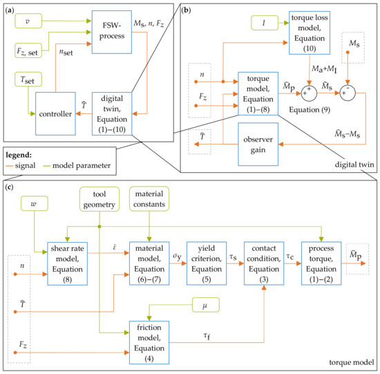
Figure 1.
(a) Complete control structure with (b) the digital twin and (c) the torque model.
The first submodel (Figure 1b) shows the inner structure of the digital twin. The essential element is the block torque model, in which a forward calculation of the estimated process torque is conducted. Subsequently, the process torque is corrected by the torque losses resulting from friction inside the spindle motor and by the acceleration , yielding the calculated spindle torque . The error between the measured and the calculated spindle torque - is the input of the observer gain. The observer gain, similar to a controller, minimizes this error by adjusting an input signal (in this case the calculated temperature ) of the torque model. The calculated welding temperature equals the measured welding temperature T, if produces a zero-approaching torque model error -.
The second submodel (Figure 1c) displays the composition of the torque model. Section 2.1 describes the respective models, as well as their development and interrelation from bottom up.
2.1. Torque Model
The welding temperature and the torque mutually interact: An increase of the applied torque leads to a rise in friction and hence the welding temperature. This leads to thermal softening of the material, which in turn reduces the torque [25]. The process torque was calculated through a series of submodels (Figure 1c). The following assumptions and restrictions (Asm.) were made to derive the submodels:
- The shoulder is cylindrical and the probe is conical. The thread and the three flats on the probe, as well as the concave cavity on the front side of the shoulder, can be neglected [26].
- The tilt angle of the tool α can be neglected.
- The temperature is constant in the shear zone and corresponds to the measured probe temperature.
- The volume and thickness w of the shear zone are constant. The velocity distribution across the shear zone is linear [26].
- Friction and plastic deformation are considered by , which is constant at the entire tool-workpiece interface [26].
- The contact condition is based on Shaw’s friction law [27].
- The von Mises yield criterion can be applied [26,28].
- Coulomb’s friction law can be applied. The friction coefficient μ is constant for the entire tool-workpiece interface [6].
- The yield stress of the workpiece material depends only on the temperature T, the strain ε and the strain rate [29].
According to Roth et al. [26] and Arora et al. [30], the process torque is the cause of the temperature dependent contact shear stress acting on the FSW tool. It can be formulated as:
with the infinitesimal surface element , which lies in radial distance to the center line of the tool. Combining Asm. 1 and the solution of the surface integral in Equation (1) for the tool-workpiece interface yields the formula for the process torque:
where and correspond to the radius of the shoulder and the probe tip, respectively. is the angle of the conically shaped probe and is its length. A sketch of the tool is shown in Figure 2.
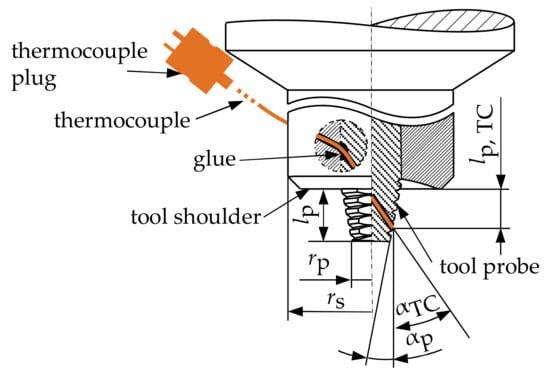
Figure 2.
Sketch of the welding tool, data from [6].
The contact shear stress is the result of the friction and plastic deformation of the material. The relationship between those variables depends on the contact state, which can be differentiated into pure sliding, full sticking and partial sliding/sticking [28]. However, it is generally accepted that both sliding and sticking occur during FSW and that this contact condition is also non-uniform. Several approaches [27,28,31] have been suggested to link the contact shear stress to the shear flow stress and the frictional shear stress . Using the friction law for deformation processes according to Shaw [27] and Doege and Behrens [31] (see Asm. 5 and 6) yields the contact condition, which connects the contact states sliding and sticking in one formula:
Here, j is a natural number describing the transition between Coulomb’s law (for pure sliding) and the friction factor model (for full sticking). j = 2 resulted in a sufficient accuracy of the process torque in an offline simulation. The frictional shear stress can be obtained by applying Asm. 8, resulting in the friction model [26]:
with the friction coefficient μ, whose value is given in Table A1, the axial downward force , and the radius of the shoulder . The shear flow stress can be calculated from the yield stress according to the von Mises yield criterion (Asm. 7):
For the determination of the yield stress , several material models have been discussed in the literature [26,28]. In a preceding offline simulation, the Johnson-Cook yield stress model demonstrated superior performance compared to the Sheppard-Wright model. The Johnson-Cook material model can be described by [32]:
where ε and refer to the strain and the strain rate, respectively. The coefficients , , , and are material constants determined for a specific references strain rate and given in Table A1. T is the temperature in the shear zone, is the melting temperature of the material and is the room temperature. As corresponds to the yield stress of the material at room temperature [33], it is used to determine the strain ε according to Hook’s law:
The Young’s modulus E is given in Table A1. As suggested by Roth et al. [26] and Schmidt [28], the mean shear rate in z direction can be calculated from the RPM-rate n, the width w of the shear zone (see Table A1) as well as the radii and (shear rate model):
By combining the Equations (1)–(8), the process torque was calculated as a function of the calculated temperature , the RPM-rate n, and the axial downward force . The relationship between the individual equations is presented in Figure 1c.
2.2. Digital Twin
The digital twin reverses the relationship, described by the Equations (1)–(8) in order to calculate the welding temperature (see Figure 1). For this purpose, a reduced-order state observer approach was employed, in which the calculated spindle torque was compared to the measured spindle torque . The temperature was the output of the dynamic observer gain and results therefore from the torque model error. To calculate the spindle torque , torque losses inside the motor have to be considered yielding the spindle torque model [18]:
The idling torque results from friction, e.g., in the bearings of the spindle motor, and was measured for different RPM-rates (see Table A2). Intermediate values were determined through linear interpolation. The acceleration torque depends on the moment of inertia I and the time-dependent change of the RPM-rate n:
A value of 0.02285 kg⋅m² was obtained for the moment of inertia I in preliminary experiments. The signal of the welding temperature was determined by closing the observer loop. Thereby, the spindle torque error is minimized by adjusting the calculated temperature input of the torque model. The observer system ensured that the calculated welding temperature converges to the actual welding temperature, assuming that the torque model is sufficiently accurate. For steady-state accuracy, a PI-element was employed. A derivative term was not added due to the measurement noise in the torque model error signal. The values of the observer parameters were tuned with the Matlab PID Tuner. A trade-off between fast convergence and minimal oscillations was achieved for a proportional gain of 0.15 K/(Nm) and an integral gain of 1000 K/(Nm⋅s). The signal of the output was limited by the melting temperature (see Table A1), because the welding temperatures for FSW usually do not exceed this limitation.
2.3. Controller Design
Lastly, a controller was added to the system (Figure 1). An 1 adaptive controller was chosen due to its robustness and decoupled adaptiveness. The controller and its parameters were adopted from Bachmann et al. [18], whereby two adjustments were made: In contrast to Bachmann et al. [18], the calculated temperature and not the measured temperature T was controlled by setting the RPM-rate . As the signal of the calculated temperature compared to the signal of the measured temperature T exhibited extensive noise, the cut-off frequency was reduced from 2π rad/s (approximately 6.28 rad/s), as proposed by Bachmann et al. [17], to 3 rad/s. The filter, however, still passed the typically slow temperature changes for FSW, which lie far below 0.3 rad/s [18].
3. Experimental Validation
The subsystems were validated separately by welding experiments using the set-up depicted in Figure 3. After sufficient performance by the subsystem had been demonstrated, the complete control structure as shown in Figure 1a was tested. All experiments were conducted using an industrial robot (KR 500-2 MT, KUKA AG, Augsburg, Germany), equipped with an FSW spindle and a load cell for an internal control of the axial force during the welding process.
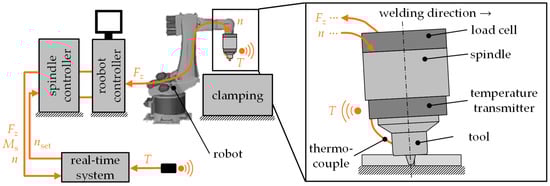
Figure 3.
Experimental set-up based on [6]; a close-up photograph of the tool and the temperature transmitter is given in Figure A1 in the Appendix C.
A real-time system (MicroLabBox, dSPACE GmbH, Paderborn, Germany) and a host PC were added to implement the models and monitor the welding processes. The spindle torque was calculated from the power consumption of the spindle motor by the internal spindle controller. The RPM-rate n and the axial downward force were acquired from the spindle controller and the robot controller, respectively. Those three signals were provided to the real-time system, which was used to implement the models and set the RPM-rate .
3.1. Validation of the Digital Twin
For the validation of the digital twin, the calculated welding temperature was compared to a measured probe temperature T. For this purpose, the probe of the FSW tool was equipped with a volumetric thermocouple of type K with a probe diameter of 0.5 mm. A sheathed thermocouple was used, in order to reduce measurement disturbances from oxidation. [34]. The thermocouple was placed in a drill hole with a diameter of 0.6 mm, at an angle of 30° and a distance to the shoulder of 1.8 mm. It was kept in place by a ceramic glue (Figure 2 and Figure 3). The temperature measuring device designed by Costanzi et al. [35] was used to obtain the temperature signal. The signal was transmitted to the real-time system via wireless local area network (WLAN). The signal from the temperature measurement tool was only employed for performance evaluation and not for temperature control.
To validate the digital twin, ten welding experiments were conducted using an FSW tool with a probe tip radius = 2.35 mm, a length = 6 mm, an angle = 11°, and a shoulder radius = 10 mm. Bead-on-plate welds were made on 8 mm thick plates of EN AW-6082-T6 and EN AW-5083-H111. The tilt angle = 2.5° was constant throughout the experiments. Table 1 shows the process parameters selected for the validation experiments. The set RPM-rate was manually changed during the welding process to test a variation of , which could be caused by the controller in the second phase of the validation. The size of the step Δ differed depending on the welding speed v. In order to prevent tool failure, the was set to 1000 min−1 during the plunge phase for experiments with low RPM-rates (exp. no. 1–3, 5–6 and 9–10). After the plunge phase, the RPM-rate was set to the nominal value according to Table 1. The signal of the temperature was calculated and compared in-line to the signal of the measured temperature T. The experiments were conducted while the internal force controller was activated. Preliminary studies revealed that axial forces of 8.3 kN and 7.8 kN result in defect-free welds and a smooth seam surface for the chosen parameters of the welding speeds, RPM-rates, and FSW tool. In a later analysis, experiment no. 1 was repeated, but with a lower axial downward force (exp. no. 9 and no. 10).

Table 1.
Welding parameters of the step response experiments for the validation of the digital twin; the work piece geometry is shown in Figure A2a in the Appendix C.
Figure 4 presents the validation results of the digital twin for two experiments with a welding speed v of 200 mm/min for the aluminum alloys EN AW-6082-T6 (exp. no. 2) and EN AW-5083-H111 (exp. no. 6), respectively. The temperature measurements show the time-dependent evolution of the welding temperature along the joint. As expected, the temperatures increased with a rising set RPM-rate . The steps in the temperature signals were caused by the incremental increase of the set RPM-rate Δ and are marked by dashed vertical lines. The signals of the temperatures T and all exhibited a time delay to a change of the RPM-rate Δ below one tenth of a second (Figure A4), which was attributed to the reaction time of the spindle controller. For the step response experiments, the steady-state temperature was generally reached after several seconds (Figure A4). For experiments with a high welding speed, e.g., exp. no. 3, 4, 7, and 8, a distinct temperature drop in T was observed. This was attributed to the change in heat transportation phenomena at the start of the welding motion. Additionally, the experimental data in Figure 4a,b exhibited oscillations in the signals. This was attributed to the low stiffness of the industrial robot and unintentional excitation with the eigenfrequency at ∊ [800, 900]. Due to the general latency of heat transfer, the oscillations in the signal of the measured temperature T were significantly weaker than in that of the calculated temperature . This can primarily be attributed to the higher measuring dynamics of the spindle controller compared to the temperature measuring tool. Additionally, the calculation of from the oscillating signals (, , and ) resulted in an amplification of the oscillations in the signal of the calculated temperature .
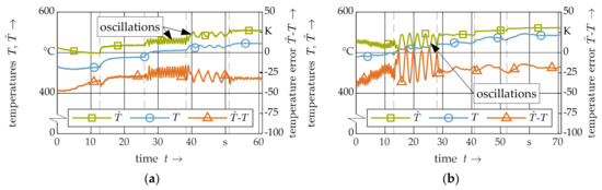
Figure 4.
Validation of the digital twin: comparison of the measured temperature T (blue circle) and calculated temperature (green square) with the temperature model error -T (orange triangle) for (a) exp. no. 2 (an enlarged cutout is shown in Figure A4) and (b) exp. no. 6; the corresponding welding parameters are given in Table 1.
The performance of the digital twin was quantified using the root mean squared percentage error (RMSPE, see Equation (A1)) between the measured and the calculated temperature (orange curve with triangles in Figure 4). The experiments no. 2 and no. 6 exhibited an average performance with an RMSPE of 6.55% and 6.04%, respectively. The error RMSPE was below 8% for all experiments. The absolute temperature error -T was approximately constant in most experiments. In total, the absolute mean temperature errors for all experiments ranged from −31 K (exp. no. 3) to +15 K (exp. no. 1). In experiment no. 1, positive temperature errors -T occurred. By repeating the same experiment, but with lower axial downward forces (see Table 1, exp. no. 9–10), it was observed that with a decrease of the force, the temperature error -T also partially changed to a negative value and ranged from +15 K (exp. no. 1) over −17 K (exp. no. 9) to +5 K (exp. no. 10). This leads to the conclusion that the relationship between the axial downward force and the welding temperature was not accurately modelled. A comparison between the temperature errors -T for experiments with different welding speed v also revealed that the error -T generally increased with the welding speed v. For equal set RPM-rates , the absolute measured spindle torque || increased with the welding speed v in all experiments. This indicates an indirect influence of the welding speed v on the measured spindle torque and therefore on the calculated temperature . The welding speed v was, however, otherwise neglected in the torque model. In summary, the varying temperature errors -T reveal a potential for improving the torque model.
3.2. Validation of the Complete Control Structure
For the evaluation of the complete system, three bead-on-plate welds, including one with a geometry which deliberately caused heat accumulation, and one lap weld were made with the aluminum alloy EN AW-6082-T6 (see Table 2). The validation experiments for the digital twin revealed significant temperature errors for some process parameter combinations. For these experiments, insufficient control performance was expected due to an inaccurate calculated temperature . Consequently, a parameter setting (see Table 2), which in previous experiments produced only a small temperature error of +8.5 K, was selected for the first validation experiment. To prevent expected vibrations of the robot, a lower set welding temperature of 500 °C was chosen. A second bead-on-plate weld was made for a parameter setting that produced a higher temperature error of approximately −31 K in an earlier experiment. As it was believed that the temperature errors were reproducible and could result in an insufficient control performance, a process parameter dependent correction offset was added to the signal of the calculated temperature . The value of the offset equaled the average temperature error, obtained from experiment no. 3. This enabled the validation of the complete control structure, even with the inaccurate temperature calculation. Finally, butt joints were made on a narrow geometry described in Bachmann et al. [7], which deliberately caused heat accumulation. For comparison, a second part with the same geometry was welded with a constant set RPM-rate (without temperature control).
Table 2.
Welding parameters of the experiments for the validation of the complete control structure; the work piece geometries are shown in Figure A2 (exp. no. 11–13) and Figure A3 (exp. no. 14) in the Appendix C.
Figure 5 shows the results from the validation of the complete control structure for two bead-on-plate welds without (a) and with (b) the application of a correction offset . The dashed vertical lines mark the time in seconds when the controller was activated.

Figure 5.
Validation of the complete control structure: Comparison of the measured temperature T (blue circle) to the calculated temperature (green square) as well as the temperature model error -T (orange triangle) and the set RPM-rate (black asterisk) for two bead-on-plate welds, exp. no. 11 without (a) and exp. no. 12 with (b) the application of a correction offset ; the corresponding welding parameters are given in Table 2.
As shown in Figure 5a, the reaction of the controller resulted in an approach of the calculated temperature (green squares) to the set welding temperature (dashed horizontal line). The small temperature error was expected and resulted in a small control deviation for the measured temperature T (<10 K). With the activation of the controller after approximately 3 s, the set RPM-rate (black asterisk) dropped from 1000 min−1 to approximately 670 min−1. At the beginning, the controller experienced a small undershoot, which was brief enough to not influence the signal of the measured temperature T. This undershoot was more pronounced in experiment no. 12 (Figure 5b) and was already described in [6]. It is caused by the temperature prediction with the PT1-element of the 1 adaptive controller. The impact of the undershoot was limited by setting the RPM-rate saturation value to 400 min−1.
With the application of the correction offset , (Figure 5b), the signal of the calculated temperature was successfully held constant at a value of 31 K (=) above 530 °C. The deviation of the measured temperature T from the commanded temperature was, however, approximately 20 K. The temperature error −T in experiment no. 12 was smaller (−10 K) than in the previous welding experiment no. 3 (−31 K), even though both experiments were conducted with the same process parameters. The inadequate value of the correction offset led to an overreaction of the controller and a relatively high set RPM-rate = 1350 min−1 (black asterisk).
The lap weld from experiment no. 13 in Figure 6a produced results similar to the bead-on-plate weld of the experiment no. 11. The signal of the calculated temperature was also successfully held constant at a value of 30 K (=) above 530 °C. An unexpected positive temperature error, together with the negative correction offset , resulted in a control deviation for the measured temperature T of approximately 45 K, which was deemed too high. No undershoot in the signal of the set RPM-rate occurred.
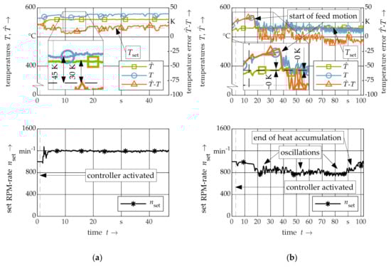
Figure 6.
Validation of the complete control structure: comparison of the measured temperature T (blue circle) to the calculated temperature (green square) as well as the temperature model error -T (orange triangle) and the set RPM-rate (black asterisk) for a lap weld with the application of the correction offset i.e. experiment no. 13 (a) and a bead-on-plate weld without a correction offset , i.e. experiment no. 14 (b); the corresponding welding parameters are given in Table 2.
The last experiment was again conducted without a correction offset . Here, heat accumulation was intentionally created by selecting a workpiece with a small width, as described by [7] (40 mm, see Figure A3 in the Appendix C). Figure 6b shows the temperature dropping effect of the start of the welding motion after 18 s. Even without a correction offset , the temperature error was low during the welding phase. Due to a set RPM-rate in the range of 800–900 min−1, vibrations of the industrial robot occurred. The oscillations were transmitted to the measurement signals, which were used to calculate the temperature . The resulting oscillating set RPM-rate further amplified this behavior. It is believed that a re-adjustment of the second order Butterworth filter of the 1 adaptive controller could break this self-reinforcing interaction, however at the cost of the control dynamics. Apart from these oscillations, the controller held the calculated temperature at the set temperature of 530 °C. At around 89 s, the tool left the narrow strip of the workpiece. From there on, no particular heat accumulation occurred. The control system reacted to this by increasing the set RPM-rate . Due to the low temperature error, the controller deviation of the measured temperature T approached zero for the entire welding phase.
Figure 7a shows a photograph of the resulting weld from experiment no. 14. For comparison, a weld made without temperature control is depicted in Figure 7b. The comparison illustrates that the controller prevented heat accumulation and ensured a high weld quality because the weld, which was fabricated with a constant set RPM-rate, exhibited excessive flash, while with the control, no flash occurred at all. Figure 7a also shows the impact of the afore-mentioned vibrations. The weld surface features wide grooves that resulted from the visible displacement of the industrial robot and the tool during welding.
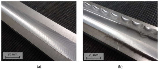
Figure 7.
Welds with the parameter setting from experiment no. 14 with (a) and without (b) temperature control.
4. Discussion
A state feedback control of the welding temperature, using a digital twin, is feasible. The correlation of the temperature error with the process parameters revealed that the influence of the welding speed v and the axial downward force on the calculated temperature should be further examined in the future. Given that the temperature error remained approximately constant while varying the set RPM-rate , it was concluded that the relation between and the welding temperature T was modelled successfully.
Some experiments with low RPM-rates (exp. no. 1–3, 5, and 6) featured higher temperature errors at the beginning of the weld. These experiments were conducted with an initial set RPM-rate = 1000 min−1 during the plunging phase, in order to avoid tool breakage. This resulted in a severe drop of , e.g., from 1000 min−1 to 600 min−1 (exp. no. 2), which required a waiting time of 10 to 15 s until the welding temperature recovered and the steady-state temperature for this set RPM-rate was approached. In these cases, the digital twin only produced sufficiently accurate results after this waiting time.
A process parameter dependent correction offset was applied in the experiments no. 12 and no. 13 to validate the complete control structure for parameter sets with temperature errors above 10 K. It was shown that the application of a process parameter dependent and constant correction offset generally did not improve the control performance as different thermal behaviors in the welding experiments led to an inadequate choice for the value of the correction offset . These deviations could have been caused by disturbances, like tool abrasion and varying positions of the thermocouples in the tool. The repetition of the experiments with a new tool could lead to lower temperature errors. Another cause for the varying temperature errors could have been the assumptions 1–9, which were made in order to derive a torque model that can be calculated in real time. These assumptions include the negligence of the tilt angle of the tool α and of the threads on the probe which are both temperature-influencing parameters. Minor temperature errors could also stem from imprecise temperature measurements, as thermocouples degrade over time. This could explain errors of up to 4.65 K, according to the IEC 60584-1:2013 [36].
5. Conclusions
In this paper, a state feedback temperature control by means of a digital twin is introduced. The digital twin served as a soft sensor to control the welding temperature. It is based on a temperature dependent analytical torque model, which uses measurements of the RPM-rate n and the axial downward force to calculate the process torque . The deviation between the calculated and the measured torque was minimized to obtain the temperature signal . The temperature was then held at the desired value by an 1 adaptive controller. Both the digital twin and the control system were validated through several welding experiments with different process parameters. The following conclusion were drawn from the validation:
- The model errors of the welding temperature range from −31 K to +15 K and primarily depend on the welding speed v and the axial downward force . It is believed that the model performance can be improved by finding suitable submodels to account for the welding speed v and the axial downward force .
- The controller was able to correctly adjust the set RPM-rate , so that the calculated temperature was held constant at the desired value.
- The low stiffness of the FSW machine (industrial robot) posed challenges, as vibrations were amplified through the digital twin and resulted in significant oscillations in the signals.
- The application of a temperature error correction offset cannot be recommended. The controller deviation was smaller than 10 K for all experiments without the correction offset, including an experiment with a workpiece that deliberately caused heat accumulation.
- The digital twin is only valid for the weld phase of the FSW process. The preceding and consecutive phases, during which the tool plunges into and retracts from the workpiece, were not modelled. This makes the digital twin most likely not applicable for these two phases.
Author Contributions
Conceptualization, A.B.; methodology, A.B. and M.E.S.; software, M.E.S. and T.M.; validation, M.E.S. and T.M.; formal analysis, A.B.; investigation, M.E.S.; resources, A.B. and M.E.S.; data curation, M.E.S.; writing—original draft preparation, M.E.S.; writing—review and editing, A.B. and M.F.Z.; visualization, M.E.S.; supervision, M.F.Z.; project administration, A.B. and M.E.S.; funding acquisition, M.F.Z. M.E.S. and A.B. contributed equally to this paper. All authors have read and agreed to the published version of the manuscript.
Funding
The IGF-research project no. 19.516 N of the Research Association on Welding and Allied Processes of the DVS has been funded by the AiF within the framework for the promotion of industrial community research (IGF) of the Federal Ministry for Economic Affairs and Energy because of a decision by the German Bundestag.
Acknowledgments
We thank Catarina Piffer for helping to compare different submodels for the digital twin.
Conflicts of Interest
The authors declare no conflict of interest.
Appendix A
Table A1.
Numerical values of the torque model parameters with units and the corresponding literature sources.
Table A1.
Numerical values of the torque model parameters with units and the corresponding literature sources.
| Parameter | EN AW-5083-H111 | EN AW-6082-T6 | Unit | ||
|---|---|---|---|---|---|
| Values | Reference | Values | Reference | ||
| μ | 0.4 | [26] | 0.4 | [26] | – |
| j | 2 | – | 2 | – | – |
| A | 143 | [37] | 285 | [38] | N/mm2 |
| B | 554 | [37] | 94 | [38] | N/mm2 |
| C | 0.001 | [37] | 0.002 | [38] | – |
| m | 0.895 | [37] | 1.34 | [38] | – |
| k | 0.526 | [37] | 0.41 | [38] | – |
| 1 | [37] | 1 | [38] | – | |
| 25 | – | 25 | – | °C | |
| 620 | [37] | 588 | [38] | °C | |
| w | 1.2 | [6] | 1.2 | [6] | mm |
| E | 70 000 | [39] | 70 000 | [39] | N/mm2 |
Table A2.
Idling torque depending on the set RPM-rate .
Table A2.
Idling torque depending on the set RPM-rate .
| in min−1 | in Nm | in min−1 | in Nm | in min−1 | in Nm |
|---|---|---|---|---|---|
| 100 | 1.4278 | 1300 | 2.2496 | 2600 | 2.5914 |
| 200 | 1.3145 | 1400 | 2.2703 | 2700 | 2.8822 |
| 300 | 1.3475 | 1500 | 2.2905 | 2800 | 3.1876 |
| 400 | 1.3948 | 1600 | 2.2788 | 2900 | 3.4932 |
| 500 | 1.4701 | 1700 | 2.2490 | 3000 | 3.8079 |
| 600 | 1.6040 | 1800 | 2.2191 | 3100 | 4.2209 |
| 700 | 1.7380 | 1900 | 2.1893 | 3200 | 4.6394 |
| 800 | 1.8544 | 2000 | 2.1603 | 3300 | 5.0105 |
| 900 | 1.9620 | 2200 | 2.2487 | 3400 | 5.3163 |
| 1000 | 2.0696 | 2300 | 2.3296 | 3500 | 5.6205 |
| 1100 | 2.1775 | 2400 | 2.4098 | 3600 | 5.6981 |
| 1200 | 2.2284 | 2500 | 2.4902 | – | – |
Appendix B
The Root Mean Square Percentage Error (RMSPE) of the calculated temperature was calculated using the following equation:
with the data size q, the index of summation i, and the measured temperature T.
Appendix C

Figure A1.
Close-up photograph of the tool with the thermocouple and the temperature transmitter.

Figure A2.
(a) Geometry for experiments no. 1–12 and (b). Experiment no. 13. The welds are indicated in grey.

Figure A3.
Geometry for experiment no. 14, data from [7], the narrowed zone causes heat accumulation. The welds are indicated in grey.

Figure A4.
Enlarged cutout of Figure 4a (exp. no. 2) showing the dynamic behavior of the measured temperature T (blue circle) and the calculated temperature (green square) for a stepwise increase of the RPM-rate
References
- Grätzel, M.; Schick-Witte, K.; Köhler, T.; Bergmann, J.P.; Weigl, M. Rührreibschweißmethoden für Anwendungen in der Elektromobilität: Eine vergleichende Gegenüberstellung auf Basis prozesstechnologischer und mechanischer Eigenschaften: (‘Friction Stir Welding for Application in the Electric Mobility Sector: A Comparision Regarding Technological and Mechanical Properties’). DVS Ber. 2019, 355, 554–559. [Google Scholar]
- MT Aerospace AG. MT Aerospace ships the first tank for Ariane 6 to ArianeGroup in Bremen. Available online: https://www.mt-aerospace.de/news-details-en/mt-aerospace-ships-the-first-tank-for-ariane-6-to-arianegroup-in-bremen.html (accessed on 12 May 2020).
- Masny, H.; Heinrich, G.; Kahnert, M.; Knerr, D. Rührreibschweißen in der Fertigung von Tanks bei der neuen Trägerrakete Ariane 6: (Friction Stir Welding for the Manufacturing of Tanks for the New Carrier Rocket Ariane 6). DVS Ber. 2019, 355, 134–138. [Google Scholar]
- Bachmann, A.; Krutzlinger, M.; Zaeh, M.F. Influence of the welding temperature and the welding speed on the mechanical properties of friction stir welds in EN AW-2219-T87. IOP Conf. Ser. Mater. Sci. Eng. 2018, 373. [Google Scholar] [CrossRef]
- Suenger, S.; Kreissle, M.; Kahnert, M.; Zaeh, M.F. Influence of Process Temperature on Hardness of Friction Stir Welded High Strength Aluminum Alloys for Aerospace Applications. Procedia CIRP 2014, 24, 120–124. [Google Scholar] [CrossRef]
- Bachmann, A.; Gamper, J.; Krutzlinger, M.; Zens, A.; Zaeh, M.F. Adaptive model-based temperature control in friction stir welding. Int. J. Adv. Manuf. Technol. 2017, 93, 1157–1171. [Google Scholar] [CrossRef]
- Bachmann, A.; Zaeh, M.F. Pyrometer-Assisted Temperature Control in Friction Stir Welding. In Proceedings of the 11th International Friction Stir Welding Symposium, Québec, QC, Canada, 17–20 May 2016. [Google Scholar]
- De Backer, J.; Bolmsjö, G.; Christiansson, A.-K. Temperature control of robotic friction stir welding using the thermoelectric effect. Int. J. Adv. Manuf. Technol. 2014, 70, 375–383. [Google Scholar] [CrossRef]
- Cederqvist, L.; Garpinger, O.; Hägglund, T.; Robertsson, A. Cascade control of the friction stir welding process to seal canisters for spent nuclear fuel. Control Eng. Pract. 2012, 20, 35–48. [Google Scholar] [CrossRef]
- Fehrenbacher, A.; Cole, E.G.; Zinn, M.R.; Ferrier, N.J.; Duffie, N.A.; Pfefferkorn, F.E. Towards Process Control of Friction Stir Welding for Different Aluminum Alloys. In Friction Stir Welding and Processing VI; Mishra, R.S., Ed.; Wiley: Hoboken, NJ, USA, 2011; pp. 381–388. ISBN 9781118002018. [Google Scholar]
- Fehrenbacher, A.; Duffie, N.A.; Ferrier, N.J.; Pfefferkorn, F.E.; Zinn, M.R. Toward Automation of Friction Stir Welding Through Temperature Measurement and Closed-Loop Control. J. Manuf. Sci. Eng. 2011, 133, 1. [Google Scholar] [CrossRef]
- Fehrenbacher, A.; Duffie, N.A.; Ferrier, N.J.; Pfefferkorn, F.E.; Zinn, M.R. Effects of tool-workpiece interface temperature on weld quality and quality improvements through temperature control in friction stir welding. Int. J. Adv. Manuf. Technol. 2014, 71, 165–179. [Google Scholar] [CrossRef]
- Fehrenbacher, A.; Duffie, N.A.; Ferrier, N.J.; Zinn, M.R.; Pfefferkorn, F.E. Temperature measurement and closed-loop control in friction stir welding. In Proceedings of the 8th International Friction Stir Welding Symposium, Timmendorfer Strand, Germany, 18–20 May 2010. [Google Scholar]
- Fehrenbacher, A.; Pfefferkorn, F.E.; Zinn, M.R.; Ferrier, N.J.; Duffie, N.A. Closed-loop control of temperature in friction stir welding. In Proceedings of the 7th International Friction Stir Welding Symposium, Awaji Island, Japan, 20–22 May 2008. [Google Scholar]
- Fehrenbacher, A.; Smith, C.B.; Duffie, N.A.; Ferrier, N.J.; Pfefferkorn, F.E.; Zinn, M.R. Combined Temperature and Force Control for Robotic Friction Stir Welding. J. Manuf. Sci. Eng. 2014, 136, 1. [Google Scholar] [CrossRef]
- Ross, K.; Sorensen, C. Advances in Temperature Control for FSP. In Friction Stir Welding and Processing VII; Mishra, R., Mahoney, M.W., Sato, Y., Hovanski, Y., Verma, R., Eds.; Springer International Publishing: Cham, Switzerland, 2016; pp. 301–310. ISBN 978-3-319-48582-9. [Google Scholar]
- Ross, K.; Sorensen, C. Paradigm Shift in Control of the Spindle Axis. In Friction Stir Welding and Processing VII; Mishra, R., Mahoney, M.W., Sato, Y., Hovanski, Y., Verma, R., Eds.; Springer International Publishing: Cham, Switzerland, 2016; pp. 321–328. ISBN 978-3-319-48582-9. [Google Scholar]
- Bachmann, A.; Roehler, M.; Pieczona, S.J.; Kessler, M.; Zaeh, M.F. Torque-based adaptive temperature control in friction stir welding: A feasibility study. Prod. Eng. Res. Devel. 2018, 12, 391–403. [Google Scholar] [CrossRef]
- Krutzlinger, M.; Marstatt, R.; Costanzi, G.; Bachmann, A.; Haider, F.; Zaeh, M.F. Temperature Control for Friction Stir Welding of Dissimilar Metal Joints and Influence on the Joint Properties. KEM 2018, 767, 360–368. [Google Scholar] [CrossRef]
- Ross, K.; Sorensen, C. Investigation of Methods to Control Friction Stir Weld Power with Spindle Speed Changes. In Friction Stir Welding and Processing VI; Mishra, R.S., Ed.; Wiley: Hoboken, NJ, USA, 2011; pp. 345–352. ISBN 9781118002018. [Google Scholar]
- Magalhães, A. Thermo-Electric Temperature Measurements in Friction Stir Welding—Towards Feedback Control of Temperature; University West: Trollhättan, Sweden, 2016; ISBN 978-91-87531-42-2. [Google Scholar]
- Augustin, S.; Fröhlich, T.; Krapf, G.; Bergmann, J.-P.; Grätzel, M.; Gerken, J.A.; Schmidt, K. Herausforderungen der Temperaturmessung während des Rührreibschweißprozesses: (Challenges of temperature measurement during the friction stir welding process). Tech. Mess. 2019, 86, 765–772. [Google Scholar] [CrossRef]
- Lahiri, S.K. Multivariable Predictive Control. Applications in Industry, 1st ed.; John Wiley & Sons Ltd: Hoboken, NJ, USA, 2017; ISBN 9781119243595. [Google Scholar]
- Bortoff, S.A.; Laughman, C.R. An Extended Luenberger Observer for HVAC Application using FMI. In Proceedings of the 13th International Modelica Conference, Regensburg, Germany, 4–6 March 2019. [Google Scholar]
- Colligan, K.J.; Mishra, R.S. A conceptual model for the process variables related to heat generation in friction stir welding of aluminum. Scr. Mater. 2008, 58, 327–331. [Google Scholar] [CrossRef]
- Roth, A.; Hake, T.; Zaeh, M.F. An Analytical Approach of Modelling Friction Stir Welding. Procedia CIRP 2014, 18, 197–202. [Google Scholar] [CrossRef]
- Shaw, M.C. The role of friction in deformation processing. Wear 1963, 6, 140–158. [Google Scholar] [CrossRef]
- Schmidt, H.N.B. Modelling thermal properties in friction stir welding. In Friction Stir Welding: From Basics to Applications; Lohwasser, D., Ed.; Woodhead Publishing: Cambridge, UK; CRC Press: Boca Raton, FL, USA, 2010; pp. 277–313. ISBN 9781845694500. [Google Scholar]
- Roth, A. Modellierung des Rührreibschweißens unter besonderer Berücksichtigung der Spalttoleranz: (Modelling of friction stir welding under special consideration of the gap tolerance). Ph.D. Thesis, Technical University of Munich, Munich, Germany, 2016. [Google Scholar]
- Arora, A.; Nandan, R.; Reynolds, A.P.; DebRoy, T. Torque, power requirement and stir zone geometry in friction stir welding through modeling and experiments. Scr. Mater. 2009, 60, 13–16. [Google Scholar] [CrossRef]
- Doege, E.; Behrens, B.-A. Handbuch Umformtechnik. Grundlagen, Technologien, Maschinen. (Forming Technology Handbook: Basics, Technologies, Machines); Springer: Berlin, Germany, 2010; ISBN 3642042481. [Google Scholar]
- Johnson, G.R.; Cook, W.H. Fracture characteristics of three metals subjected to various strains, strain rates, temperatures and pressures. Eng. Fract. Mech. 1985, 21, 31–48. [Google Scholar] [CrossRef]
- Kuykendall, K. An Evaluation of Constitutive Laws and their Ability to Predict Flow Stress over Large Variations in Temperature, Strain, and Strain Rate Characteristic of Friction Stir Welding. Ph.D. Thesis, Brigham Young University, Provo, UT, USA, 2014. [Google Scholar]
- RS Components GmbH. IEC Mineral Insulated Thermocouple with Miniature Thermocouple Plug Type K (Grounded Junction): Fast response Type ‘K’ Thermocouple, 0.5 mm diameter with grounded hot junction. Datasheet. Available online: https://docs.rs-online.com/6861/0900766b815bb3bd.pdf (accessed on 24 June 2020).
- Costanzi, G.; Bachmann, A.; Zäh, M.F. Entwicklung eines FSW-Spezialwerkzeugs zur Messung der Schweißtemperatur: (Development of an FSW tool to measure the Welding Temperature). DVS Ber. 2017, 337, 119–125. [Google Scholar]
- International Electrotechnical Commission. Thermocouples—Part 1: EMF Specifications and Tolerances; IEC 60584-1:2013; VDE Verlag: Berlin, Germany, 2013. [Google Scholar]
- Clausen, A.H.; Børvik, T.; Hopperstad, O.S.; Benallal, A. Flow and fracture characteristics of aluminium alloy AA5083-H116 as function of strain rate, temperature and triaxiality. Mater. Sci. Eng. A 2004, 364, 260–272. [Google Scholar] [CrossRef]
- Birsan, D.; Scutelnicu, E.; Visan, D. Behaviour Simulation of Aluminium Alloy 6082-T6 during Friction Stir Welding and Tungsten Inert Gas Welding. Recent Adv. Manuf. Eng. 2011, 30, 103–108. [Google Scholar]
- Lundberg, S. Design Philosophy. TALAT Lecture 2204. 1994. Available online: https://www.slideshare.net/corematerials/talat-lecture-2204-design-philosophy (accessed on 30 May 2020).
© 2020 by the authors. Licensee MDPI, Basel, Switzerland. This article is an open access article distributed under the terms and conditions of the Creative Commons Attribution (CC BY) license (http://creativecommons.org/licenses/by/4.0/).