Abstract
Common forensic entomology practice has been to collect the largest Diptera larvae from a scene and use published developmental data, with temperature data from the nearest weather station, to estimate larval development time and post-colonization intervals (PCIs). To evaluate the accuracy of PCI estimates among Calliphoridae species and spatially distinct temperature sources, larval communities and ambient air temperature were collected at replicate swine carcasses (N = 6) throughout decomposition. Expected accumulated degree hours (ADH) associated with Cochliomyia macellaria and Phormia regina third instars (presence and length) were calculated using published developmental data sets. Actual ADH ranges were calculated using temperatures recorded from multiple sources at varying distances (0.90 m–7.61 km) from the study carcasses: individual temperature loggers at each carcass, a local weather station, and a regional weather station. Third instars greatly varied in length and abundance. The expected ADH range for each species successfully encompassed the average actual ADH for each temperature source, but overall under-represented the range. For both calliphorid species, weather station data were associated with more accurate PCI estimates than temperature loggers associated with each carcass. These results provide an important step towards improving entomological evidence collection and analysis techniques, and developing forensic error rates.
1. Introduction
Determining time of death is a significant element of solving crimes, yet it is a difficult piece of information to estimate using existing, and often fragmented, evidence collected during a death scene investigation. Patterns of postmortem insect succession and development are common tools used to help narrow the estimated time since death, a time range commonly referred to as the postmortem interval (PMI) [1,2]. Indeed, insects provide valuable clues towards narrowing the estimate of the time since death, however, the term PMI can be misleading as it implies the entire time elapsed since death, and not just the insect activity [3]. Larval dipteran evidence provides information on the length of time those insects have been present on a body postmortem (i.e., how long the resource has been colonized) which, excluding cases of myiasis, does not always correspond to the actual time since death [3,4]. For this reason, forensic entomologists often use the term minimum postmortem interval (PMImin) or the minimum amount of time elapsed since death as indicated by insect development [1]. Death scenes can be highly variable in their circumstances and insect colonization patterns immediately following death cannot always be assumed. For example, the arrival of insects can be delayed if a death occurs indoors [5], if the decedent is wrapped in cloth or like material [6], if the remains are altered by chemicals [7], or if the remains are burned [8]. Therefore, we use the term post-colonization interval (PCI) here when we refer to the time from insect colonization until discovery of the body [3].
The primary insect colonizers of decomposing bodies are blow flies (Diptera: Calliphoridae) [9,10]. The greatest influence on blow fly larval development is temperature, since insects are poikilothermic [1]. Therefore, the amount of time required for calliphorid larvae to develop depends on environmental temperature. In order to standardize development time for temperature dependent development, temperature data are commonly converted to accumulated degree hours (ADH) using thermal summation models [11,12,13]. However, there are many biotic and abiotic factors that can influence larval development, thus making it difficult to accurately estimate the initial time of colonization [14]. For example, rain [15], drugs [16,17,18], predation [19], larval sex [20], geographic location and population genetics [21,22], tissue type [23], and bacteria [24] can all significantly affect larval development by either increasing or decreasing the time required for carrion flies to complete their life cycle.
With all of this potential for variability at death scenes, the Daubert standard [25] and the 2009 National Academy of Sciences Report [26] suggest that laboratory and field variability studies are important to understanding how different factors affect insect development, such as the latter in this paper. Establishing a better understanding of the naturally occurring variability and factors that influence development is necessary to improve evidence collection and analysis techniques that can estimate any indexed concept, such as PCI or PMI, as accurately as possible [3,27]. Investigators at the scene may only collect the largest larval specimens from a body, on the assumption that they are the most developed, and, therefore, could be missing essential information for developing a more concise PMI estimate—even though protocols suggest collecting larvae of variable sizes [1,2,4,28]. Studies have shown that a larval mass can contain multiple blow fly species with abundances that change over time [29]. By only collecting the largest specimens, entire species that are potentially further along in their life cycle (i.e., older) but smaller in size could go unnoticed and uncollected, and thus an inaccurate estimate of the PCI would be generated based solely on the largest but perhaps not oldest larvae. For example, at 25 °C, a 10 mm Cochliomyia macellaria (Fabricius) (Diptera: Calliphoridae) larva would indicate 58 h [30] while a 9 mm Phormia regina (Meigen) (Diptera: Calliphoridae) larva would indicate 66 h [31]. Field studies like this one are important for investigating how different larval sizes (and within an instar) may lead to variable PCI estimates.
Another common practice in forensic entomology is to use the nearest, certified weather station to the death scene and previously published larval development data in order to determine insect developmental time [1,2]. While a weather station is the best source for historically accurate temperature data, it cannot be assumed that the station accurately reflects the microhabitat temperatures of a scene that is not near the said weather station [14,32]. Temperature variation between the death scene and weather station could potentially affect the accuracy of PCI estimates.
The objective of this study was to conduct a field study using multiple vertebrate carcasses to assess variation in PCI estimates derived from different temperature sources and published developmental data for two Calliphoridae species. The goal was not to build predictive models for PMI based on calliphorid life history traits, as has been done in other important studies [33,34,35], but rather, to explore how collecting multiple larval sizes of calliphorid species and using temperature data from multiple sources affected the range of PCIs that were calculated using different data sources. Our overall goal was to explore how multiple sources of variation in larval size and sources of temperature (as discussed by Amendt [4]) affected PCI calculations/estimates in a field study. ADH ranges were derived from temperature data sets acquired from instruments located at varying distances from the carcasses (i.e., individual carcass (0.90 m), microhabitat (0.90 m average of six carcasses), local (1.63 km), regional (7.61 km)), and used to calculate PCI estimates in order to evaluate how temperature sources influence ADH associated PCI estimates. We hypothesized that different Calliphoridae species would colonize the resource at different times resulting in larval size variation on and among carcasses, and that the temperature source nearest the carcasses (microhabitat) would provide temperatures most similar to what the larvae experience. Therefore, we predicted that different species, and larval sizes, would yield different PCI estimates and that the data from the closest temperature source to the carcasses would result in the most accurate PCI estimate. However, we also predicted that PCI estimates, regardless of temperature source utilized, would differ from the actual PCI due to differences in the published laboratory conditions (where developmental data were generated) and the field study conditions.
2. Materials and Methods
2.1. Study Site
The study was conducted from 19–27 August 2014 at Purdue University’s Forensic Entomology Research Compound in West Lafayette, Indiana (40°25′36.0″ N, 86°56′57.0″ W). Six (three male and three female) swine carcasses (Sus scrofa L.), averaging 19.65 kg (± 5.44 SD) and approximately 80.0 cm in length, were used as surrogates for human decomposition [1,36]. Carcasses were purchased from a local swine farm post-euthanization and therefore exempt from university Institutional Animal Care and Use Committee (IACUC) review. Carcasses were immediately placed inside two secured plastic bags during transport to the site (approximately 4 h), as previously described [37,38,39,40]. The carcasses were exposed along two East-West running transects approximately 50 m apart in a grassy field surrounded by deciduous forest. All carcasses were oriented on their left side with heads directed north and placed on top of stainless steel powder-coat painted grates (~1.0 m2, ~5.0 cm2 openings) located on the ground to allow for lifting the individual carcasses during sample collection. Cages (~1.0 m3) constructed of chicken mesh wire and treated lumber were secured over the carcasses and the grates to prevent vertebrate scavenging. Insect communities were sampled every 12 h at approximately 700 h and 1900 h for eight consecutive days (see Larval Collections and Measurements below), which was the amount of time required for the carcasses to fully decompose to only bones and skin, and for the dipteran larvae to enter the post-feeding dispersal stage.
2.2. Temperature
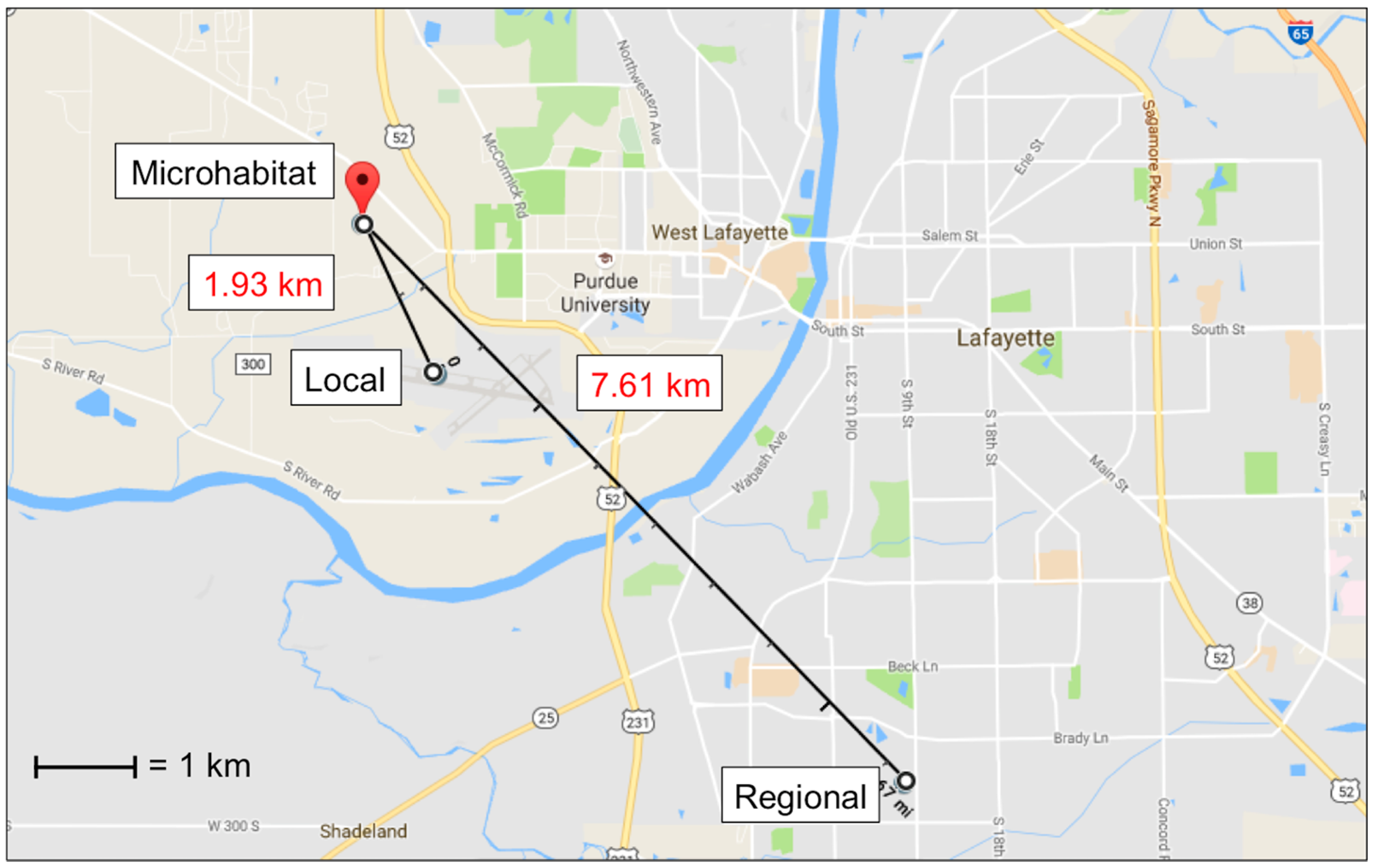
Ambient temperature at each carcass was recorded every 15 min using one HOBOTM temperature logger (Onset Computer Corporation, Bourne, MA, USA) per carcass attached to the east side of each anti-vertebrate scavenging cage approximately 0.90 m off the ground. The individual temperature source refers to the corresponding temperature logger for each carcass at 0.9 m distance. Temperature data from all six loggers were averaged to determine the temperature of the microhabitat source. Local source temperature data were acquired from the Purdue University Airport (40°24’48.5” N, 86°56’26.1” W) weather station, located 1.63 km southeast of the study site. Regional source temperature data were acquired from a Lafayette, Indiana weather station (MAU199) located 7.61 km southeast of the study site (40°22’40” N, 86°53’13” W) (Figure 1). Both local and regional sources recorded temperature at least once every hour throughout the study.
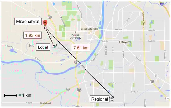
Figure 1.
Map showing the location of and distances between the microhabitat (HOBO temperature loggers), local (Purdue University Airport weather station), and regional (Lafayette weather station) temperature sources. The microhabitat was the average of temperatures measured at each of the six carcasses. (Map: Google, Google).
2.3. Larval Collections and Measurements
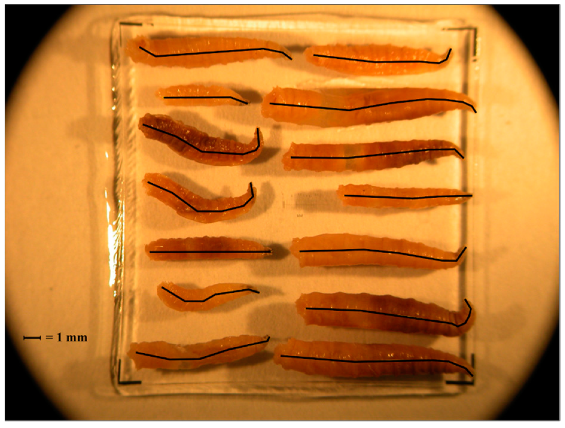
At each sampling period, blow fly larvae were collected using a single cotton-tipped swab (Puritan Medical Products, Guilford, ME, USA) from three different areas of a single larval mass located on the carcass, and stored at −20 °C. Larval instars were determined based on the number of spiracular slits, as discussed elsewhere [41,42]. Third instars were identified to species level using published taxonomic keys for larvae [43,44] and then stored in 100% molecular grade ethanol. Cochliomyia macellaria and P. regina were used for PCI analyses due to specimen abundance and availability of previously published development data [30,31]. Each larva was photographed on a 2 mm micrometer slide and each body length was measured to the nearest 0.01 mm in ImageJ 1.46r [45]. This was done by setting the scale using the micrometer and measuring a line drawn through the larval midline while taking care to follow the curvature of each specimen (Figure 2).

Figure 2.
Example of third instars photographed on a micrometer slide and measured in ImageJ. Black lines indicate the midline that was measured in order to determine length of the larva.
2.4. ADH Ranges and Post-Colonization Intervals
All ADH ranges and PCIs were determined for third instars, since they were the most developed larvae collected and provide the most reliable identification using morphology for Calliphoridae larvae of forensic relevance [46]. Two ADH value sets (min, median, max) for C. macellaria and P. regina were calculated: “expected” ADH ranges using published laboratory-reared larval developmental data sets [30,31] and “actual” ADH ranges using temperatures recorded by the spatially distinct temperature sources (see Temperature section above for more details). Expected ADH ranges are those taken from the published data sets [30,31] that represent the expected ADH necessary for larvae of each species to reach the third instar stage or certain third instar lengths. Actual ADH ranges presumably reflect the temperature conditions of the larvae during decomposition for a given source. Actual ADH values for each species were then compared to expected ADH values. PCI estimates were also derived from the expected ADH ranges calculated for each temperature source and compared to the actual PCIs.
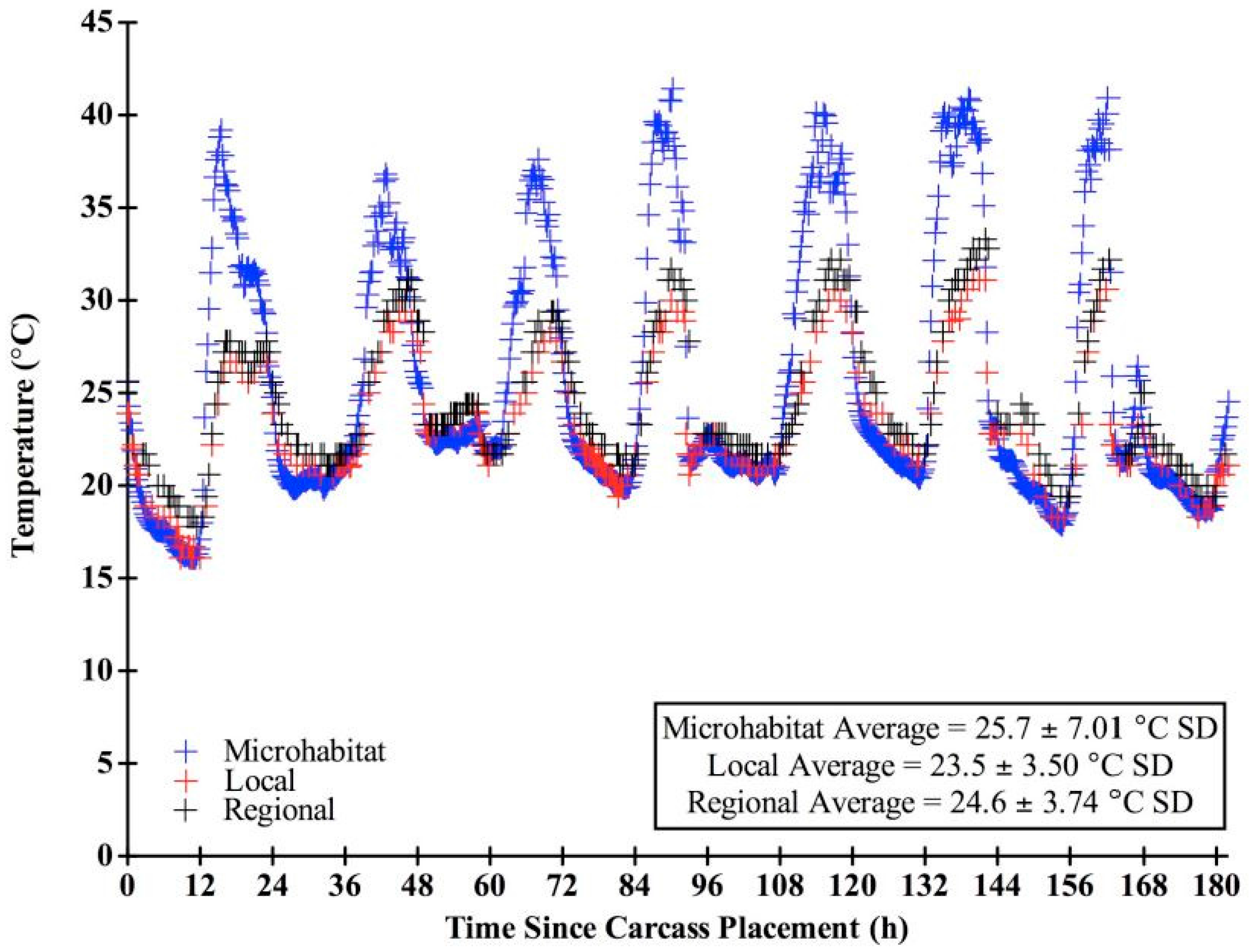
We chose “expected” blow fly developmental data sets based on the range of developmental information provided in the literature and in concordance with our field conditions. Only studies that included: (1) developmental rates of the species; (2) associated larval length data, and (3) temperatures reflected in our field study were used in our analysis. Several other data sets are available, but were not utilized here due to a lack of larval length data [47,48,49]. Other studies utilized temperatures not consistent with those measured in this study [19,49,50,51,52,53]. For instance, data sets with hourly ranges for larvae reared at 25 °C were used for both species, since the overall average temperature recorded at the carcasses throughout decomposition in this study was 25.7 °C (± 7.01 SD) (Figure 3).
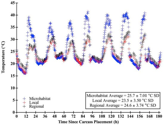
Figure 3.
Temperature (°C) throughout decomposition for the microhabitat, local, and regional sources. Microhabitat data points are every 15 min while local and regional data points represent hourly temperatures.
Actual ADH ranges were calculated by adding the hourly temperatures minus the minimum developmental threshold for each species, starting at time of carcass placement. The minimum developmental threshold was determined from previous literature: 10 °C for C. macellaria [19,50] and 6 °C for P. regina [54]. The minimum (min) and maximum (max) of actual ADH ranges match the time points when third instars were initially collected (min) and when they were last present for collection (max) for each carcass. In order to assess PCI variability, actual ADH ranges were calculated for each temperature source: the individual carcasses, the microhabitat, local, and regional temperature data. Temperature loggers of individual carcasses were used to calculate ADH ranges and PCIs in order to assess variability within the microhabitat and among replicates. Time point zero (0) represented the time when the carcasses were placed in the field, which corresponded to when the carcasses were initially exposed to potential insect colonization—approximately 4 h postmortem.
Third instar length was also utilized to calculate expected ADH values, as length can be an additional measurement used in forensic investigations. In order to understand how PCIs varied with larval length, we calculated the average 10th, 50th, and 90th percentile lengths of third instars collected from all carcasses for each calliphorid species. From these lengths, the associated ADH values were determined by visual assessment of previously published 25 °C growth curves [30,31] and minimum thresholds of 10 °C for C. macellaria [19,50] and 6 °C for P. regina [54]. Length data from previous developmental data sets were only available in line graph form [30,31], thus length to development time conversions were completed by extrapolating the length value to the growth curve above time using published recommendations of Wells and Lamotte [55] for this kind of data set. Extrapolation was to the nearest 0.25 mm.
PCI estimates were calculated as the hour ranges, for each temperature source, that correspond to the expected ADH values derived from third instar developmental stage and length data sets [30,31].
2.5. Statistical Analysis
Repeated measures analysis of variance (rm-ANOVA) was conducted to compare differences in temperature among the three spatially distinct weather data sets (microhabitat, local, regional) and among the individual carcasses [56]. Minimum, median, and maximum actual third instar ADH values among temperature sources were compared using an ANOVA. A paired t-test was performed to compare temperature differences between the local and regional sources over time, and between the actual and expected minimum, median, and maximum PCIs derived from the individual carcass temperatures. A Spearman Rank test was used to test for a correlation in the relative abundance of C. macellaria and P. regina third instars. Further, the coefficient of variation (CV) was used to represent temperature variability at each source and to represent the third instar lengths at each sampling time point for each species. All statistical tests were performed using SAS Studio 3.5 [57], and all p-values were considered significant with alpha ≤ 0.05.
3. Results
3.1. Temperature
There were significantly different (F = 10.22, df = 184, p < 0.0001) temperature means (± SD) among the microhabitat, local, and regional sources, which were 25.7 (± 7.01) °C, 23.5 (± 3.50) °C, and 24.6 (± 3.74) °C, respectively. Microhabitat temperatures were more variable (CV = 0.27) than both local (CV = 0.15) and regional (CV = 0.15) weather station temperatures. There was little variation between temperatures recorded at the local and regional sources; however, temperature differences between local and regional over time were significant (t = −12.19, df = 182, p < 0.0001). All three temperature sources recorded similar daily minimum temperatures (microhabitat: 19.5 ± 1.89 °C SD, local: 19.9 ± 2.06 °C SD, regional: 20.7 ± 1.40 °C SD). However, the microhabitat consistently recorded higher daily maximum temperatures (39.1 ± 1.65 °C SD) than the local (29.5 ± 1.56 °C SD) and regional (31.1 ± 1.89 °C SD) sources (Figure 3). There were significant mean temperature differences among the six carcasses (F = 38.31, df = 187, p < 0.0001). On average, temperature loggers of the western most carcass (N = 1: 25.4 ± 6.81 °C SD) and the eastern most carcasses (N = 2: 25.1 ± 6.53, 24.8 ± 5.64 °C SD) recorded lower temperatures than those in the center of the field (N = 3: 25.8 ± 7.32, 27.0 ± 9.38, 26.4 ± 8.38 °C SD).
3.2. Calliphoridae Larvae
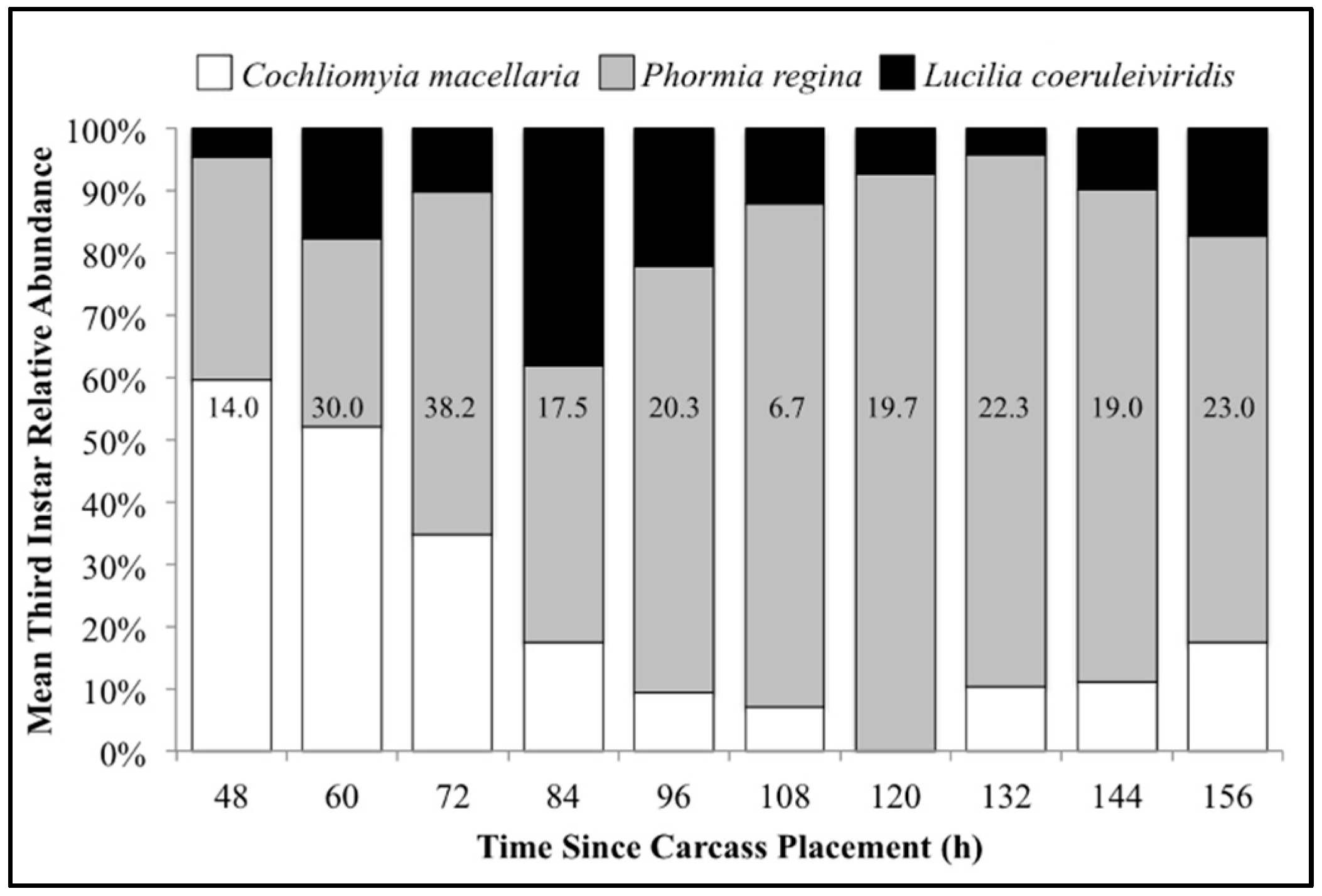
The number of carcasses sampled at each time point varied with larval mass presence or absence and resource quantity remaining among carcasses. For example, larval masses were still present on the western most carcass at 156 h following placement while, at the same time, all the larvae from the other carcasses had already migrated away from the body to begin pupation. Calliphoridae egg clutches were first observed on two carcasses in the center of the field approximately 20–30 min after placement, while all other carcasses were colonized no more than 12 h later. Third instars were first collected as early as 48 h after carcass placement and as late as 156 h. A total of 904 third instars were identified: 258 C. macellaria, 509 P. regina, and 137 Lucilia coeruleiviridis (Macquart) (Diptera: Calliphoridae) (Table S1). The relative abundances and additional data of each species can be found in our recent publication [58]. All third instar C. macellaria and P. regina were measured and used for ADH and PCI calculations. Lucilia coeruleiviridis was not utilized due to low abundance and lack of developmental data in the literature. The greatest number of C. macellaria third instars was recorded within 48–60 h following carcass placement. The abundance of P. regina increased shortly thereafter (72 h) and then decreased (84–108 h) before increasing again (120 h) (Figure 4). Cochliomyia macellaria third instar average relative abundance was greatest at 48 h (59.51%), while P. regina relative abundance remained above 60% for most of decomposition from 84–156 h (Figure 4). There was a significant negative corrleation between C. macellaria and P. regina third instar average relative abundance over time (ρ = −0.9, p = 0.0002). The average relative abundance of third instars, compared to first and second instars, generally increased over time (Figure 5).

Figure 4.
Mean relative abundance of all third instars collected throughout decomposition: Cochliomyia macellaria, Phormia regina, and Lucilia coeruleiviridis. Numbers on each column represent the average number of third instars (all species) collected at that time point.
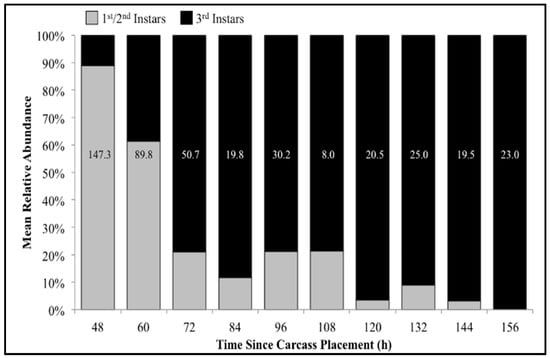
Figure 5.
Mean relative abundance of first/second (pooled) and third instars of all species collected throughout decomposition. Numbers on each column represent the average number of larvae (all instars) collected at that time point.
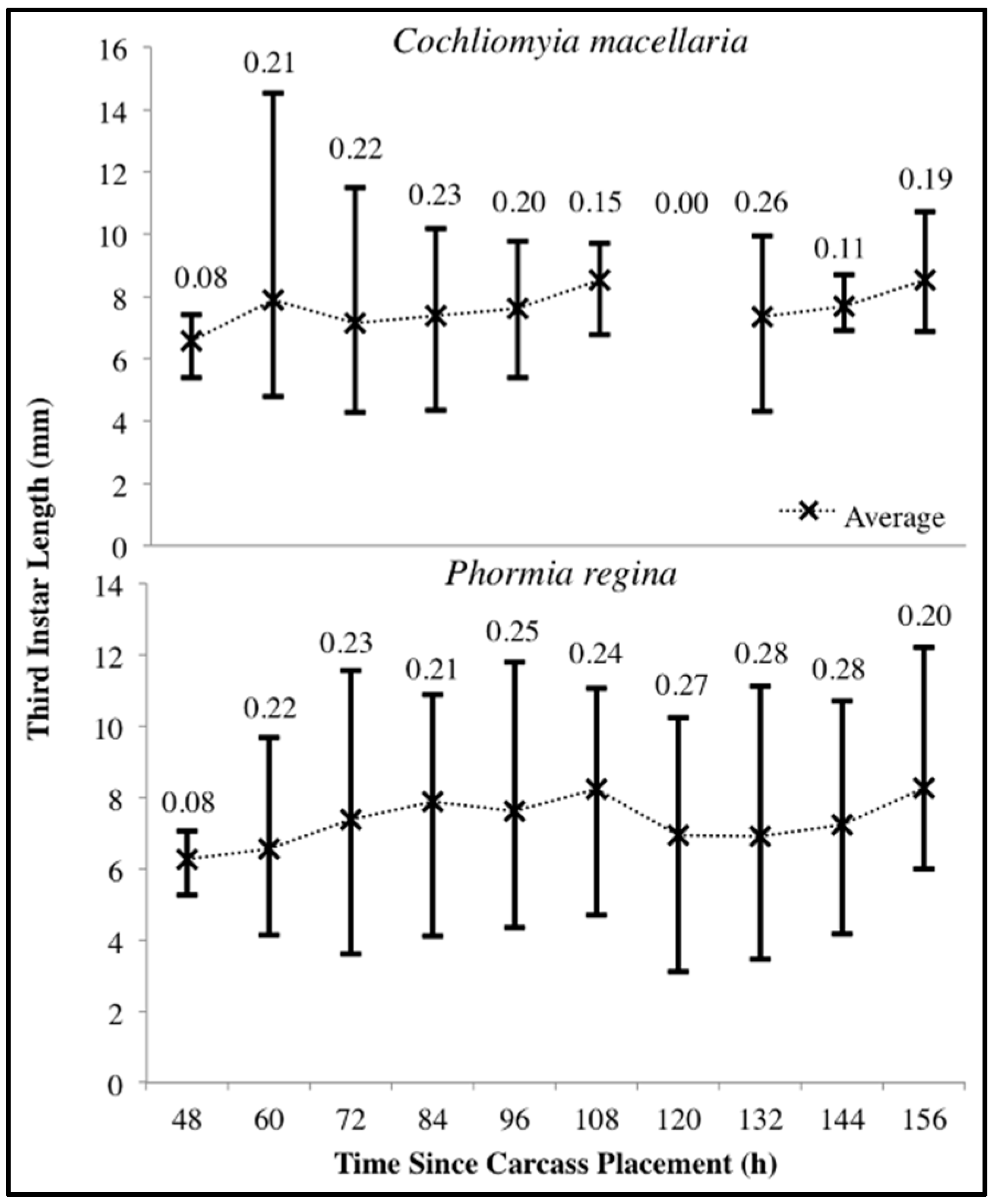
For both species there was substantial variability in third instar body lengths. The overall range of C. macellaria third instar lengths was 4.28–14.53 mm and 3.11–12.22 mm for P. regina. Even within a single sampling point, there was substantial length variability for each species. The greatest ranges within a single sampling point were 4.80–14.53 mm at 60 h and 3.62–11.55 mm at 72 h for C. macellaria and P. regina, respectively. The average (± SD) length for each species, however, changed little over time (C. macellaria: 7.63 ± 0.63 mm; P. regina: 7.33 ± 0.68 mm). The variability, represented as the CV for each time point, in third instar length fluctuated over time for C. macellaria, but the variability in P. regina remained fairly consistent throughout decomposition (Figure 6). There were significant differences among the 10th, 50th, and 90th percentile lengths for C. macellaria (F = 99.63, df = 2, p < 0.0001) and P. regina (F = 22.79, df = 2, p < 0.0001) (Table 1 and Table 2).
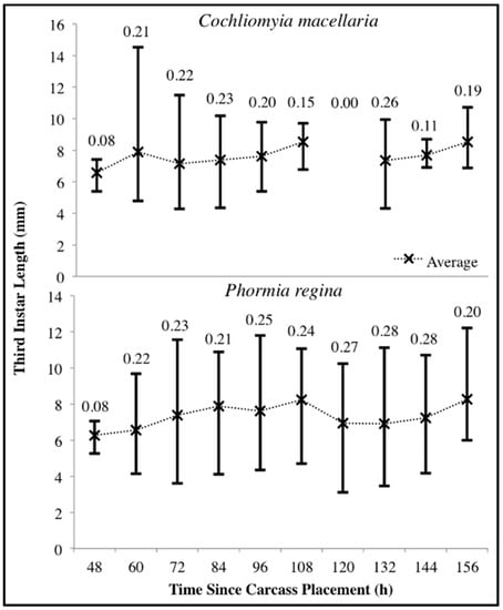
Figure 6.
Range of Cochliomyia macellaria and Phormia regina third instar body length throughout decomposition. Upper and lower limits represent the maximum and minimum lengths, respectively. Average lengths are marked with an “X”. Coefficient of variation is noted above each time point. No C. macellaria third instars were collected at 120 h following carcass placement.

Table 1.
Actual and expected minimum (Min), median (Med), and maximum (Max) accumulated degree hours (ADH) associated with Cochliomyia macellaria development, using a minimum developmental threshold of 10° C, based on third instar range (time present on carcasses) and body lengths representing the 10th, 50th, and 90th percentiles. White and green areas represent actual values while gray areas represent expected values [30].
Table 2.
Actual and expected minimum (Min), median (Med), and maximum (Max) accumulated degree hours (ADH) associated with Phormia regina development, using a minimum developmental threshold of 6° C, based on third instar range (time present on carcass) and body lengths representing the 10th, 50th, and 90th percentiles. White and green areas represent actual values while gray areas represent expected values [31].
3.3. ADH Ranges
The expected third instar ADH ranges from development data sets of Byrd and Butler [30] and Byrd and Allen [31] most often fell within the actual ADH range derived from the local temperatures for C. macellaria and regional temperatures for P. regina. For both species, microhabitat temperatures produced the widest ADH range (Figure 7 and Figure 8). The expected minimum ADH for both species, however, was greater than the actual minimum ADH for all temperature sources (C. macellaria: by 15, 120, and 63 ADH; P. regina: by 42, 157, and 99 ADH for microhabitat, local, and regional temperatures, respectively). The expected maximum ADH was less than the actual maximum ADH when microhabitat and regional temperatures were used with C. macellaria (by 284 and 130 ADH, respectively) and with microhabitat temperatures for P. regina (by 171 ADH) (Figure 7 and Figure 8). There were no significant differences for minimum, median, or maximum actual ADH among temperature sources for C. macellaria (F = 1.99, df = 3, p = 0.1473; F = 1.32, df = 3, p = 0.2947; F = 0.90, df = 3, p = 0.4604) or P. regina (F = 0.53, df = 3, p = 0.6649; F = 2.47, df = 3, p = 0.0914; F = 1.92, df = 3, p = 0.1592).
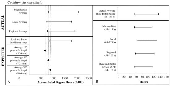
Figure 7.
Comparison of expected accumulated degree hours (ADH) associated with Cochliomyia macellaria third instar developmental stage and length to actual third instar ADH ranges calculated for each temperature source: microhabitat, local, and regional. Actual ADH ranges represent the average range among carcasses. Black diamonds represent expected ADH values derived from 10th, 50th, and 90th percentile third instar lengths (A). Comparison of the average Cochliomyia macellaria third instar post-colonization interval (PCI as hours) to estimated PCIs for each temperature source (B). For both A and B: thin horizontal lines with vertical ends represent minimum-maximum ranges and values above the thick black line are actual while those below are expected or estimated based on different temperature sources or development data set.

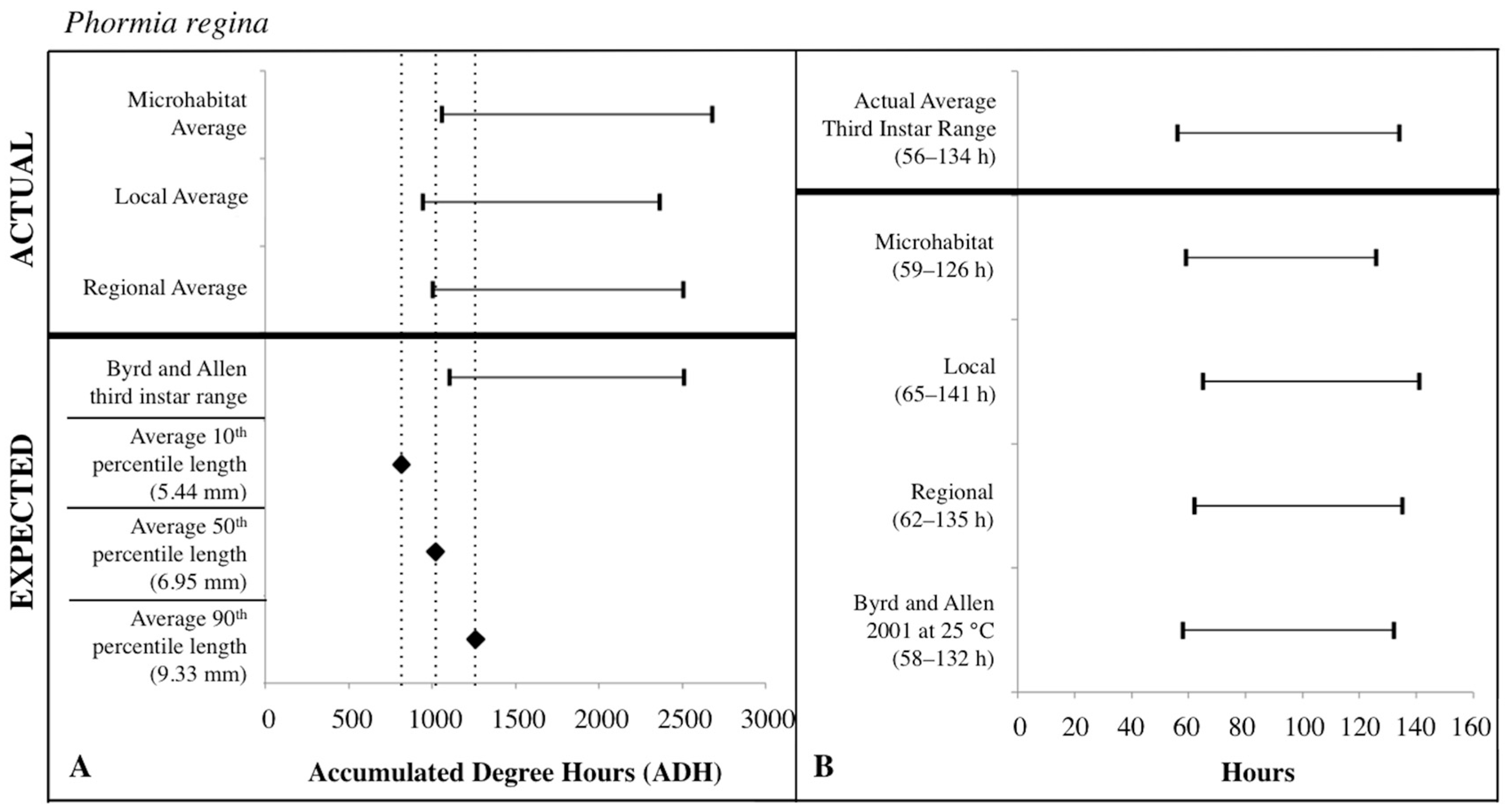
Figure 8.
Comparison of expected accumulated degree hours (ADH) associated with Phormia regina third instar developmental stage and length to actual third instar ADH ranges calculated for each temperature source: microhabitat, local, and regional. Actual ADH ranges represent the average range among carcasses. Black diamonds represent expected ADH values derived from 10th, 50th, and 90th percentile third instar lengths (A). Comparison of the average Phormia regina third instar post-colonization interval (PCI as hours) to estimated PCIs for each temperature source (B). For both A and B: thin horizontal lines with vertical ends represent minimum-maximum ranges and values above the thick black line are actual while those below are expected or estimated based on different temperature sources or development data set.
The expected third instar ADH range encompassed more of the actual ADH range when larvae from P. regina were used. For P. regina, the expected third instar ADH range accounted for 86.8%, 88.9%, and 93.4% of the actual ADH range for microhabitat, local, and regional temperatures, respectively. For C. macellaria, the expected third instar ADH range was 75.7%, 88.5%, and 82.8% of the actual ADH range for microhabitat, local, and regional temperatures, respectively. Overall, the expected ADH ranges under-represented the actual ADH range, but did encompass the average actual ADH for all temperature sources (Table 1 and Table 2).
3.4. Post-Colonization Intervals
PCI estimates for each temperature source were calculated using the expected third instar ADH range for each species and temperature data for each source. There were no significant differences between the actual and estimated PCI minimum, median, and maximum hours derived from the individual carcass temperatures for either C. macellaria (t = −0.31, df = 5, p = 0.7681; t = 1.39, df = 5, p = 0.2224; t = 1.75, df = 5, p = 0.1406) or P. regina (t = −0.79, df = 5, p = 0.4640; t = 0.67, df = 5, p = 0.5310; t = 1.52, df = 5, p = 0.1901). Following the ADH calculations, the associated PCI estimates of P. regina expected ranges encompassed more of the actual PCI ranges. For P. regina, the third instar developmental stage based PCI estimates derived from the microhabitat, local, and regional temperature data accounted for 85.9%, 88.5%, and 92.3% of the actual PCI, respectively. For C. macellaria, the third instar developmental stage based PCI estimates derived from the microhabitat, local, and regional temperature accounted for 73.1%, 84.6%, and 79.5% of the actual PCI, respectively. Overall, microhabitat temperatures produced the narrowest PCI estimates and were the least accurate source for both species. Local temperatures produced the most accurate PCI estimate for C. macellaria, while regional temperatures were most accurate for P. regina (Figure 7 and Figure 8; Table 3 and Table 4).
Table 3.
Actual and estimated Cochliomyia macellaria post-colonization intervals (PCIs) calculated using third instars and each temperature source, with a minimum developmental threshold of 10 °C. Min, med, and max represent the minimum, median, and maximum ADH value for each PCI. White areas represent actual values, while gray and blue areas represent estimated values [30].
Table 4.
Actual and estimated Phormia regina post-colonization intervals (PCIs) calculated using third instars and each temperature source, with a minimum developmental threshold of 6 °C. Min, med, and max represent the minimum, median, and maximum ADH value for each PCI. White areas represent actual values, while gray and blue areas represent estimated values [31].
For third instar length-based estimates and previous developmental data sets [30,31], mean (± SD) larval lengths at the 10th percentile (C. macellaria: 5.36 ± 0.36 mm, P. regina: 5.44 ± 0.92 mm) for both species produced expected ADH values less than the actual minimum ADH for all temperatures sources. The 50th percentile lengths (C. macellaria: 7.21 ± 0.74 mm SD, P. regina: 6.95 ± 1.18 mm SD) of both species fell within local and regional temperature ADH ranges and just under the microhabitat minimum ADH. The 90th percentile length (C. macellaria: 9.66 ± 0.42 mm SD, P. regina: 9.33 ± 0.90 mm SD) for both species fell within the range from all sources. For both species, the expected ADH associated with the 50th percentile length was similar to the actual microhabitat and regional minimum ADH values (Figure 7 and Figure 8, Table 1 and Table 2).
Similar to the ADH ranges, the average length-based PCI estimates tended to underestimate the actual PCIs. For both species, 10th percentile lengths underestimated the actual PCI for all temperature sources (C. macellaria: by 5–13 h, P. regina: by 6–13 h). PCI estimates derived from 50th percentile lengths and local and regional temperatures fell within the actual PCI for both C. macellaria and P. regina, however, individual and microhabitat temperatures underestimated the actual PCI (C. macellaria: by 2–4 h, P. regina: by 1–2 h). All PCI estimates derived from 90th percentile lengths, regardless of species or temperature source, fell within the actual PCI (Table 5 and Table 6).
Table 5.
Actual and estimated Cochliomyia macellaria post-colonization intervals (PCIs) calculated using 10th, 50th, and 90th percentile third instar lengths and each temperature source, with a minimum developmental threshold of 10 °C. Min, med, and max represent the minimum, median, and maximum hourly value for each PCI. All time values represent hours. White areas represent actual values, while gray and blue areas represent estimated values from published development data and body lengths [30].
Table 6.
Actual and estimated Phormia regina post-colonization intervals (PCIs) calculated using 10th, 50th, and 90th percentile third instar lengths and each temperature source, with a minimum developmental threshold of 6 °C. Min, med, and max represent the minimum, median, and maximum hourly value for each PCI. All time values represent hours. White areas represent actual values, while gray and blue areas represent estimated values from published development data and body lengths [31].
4. Discussion
Recently, the forensic science community has increased efforts to recognize the amount of variability in specific disciplines (e.g., trace evidence) and develop error rates [26]. Yet, it is still relatively unknown how the accuracy of using a calliphorid developmental data set to estimate a PCI varies depending on temperature source. Utilizing weather station data distant from the scene can be problematic, as possible temperature variations between the location of the station and the death scene could result in an inaccurate calculation of insect developmental time [14,32]. Archer [59] examined the accuracy of collecting scene temperatures after body removal and retrospectively correcting weather station data. In that study, often the minimum PMI estimates improved following correction, but temperature collection after body discovery is not always possible. Archer [59] urged caution when correcting data, since weather can change significantly over a short period of time. Improvement of PMI estimates was highly variable among correlation periods and in a few instances, temperature correction was associated with a decrease in estimated decomposition time accuracy. Additionally, in that excellent study only hypothetical insect data were analyzed [59].
Monthei [51] conducted a similar study to ours in Virginia in which accumulated degree days calculated from temperatures at the carcass (ambient, inside the cage, head, thorax, abdomen) and from two weather stations at different distances from the site (5.63 and 10.46 km) were used along with two P. regina developmental data sets [31,49] to estimate PMIs. The author reported that, when using Byrd and Allen’s data set [31], the furthest weather station from the study site produced the most accurate PMI estimate. When utilizing Anderson’s data set [49], however, temperatures from the head of the carcass produced the most accurate PMI estimate. Monthei postulated that this could be due to the fact that Anderson’s data came from larvae reared in masses while Byrd and Allen kept a ratio of 1.5 larvae per 1.0 g of pork [51]. Indeed, the role of larval mass heat from thermogenesis may both increase and stabilize temperatures that are best reflected in temperature conditions from weather stations; this would be a fruitful area of research comparing multiple locations in different geographic regions.
Contrary to our hypothesis, using temperature sources nearer to the carcasses did not result in increased expected ADH range accuracy or the associated estimates of the PCI. ADH ranges determined using published developmental data sets were surprisingly more similar to the actual third instar ADH ranges when weather station temperatures were used rather than temperatures from the scene. The expected ADH ranges under-represented the actual range when microhabitat temperatures were used: the ADH range using microhabitat temperatures was greater than the weather station ranges. This wider ADH range at the microhabitat may be explained by the temperature loggers being located closer to the ground (and thus exposed to increased radiant and reflective heat) than the weather stations, resulting in higher temperatures and thus more rapid accumulation of degree hours [1]. The greatest difference in temperatures between the sources occurred during the afternoon, when temperatures were highest. Additionally, developmental time is longer for C. macellaria and P. regina under cyclic temperatures than at a constant temperature [19]. This could explain why the expected ADH ranges under-represented the actual ADH ranges.
Regardless of the temperature source used to calculate ADH ranges for use in PCI estimates, we hypothesized that the artificial circumstances (i.e., controlled growth chamber) of the developmental data sets would result in differences in the estimated PCIs [30,31] compared to the actual PCIs based on 12 h interval field observations and sample collections [1]. Constant temperature conditions and other variables (e.g., humidity) of lab conditions are very different from field conditions where temperatures naturally fluctuate and development can be influenced by additional abiotic variables (e.g., precipitation). Our findings suggest that there were fewer extreme fluctuations in temperature from the weather stations than at the microhabitat, making it more similar to the laboratory setting where conditions were constant. These two sources of error—utilizing expected ADH ranges from data sets from conditions different than those experienced by larvae at the scene, and weather station temperatures that vary from those at the scene—may be canceling each other in PCI estimates: one may overestimate while the other underestimates development time [60].
Another notable finding was the variation in species and third instar length. This supports the importance of thorough evidence collection in order to utilize as much information available from a death scene as possible. The largest larvae may be the most developed and therefore an initial colonizer, but the presence of smaller third instars, of either the same or different species, could indicate multiple oviposition events that could help develop a more complete timeline of the post-colonization activity. Third instars were present for a wide range of time (hours), yet the relative abundances of this life stage compared to other instars shifted throughout decomposition. There was an increase in relative abundance of first and second instars at 96 h and then an increase in abundance of third instar P. regina at 120 h, suggesting a second oviposition event occurred later in the decomposition process [13]. Considering smaller third instars of another species collected from a body could be informative, as different species colonize at different times following death. Further, P. regina is known as a later colonizer during carrion decomposition, compared to L. coeruleiviridis, C. macellaria, and Chrysomya rufifacies (Macquart) (Diptera: Calliphoridae) [29], and prefers a resource that has been previously colonized [61]. We initially observed a high average relative abundance of C. macellaria third instars (59.51%) early on (48 h) followed by an increase in P. regina third instar average relative abundance (55.01% at 72 h) (Figure 4). Using the 50th and 90th percentile lengths of third instars was also effective at indicating the lower ADH and PCI range, but failed to encompass the upper ADH and PCI ranges. A possible explanation could be found in the preservation method. Specimens were frozen and then placed in ethanol, which could have led to shrinkages and underestimated ranges based on larval length [62]. It would be useful to replicate this study and compare PCI estimates derived from larval body length among different preservation methods. This knowledge would be valuable as experience and technique varies among investigators, and it is not uncommon for an entomologist to receive poorly preserved specimens.
Finally, the Calliphoridae collected during our study are similar to the species reported for a previous study conducted in the same geographic location [63]. This previous study also used swine carcasses and found P. regina and L. coeruleiviridis as colonizers (evident by larvae present on the carcasses) with additional blow fly species present as adults: C. macellaria, Hydroatea leucostoma (Fabricius) (Diptera: Calliphoridae), and Pollenia rudis (Fabricius) (Diptera: Calliphoridae) [63]. Phormia regina is considered a cold weather species, while C. macellaria is more abundant in warmer regions, however, both are common postmortem colonizers [30,31]. Thus, our findings are consistent with previous descriptions of the distribution and the ecology of the species that we collected in this study.
5. Conclusions
This study demonstrates that there is substantial variability in Calliphoridae species occurrence and larval development during carcass decomposition that can influence ADH-based estimates of the PCI. It further shows that the temperature source for forensic investigations using insect evidence can be highly variable, depending on the spatial location of the weather station or temperature sensor. The goal of this study was not to build predictive models for PCI or PMI based on calliphorid life history traits; however, these data do provide important insight into the potential abiotic and biotic variability that may influence the use and interpretation of calliphorid larvae evidence collected from entire carcasses (as human surrogates) in a natural habitat. Understanding these sources of variability in a natural environmental setting has the potential to inform both existing and future PMI predictive model building efforts [33,34,35]. Indeed, the importance of refining existing, or developing new, predictive models of PMI will move the discipline of forensic entomology forward and this study is only one effort to support these important endeavors. Additional studies are needed to more fully understand how variation in both biotic and abiotic factors among habitats and ecoregions can be used to develop broadly relevant and useful models in forensic entomology.
Supplementary Materials
The following are available online at http://www.mdpi.com/2075-4450/8/2/40/s1, Table S1: Number of larvae, and third instars specifically, collected per carcass at each sampling period.
Acknowledgments
The authors thank Christine Picard for her involvement in study design and Charity Owings, Elizabeth Went, and Jarrett Hiatt for their assistance in sample collection. Hadley O’Brien and Andre Yoshikawa are greatly appreciated for photographing and measuring the larvae. Funding was provided by the Michigan State University College of Agriculture and Natural Resources (Department of Entomology) and College of Osteopathic Medicine (Department of Osteopathic Medical Specialties), and Purdue Department of Entomology.
Author Contributions
Courtney R. Weatherbee, M. Eric Benbow, and Jennifer L. Pechal conceived and designed the study, data collection, and data analyses; Courtney R. Weatherbee performed the experiments; Courtney R. Weatherbee and Jennifer L. Pechal analyzed the data; Trevor Stamper and M. Eric Benbow contributed reagents/materials/analysis tools, and Trevor Stamper contributed logistical support, swine carcasses, and the secured environmental space for the study; Courtney R. Weatherbee, Jennifer L. Pechal, Trevor Stamper, and M. Eric Benbow wrote the paper.
Conflicts of Interest
The authors declare no conflict of interest. The funding sponsors had no role in the design of the study; in the collection, analyses, or interpretation of data; in the writing of the manuscript, and in the decision to publish the results.
References
- Byrd, J.H.; Castner, J.L. Forensic Entomology: The Utility of Arthropods in Legal Investigations; CRC Press: Boca Raton, FL, USA, 2010. [Google Scholar]
- Catts, E.P.; Haskell, N.H. Entomology and Death: A Procedural Guide; Joyce’s Print Shop, Inc.: Clemson, SC, USA, 1990. [Google Scholar]
- Tomberlin, J.K.; Mohr, R.; Benbow, M.E.; Tarone, A.M.; VanLaerhoven, S. A roadmap for bridging basic and applied research in forensic entomology. Annu. Rev. Entomol. 2011, 56, 401–421. [Google Scholar] [CrossRef] [PubMed]
- Amendt, J.; Campobasso, C.P.; Gaudry, E.; Reiter, C.; LeBlanc, H.N.; Hall, M.J. Best practice in forensic entomology—Standards and guidelines. Int. J. Legal Med. 2007, 121, 90–104. [Google Scholar] [CrossRef] [PubMed]
- Anderson, G.S. Comparison of decomposition rates and faunal colonization of carrion in indoor and outdoor environments. J. Forensic Sci. 2011, 56, 136–142. [Google Scholar] [CrossRef] [PubMed]
- Goff, M.L. Problems in estimation of postmortem interval resulting from wrapping of the corpse: A case study from Hawaii. J. Agric. Entomol. 1992, 9, 237–243. [Google Scholar]
- Bugajski, K.N. An Examination of the Effect of Household Chemicals on Blow Fly Oviposition, Growth, Development, and Estimations of the Post Mortem Interval. Ph.D. Thesis, Purdue University, West Lafayette, IN, USA, 2011. [Google Scholar]
- Avila, F.W.; Goff, M.L. Arthropod succession patterns onto burnt carrion in two contrasting habitats in the Hawaiian islands. J. Forensic Sci. 1998, 43, 581–586. [Google Scholar] [CrossRef] [PubMed]
- Kreitlow, K.L. Insect Succession in a Natural Environment. In Forensic Entomology: The Utility of Arthropods in Legal Investigations; Byrd, J.H., Castner, J.L., Eds.; CRC Press: Boca Raton, FL, USA, 2010; pp. 251–269. [Google Scholar]
- Merritt, R.W.; De Jong, G.D. Arthropod Communities in Terrestrial Environments. In Carrion Ecology, Evolution, and Their Applications; Benbow, M.E., Tomberlin, J.K., Tarone, A.M., Eds.; CRC Press: Boca Raton, FL, USA, 2016; pp. 65–91. [Google Scholar]
- Davidson, J. On the relationship between temperature and rate of development of insects at constant temperatures. J. Anim. Ecol. 1944, 13, 26–38. [Google Scholar] [CrossRef]
- Richards, C.S.; Villet, M.H. Data quality in thermal summation development models for forensically important blowflies. Med. Vet. Entomol. 2009, 23, 269–276. [Google Scholar] [CrossRef] [PubMed]
- Richards, C.S.; Villet, M.H. Factors affecting accuracy and precision of thermal summation models of insect development used to estimate post-mortem intervals. Int. J. Legal Med. 2008, 122, 401–408. [Google Scholar] [CrossRef] [PubMed]
- Catts, E.P. Problems in estimating the postmortem interval in death investigations. J. Agric. Entomol. 1992, 9, 245–255. [Google Scholar]
- Mahat, N.A.; Zafarina, Z.; Jayaprakash, P.T. Influence of rain and malathion on the oviposition and development of blowflies (Diptera: Calliphoridae) infesting rabbit carcasses in Kelantan, Malaysia. Forensic Sci. Int. 2009, 192, 19–28. [Google Scholar] [CrossRef] [PubMed]
- Goff, M.L.; Brown, W.A.; Omori, A.I. Preliminary observations of the effect of methamphetamine in decomposing tissues on the development rate of Parasarcophaga ruficornis (Diptera: Sarcophagidae) and implications of this effect on the estimations of postmortem intervals. J. Forensic Sci. 1992, 37, 867–872. [Google Scholar] [PubMed]
- Goff, M.L.; Brown, W.A.; Hewadikaram, K.A.; Omori, A.I. Effect of heroin in decomposing tissues on the development rate of Boettcherisca peregrina (Diptera, Sarcophagidae) and implications of this effect on estimation of postmortem intervals using arthropod development patterns. J. Forensic Sci. 1991, 36, 537–542. [Google Scholar] [CrossRef] [PubMed]
- Goff, M.L.; Omori, A.I.; Goodbrod, J.R. Effect of cocaine in tissues on the development rate of Boettcherisca peregrina (Diptera: Sarcophagidae). J. Med. Entomol. 1989, 26, 91–93. [Google Scholar] [CrossRef] [PubMed]
- Greenberg, B. Flies as forensic indicators. J. Med. Entomol. 1991, 28, 565–577. [Google Scholar] [CrossRef] [PubMed]
- Picard, C.J.; Deblois, K.; Tovar, F.; Bradley, J.L.; Johnston, J.S.; Tarone, A.M. Increasing Precision in development-based postmortem interval estimates: What‘s sex got to do with it? J. Med. Entomol. 2013, 50, 425–431. [Google Scholar] [CrossRef] [PubMed]
- Owings, C.G.; Spiegelman, C.; Tarone, A.M.; Tomberlin, J.K. Developmental variation among Cochliomyia macellaria Fabricius (Diptera: Calliphoridae) populations from three ecoregions of Texas, USA. Int. J. Legal Med. 2014, 128, 709–717. [Google Scholar] [CrossRef] [PubMed]
- Tarone, A.M.; Foran, D.R. Components of developmental plasticity in a Michigan population of Lucilia sericata (Diptera: Calliphoridae). J. Med. Entomol. 2006, 43, 1023–1033. [Google Scholar] [CrossRef] [PubMed]
- Clark, K.; Evans, L.; Wall, R. Growth rates of the blowfly, Lucilia sericata, on different body tissues. Forensic Sci. Int. 2006, 156, 145–149. [Google Scholar] [CrossRef] [PubMed]
- Ahmad, A.; Broce, A.; Zurek, L. Evaluation of significance of bacteria in larval development of Cochliomyia macellaria (Diptera: Calliphoridae). J. Med. Entomol. 2006, 43, 1129–1133. [Google Scholar] [CrossRef] [PubMed]
- Daubert v. Merrell Dow Pharmaceuticals, Inc. 1993. Available online: https://supreme.justia.com/cases/federal/us/509/579/case.html (accessed on 5 September 2015).
- National Research Council. Strengthening Forensic Science in the United States: A Path Forward. In Committee on the Judiciary House of Representatives; U.S. Government Printing Office: Washington, DC, USA, 2009. [Google Scholar]
- Tomberlin, J.K.; Benbow, M.E.; Tarone, A.M.; Mohr, R.M. Basic research in evolution and ecology enhances forensics. Trends Ecol. Evol. 2011, 26, 53–55. [Google Scholar] [CrossRef] [PubMed]
- Tomberlin, J.K.; Benbow, M.E. Forensic Entomology: International Dimensions and Frontiers; CRC Press: Boca Raton, FL, USA, 2015. [Google Scholar]
- Gruner, S.V.; Slone, D.H.; Capinera, J.L. Forensically important Calliphoridae (Diptera) associated with pig carrion in rural North-Central Florida. J. Med. Entomol. 2007, 44, 509–515. [Google Scholar] [CrossRef] [PubMed]
- Byrd, J.H.; Butler, J.F. Effects of temperature on Cochliomyia macellaria (Diptera: Calliphoridae) development. J. Med. Entomol. 1996, 33, 901–905. [Google Scholar] [CrossRef] [PubMed]
- Byrd, J.H.; Allen, J.C. The development of the black blow fly, Phormia regina (Meigen). Forensic Sci. Int. 2001, 120, 79–88. [Google Scholar] [CrossRef]
- Baker, D.G. Climate of Minnesota. Part XV, Normal Temperatures (1951–80) and Their Application. Available online: https://www.google.com.hk/url?sa=t&rct=j&q=&esrc=s&source=web&cd=2&ved=0ahUKEwj7ksOY0P3SAhXIzbwKHb7gAOQQFggfMAE&url=https%3A%2F%2Fconservancy.umn.edu%2Fbitstream%2Fhandle%2F11299%2F122927%2FSB566.pdf%3Fsequence%3D1%26isAllowed%3Dy&usg=AFQjCNHyq4xq1fhfX6iV0WxN7rDvuk1FhA (accessed on 5 September 2014).
- Baque, M.; Amendt, J. Strengthen forensic entomology in court—The need for data exploration and the validation of a generalised additive mixed model. Int. J. Legal Med. 2013, 127, 213–223. [Google Scholar] [CrossRef] [PubMed]
- Lamotte, L.R.; Wells, J.D. Inverse prediction for multivariate mixed models with standard software. Stat. Papers 2016, 57, 929–938. [Google Scholar] [CrossRef]
- Ieno, E.N.; Amendt, J.; Fremdt, H.; Saveliev, A.A.; Zuur, A.F. Analysing Forensic Entomology Data Using Additive Mixed Effects Modeling. In Current Concepts in Forensic Entomology; Amendt, J., Goff, M.L., Campobasso, C.P., Grassberger, M., Eds.; Springer: Dordrecht, The Netherlands, 2010; pp. 139–162. [Google Scholar]
- Catts, E.P.; Goff, M.L. Forensic entomology in criminal investigations. Annu. Rev. Entomol. 1992, 37, 253–272. [Google Scholar] [CrossRef] [PubMed]
- Pechal, J.L.; Crippen, T.L.; Tarone, A.M.; Lewis, A.J.; Tomberlin, J.K.; Benbow, M.E. Microbial community functional change during vertebrate carrion decomposition. PLoS ONE 2013, 8, e79035. [Google Scholar] [CrossRef] [PubMed]
- Pechal, J.L.; Benbow, M.E.; Crippen, T.L.; Tarone, A.M.; Tomberlin, J.K. Delayed insect access alters carrion decomposition and necrophagous insect community assembly. Ecosphere 2014, 5, 1–21. [Google Scholar] [CrossRef]
- Pechal, J.L.; Crippen, T.L.; Benbow, M.E.; Tarone, A.M.; Dowd, S.; Tomberlin, J.K. The potential use of bacterial community succession in forensics as described by high-throughput metagenomic sequencing. Int. J. Legal Med. 2013, 128, 193–205. [Google Scholar] [CrossRef] [PubMed]
- Benbow, M.E.; Lewis, A.J.; Tomberlin, J.K.; Pechal, J.L. Seasonal necrophagous insect community assembly during vertebrate carrion decomposition. J. Med. Entomol. 2013, 50, 440–450. [Google Scholar] [CrossRef] [PubMed]
- Gennard, D. Forensic Entomology: An Introduction; John Wiley & Sons, Ltd.: Chichester, UK, 2012. [Google Scholar]
- Smith, K.G.V. A Manual of Forensic Entomology; Cornell University Press: Ithaca, NY, USA, 1986. [Google Scholar]
- Stojanovich, C.J.; Pratt, H.D.; Bennington, E.E. Fly Larvae: Key to Some Species of Public Health Importance; U.S. Department of Health, Education, and Welfare: Atlanta, GA, USA, 1962.
- Wells, J.D.; Byrd, J.H.; Tantawi, T.I. Key to third-instar chyrsomyinae (Diptera: Calliphoridae) from carrion in the Continental United States. J. Med. Entomol. 1999, 36, 638–641. [Google Scholar] [CrossRef] [PubMed]
- Schneider, C.A.; Rasband, W.S.; Eliceiri, K.W. NIH Image to ImageJ: 25 years of image analysis. Nat. Methods 2012, 9, 671–675. [Google Scholar] [CrossRef] [PubMed]
- Anderson, G.S.; VanLaerhoven, S.L. Forensic Entomology. In The Lawyer's Guide to the Forensic Sciences; Irwin Law: Toronto, ON, Canada, 2016. [Google Scholar]
- Roe, A.L. Development modeling of Lucilia sericata and Phormia regina (Diptera: Calliphoridae). Available online: http://digitalcommons.unl.edu/natresdiss/93/ (accessed on 16 September 2015).
- Nabity, P.D.; Higley, L.G.; Heng-moss, T.M. Effects of temperature on development of Phormia regina (Diptera: Calliphoridae) and use of developmental data in determining time intervals in forensic entomology. J. Med. Entomol. 2006, 43, 1276–1286. [Google Scholar] [CrossRef] [PubMed]
- Anderson, G.S. Minimum and maximum development rates of some forensically important Calliphoridae (Diptera). J. Forensic Sci. 2000, 45, 824–832. [Google Scholar] [CrossRef] [PubMed]
- Boatright, S.A.; Tomberlin, J.K. Effects of temperature and tissue type on the development of Cochliomyia macellaria (Diptera: Calliphoridae). J. Med. Entomol. 2010, 47, 917–923. [Google Scholar] [CrossRef] [PubMed]
- Monthei, D.R. Entomotoxicological and Thermal Factors Affecting the Development of Forensically Important Flies. Ph.D. Thesis, Virginia Polytechnic Institute and State University, Blacksburg, VA, USA, 2009. [Google Scholar]
- Núñez-Vázquez, C.; Tomberlin, J.K.; Cantú-Sifuentes, M.; García-Martínez, O. Laboratory development and field validation of Phormia regina (Diptera: Calliphoridae). J. Med. Entomol. 2013, 50, 252–260. [Google Scholar] [CrossRef] [PubMed]
- Wilson, J.M.; Lafon, N.W.; Kreitlow, K.L.; Brewster, C.C.; Fell, R.D. Comparing growth of pork- and venison-reared Phormia regina (Diptera: Calliphoridae) for the application of forensic entomology to wildlife poaching. J. Med. Entomol. 2014, 51, 1067–1072. [Google Scholar] [CrossRef] [PubMed]
- VanLaerhoven, S.L. Blind validation of postmortem interval estimates using developmental rates of blow flies. Forensic Sci. Int. 2008, 180, 76–80. [Google Scholar] [CrossRef] [PubMed]
- Wells, J.D.; Lamotte, L.R. Estimating the Postmortem Interval. In Forensic Entomology: The Utility of Arthropods in legal Investigations; Byrd, J.H., Castner, J.L., Eds.; CRC Press: Boca Raton, FL, USA, 2010; pp. 367–388. [Google Scholar]
- Box, G.E.P. Some theorems on quadratic forms applied in the study of analysis of variance problems, II. effects of inequality of variance and of correlation between errors in the two-way classification. Ann. Math. Stat. 1954, 25, 484–498. [Google Scholar] [CrossRef]
- SAS Institute, Inc. SAS Studio 3.5: User's Guide; SAS Institute Inc.: Cary, NC, USA, 2016. [Google Scholar]
- Weatherbee, C.R.; Pechal, J.L.; Eric Benbow, M. The dynamic maggot mass microbiome. Ann. Entomol. Soc. Am. 2017, 110, 45–53. [Google Scholar] [CrossRef]
- Archer, M.S. The effect of time after body discovery on the accuracy of retrospective weather station ambient temperature corrections in forensic entomology. J. Forensic Sci. 2004, 49. [Google Scholar] [CrossRef]
- Higley, L.G.; Pedigo, L.P.; Ostlie, K.R. Degday: A program for calculating degree-days, and assumptions behind the degree-day approach. Environ. Entomol. 1986, 15, 999–1016. [Google Scholar] [CrossRef]
- Rosati, J.Y. Spatial and Temporal Variability in the Carrion Insect Community: Using Blow Flies (Family: Calliphoridae) as a Model System to Study Coexistence Mechanisms at Multiple Scales. Ph.D. Thesis, University of Windsor, Windsor, ON, Canada, 2014. [Google Scholar]
- Tantawi, T.I.; Greenberg, B. The effect of killing and preservative solutions on estimates of maggot age in forensic cases. J. Forensic Sci. 1993, 38, 702–707. [Google Scholar] [CrossRef] [PubMed]
- Bugajski, K.N.; Seddon, C.C.; Williams, R.E. A comparison of blow fly (Diptera: Calliphoridae) and Beetle (Coleoptera) activity on refrigerated only versus frozen-thawed pig carcasses in Indiana. J. Med. Entomol. 2011, 48, 1231–1235. [Google Scholar] [CrossRef] [PubMed]


© 2017 by the authors. Licensee MDPI, Basel, Switzerland. This article is an open access article distributed under the terms and conditions of the Creative Commons Attribution (CC BY) license (http://creativecommons.org/licenses/by/4.0/).