Abstract
Data-driven system identification procedures have recently enabled the reconstruction of governing differential equations from vibration signal recordings. In this contribution, the sparse identification of nonlinear dynamics is applied to structural dynamics of a geometrically nonlinear system. First, the methodology is validated against the forced Duffing oscillator to evaluate its robustness against noise and limited data. Then, differential equations governing the dynamics of two weakly coupled cantilever beams with base excitation are reconstructed from experimental data. Results indicate the appealing abilities of data-driven system identification: underlying equations are successfully reconstructed and (non-)linear dynamic terms are identified for two experimental setups which are comprised of a quasi-linear system and a system with impacts to replicate a piecewise hardening behavior, as commonly observed in contacts.
1. Introduction
In recent decades, the impelling need to monitor and supervise machine and structures operations has led to an increasing usage of sensors and measuring equipment. Time varying data are analyzed and processed to obtain high fidelity models able to describe and ideally predict the system behavior under varying excitations and boundary conditions [1,2,3,4,5]. To this end, many strategies have been developed for system identifications generally based on linear theory, such as modal analysis [6,7,8]. It is superfluous to note that, in a sense, all real systems are nonlinear and may be described by linear models only within some restricted ranges of the governing parameters, or under particular conditions [9,10,11]. For example, almost all engineering applications are constituted by jointed structures [12,13,14,15,16] where frictional dissipation takes place [17,18]. Contact is mediated by roughness, which is well known to introduce nonlinear stiffening behavior [19,20,21,22]. To limit, reduce, or suppress vibrations, frictional dampers are usually adopted, which in many cases exploit dry friction, and stoppers are used [12]. Hence, in the last decade, different nonlinear identification techniques have been proposed [23], among these Brunton et al. [24] have recently suggested the sparse identification of nonlinear dynamics (SINDy) approach to reconstruct the set of nonlinear ordinary differential equations (ODE) governing the system dynamics. Taking vibration recordings as an input, SINDy outputs the ODE reconstruction, i.e., a set of differential equations that describe the observed dynamics. Stender et al. [25] proposed an optimization technique which aims at automating the system reconstruction, enforcing further sparsification of the reconstructed ODEs and at the same time reducing the error. They have tested this approach extensively for a linear oscillator and for the free vibration of a Duffing oscillator.
In this work, SINDy will be used to reconstruct the dynamics of an externally-excited oscillator which shows hardening stiffness nonlinearity. In the first part of the paper, time series will be obtained numerically, integrating the equation of motion of a Duffing oscillator. Two scenarios, which are likely to happen in practical cases, will be mimicked, i.e., (i) the case where only few states are measured, and (ii) the case when noisy data are available. In the second part of the paper, the governing equations will be reconstructed starting from the time series obtained measuring the vibrations of two cantilevers which are weakly coupled and subjected to base excitation. Similarly to the Duffing oscillators, these cantilevers have been designed to experience hardening behavior due to impact against two stoppers. It will be shown that after some smoothing of the experimental data SINDy was able to reconstruct the system dynamics with good accuracy.
2. Methods
The methods used to reconstruct analytical dynamic models and their governing equations from time series with tools to optimize the identification of the system for the different configurations studied in this work are now introduced.
Sparse Identification of Nonlinear Dynamics (SINDy)
The algorithm has been introduced by Brunton et al. [24] is named sparse identification of nonlinear dynamics (SINDy); it is a method that allows the identification of nonlinear dynamical systems using sparse regression and sparse representation, see Figure 1. It is based on the assumption of sparsity of the observed dynamics: most physical systems can be described by governing equations that are rather sparse in the high-dimensional space of possible nonlinear functions. Nonlinear dynamical systems, as found in structural dynamics, can be represented as
where represents the state of the system at time t and the nonlinear function represents the dynamic constraints that define the equation of motion of the system. The function f often consists only of a few terms, making it sparse in the space of possible functions. To determine function f from data, a time history of is collected, is measured or approximated numerically from the states and they are collected in the matrices and . Next, an augmented library, consisting of candidate nonlinear functions of , is constructed; it may consists of constants, polynomials (such as ), trigonometric functions, and other terms. Each column of represents a candidate function for the right-hand side of Equation (1). Only a few of these functions are active in each row of f, so a regression problem is set up to determine the vector of coefficients that determine which nonlinear functions are active for each degree of freedom
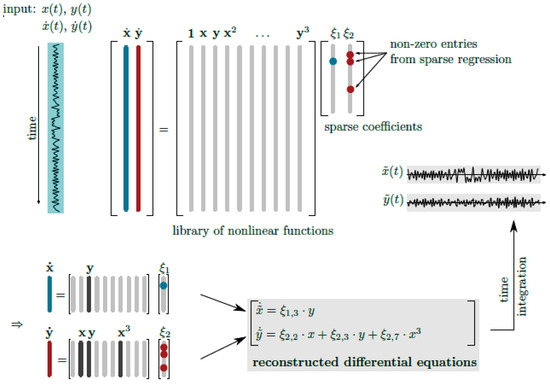
Figure 1.
Schematic illustration of the SINDy procedure. System states and their derivatives are required as time series input. Then, a library of nonlinear candidate functions is compiled. The resulting over-determined system of equations is solved by sparsity-promoting regression techniques to yield a sparse reconstruction of the underlying dynamical system in terms of ordinary differential equations. From ([25], Figure 1).
Here, the central idea is to solve the over-determined system of equations such that the coefficient vector is sparse. Hence, contrary to classical least-squares solutions, small solution terms are erased according to the sparsification parameter in an iterative fashion. As a result, each column of represents a sparse vector of coefficients determining which terms are active in the right-hand side for one of the row equations in Equation (1). Once has been determined, the reconstructed set of each row of governing equations can be read directly from it
where is a vector of symbolic functions of elements of X. Therefore, the overall model is
Each coefficient vector defines the linear combination of nonlinear functions for each state
Often, only a fraction of all states of a dynamical system can be measured during experiments; Taken’s theorem [26] allows to reconstruct the full dynamics of a nonlinear system from a single time series. The states in the reconstructed space are not, obviously, identical to states in the true phase space but the reconstructed trajectories can be useful because they are topologically similar to the original dynamics, so they have the same geometrical and dynamical properties of the measured dynamics. The strategy for state-space reconstruction is the time-delay embedding, where a single time series is re-arranged in m-dimensional reconstruction-space vectors from m time-delayed samples of the measurements . The embedding parameters are the delay , derived from the first zero of the autocorrelation function of the time series, and the embedding dimension m, estimated with the false near neighbor (FNN) algorithm, that is a standard tool for determining the embedding dimension [27,28,29].
SINDy also requires state time derivatives that can be measured or generated numerically. As proposed in [24,25]. Total Variation Regularized Numerical Differentiation (TVRegDiff) [30] is used to compute derivatives numerically without noise amplification.
SINDy tries to reconstruct the time series accurately, sometimes generating models of high complexity that reproduce the given data perfectly but rely on a larger number of active functions than the one of the actual underlying governing equation. Tools proposed by Stender et al. [25] are used to improve and automate the identification of a sparse system with SINDy. The first algorithm introduced finds a correct value of the sparsification parameter , on which the population of the coefficient matrix Ξ depends; is varied between the full range of non-zero entries (NZE) of Ξ from NZE = 100% to NZE = 0% and it selects the optimal value of the sparsification parameter that minimizes the error between the input signal and the one obtained through time integration of the identified set of ODEs. Then, an optimization is introduced to find values of coefficients that improve the reconstruction of the system; this step consists of changing the values of non-zero entries found by SINDy within prescribed boundaries and using the sequential quadratic programming (sqp) method [31] to find values that reduce the error in the reconstruction further.
In this work, the forcing terms are directly appended to the library of nonlinear functions as a column, instead of introducing an additional degree of freedom for time. In practical applications, usually the forcing is a known quantity as it is measured as a time-dependent parameter, which is reflected in the proposed setup.
3. Numerical Results
To investigate the opportunities and limitations of SINDy for geometrically nonlinear dynamical systems, the forced Duffing oscillator is studied in a first step. The dimensionless governing equation reads
where denotes the linear damping coefficient, denotes the cubic stiffness coefficient and and denote the forcing amplitude and frequency, respectively, and the derivatives with respect to the dimensionless time . Commonly, the equation of motion is transformed to a set of three first order differential equation as an autonomous dynamic system by defining the forcing as an additional system state. In this work, the forcing term are considered as an external, time-dependent input to the system, such that by introducing and a system of two first order ODE is obtained
where . Hence, considering SINDy and the library of nonlinear ansatz function, the forcing time series is appended as a column to the library of functions . In the following numerical studies, if not stated differently, this set of parameters will be considered: , , , , and initial conditions and . For the time integration, i.e., the time series generation, a time span of and a fixed sampling time of are selected. The coefficients of the monomials as found in the analytical system now read and will be referred to as the ‘reference values’ in the following sections.
This dynamical system will be used to simulate numerically different scenarios that are likely to be encountered during experimental testing: (a) missing information about all active degrees of freedom resulting from a continuum which is measured by a fixed number of sensors and (b) noise contamination from the testing environment and the measurement chain.
3.1. Complete Phase Space Information Available
In an optimal setting, all the states of the unknown dynamical system would be accessible and measured without any noise. Hence, the time series of displacement and velocity and their derivatives and are first computed numerically from integrating the Duffing Equation (6) and then provided to SINDy as inputs. Using a library of monomials up to order , a sparse dynamical system is reconstructed (see Figure 2) as described in Section 2. Table 1 reports the coefficients identified using SINDy and the reference coefficients from the analytical model in Equation (8). In fact, SINDy reconstructs the reference coefficients perfectly. Hence, also the evolution of the trajectories computed from the reconstruction is identical to the ones of the analytical model.
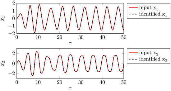
Figure 2.
Comparison of input and identified time series using polynomials up to order . As the identified system has the exact reference coefficients, there are no differences in the trajectories.

Table 1.
Comparison of coefficients for the system of equations used in the analytical model to generate the input time series and the system identified by SINDy using polynomial order and λ = 9.8168 × 10⁻¹⁸.
3.2. Noise-Contaminated Data
After testing the forced Duffing oscillator using clean—i.e., non-noisy time series—the model reconstruction performance under several levels of additive noise is studied. The time series of all system states are computed numerically from the Equation (7) and then noise is added to states and derivatives independently before giving them as inputs to SINDy. and are the state matrix and its derivatives. The dimension of each matrix is , where is the number of observations for each time series and 2 is the number of degrees of freedom. To obtain noisy data, is added to and to ; is a matrix whose dimensions are , where each column is made of normally distributed random numbers with zero mean value and unit standard deviation, while represents the noise magnitude. Different values of were studied to evaluate the quality of the reconstructions made by SINDy for increasing levels of noise. The signal-to-noise ratio (SNR) is defined as
where is the noiseless signal, is the added noise, N is the number of observations and the SNR is expressed in decibels. As an error metric the difference in the signals’ standard deviations is used. If is the reconstructed time series, the mean values are
So, their standard deviations are
The resulting error metric reads
Figure 3 displays the corresponding time domain representations of the noiseless data, of the noisy input data and the resulting dynamics of the reconstructed system given by the coefficients identified by sparse regression for (SNR = 22.33). The noiseless and reconstructed time series agree very well. SINDy turns out to be rather robust against considerable amounts of noise in the time series. The salient feature of the dynamical system—i.e., the hardening stiffness of polynomial order 3—is successfully reconstructed in the system identification, see Table 2.
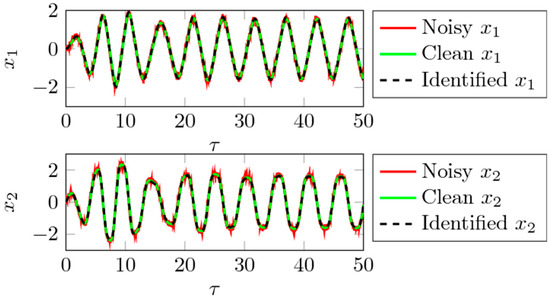
Figure 3.
Comparison of noiseless time series computed integrating equations 8, input time series with noise and time series identified by SINDy for (SNR = 22.33) resulting in error = 3.9%.
Table 2.
Coefficients of equations 8, rounded at the forth digits after the decimal point, identified by SINDy for .
The SINDy reconstruction is repeated 10 times for each value of amplitude (to account for the random noise matrix generation) and for several values of the noise magnitude to study how the error in the reconstruction increases with noise. Figure 4 depicts the evolution of the error measure (displayed as percentage) along the SNR level by box plots. The center mark labels the median value of the underlying distribution, while the lower and upper bounds of the box indicate the 25th and 75th percentiles, respectively. The dashed lines, so-called whiskers, indicate minimum and maximum values. Increasing the level of noise through the parameter the quality of the reconstruction decreases and the terms of the governing equation found differ more and more from the real ones. Additionally, the number of non-zero reconstruction terms increases along the noise level. The error falls below 5% for SNR .
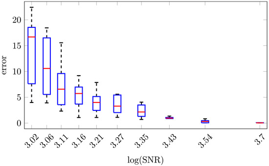
Figure 4.
Box plots of reconstruction error computed for several values of noise indicated by the SNR. The test has been iterated 10 times for each value of . MATLAB function ‘randn’ is used to compute the matrix Z used to add noise to data. The value of SNR plotted for each is the logarithm of the mean value of SNR of the 10 repetitions.
3.3. Missing Data
For the last test with time series computed numerically from the Duffing equation, only the time series of displacement are assumed as known, such as in any real experiment where only a limited number of motions can be measured. Time-delay embedding [25,26] is used to enrich the univariate data such that the phase space is reconstructed using the embedding dimension , delay to unfold the attractor in new trajectories . Generally, this procedure is a transformation into a new space, and hence the ODEs reconstructed from those data will not match the ones from the original—i.e., physical—phase space of the Duffing equation. Hence, only qualitative comparisons can be made on the coefficients and the geometry of the attractors. Supposing not to know the governing equations, it is not possible to compute the derivatives of the states analytically, so they are computed numerically using regularized derivatives as implemented in TVRegDiff [30]. Finally, the states and their derivatives are given as inputs to SINDy to reconstruct the system in the reconstructed phase space basis, see Figure 5.
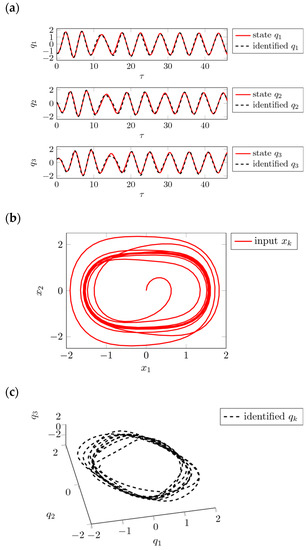
Figure 5.
Reconstruction with only displacement time series known: (a) comparison between the state in the artificial state space given as input to SINDy and its reconstruction; (b) real attractor obtained with and computed from equation 8; and (c) attractor identified by SINDy in the artificial state-space.
SINDy finds linear, cubic and forcing terms as displayed in Table 3. Hence, SINDy is conceptually able to reconstruct sets of ODEs from time-delay embedded dynamics. The loss of information that comes along with partial data, i.e., the availability of only a single state, cannot be compensated for completely by the phase space reconstruction. This behavior becomes visible in the various non-zero coefficients for a system that should only exhibit cubic characteristics. The identified system shows a similar attractor as the time-delay embedded trajectories, i.e., the system identification can be considered successful.
Table 3.
Coefficients, larger than and rounded at the fourth digit after the decimal point, found by SINDy in the identification of the governing equations starting from .
4. Investigation of Experimental Data
In the previous paragraph, SINDy was used to reconstruct the governing equations of a Duffing oscillator. Three scenarios were studied, i.e., (i) when full phase space information are available, (ii) when some states are missing and (iii) when the data are altered by noise. In this section, the governing equations will be reconstructed starting from the time series measured in a double cantilever system that is subjected to base excitation. The experimental test rig mimics the Duffing behavior as, above a certain vibration amplitude, the cantilever impact two stoppers, placed symmetrically with respect to the beam axis, which give them a piecewise linear hardening behavior.
4.1. Experimental Setup
The physical system is constituted of two clamped-free cantilevers coupled to each other by a slander connection and with masses attached at the tip of each blade and subjected to base excitation, see Figure 6. The structure was machined by means of electric erosion from a 1.5 mm thick aluminum sheet. Moreover, two masses of 32.75 g each were glued at the tip of each beam in order to reduce the frequency of the first and the second bending mode of the structure. The dimensions of the system are indicated in Figure 6a.
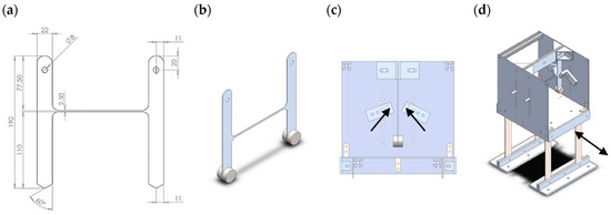
Figure 6.
Panel (a) depicts the technical drawings with all relevant dimensions in (mm) and panel (b) depicts an isometric illustration of the two beams with added masses at the tips. The beams will be clamped at their upper end. (c) rigid stoppers indicated by arrows near one beam of the system; panel (d) shows an isometric view of the whole assembly with the forcing indicated by an arrow.
The hardening behavior is introduced through two rigid stoppers, which are placed symmetrically with respect to the cantilever rest position so that the impacts are experienced for both positive and negative displacements, see Figure 6c,d. Above a certain vibration amplitude the beams touch the stoppers which instantaneously reduce the cantilever free vibration length causing a step increase in the cantilevers stiffness. The two beams are clamped to an ideally rigid frame, which is connected to a shaker. Figure 7 shows the test rig and the cantilever with an accelerometer mounted on its tip. The shaker excited the rigid frame at different frequencies and for different magnitudes of the forcing level; first the linear regime where the vibration amplitude is smaller than the gap, such that no impact happens, will be considered, and secondly the nonlinear regime where the amplitude is large enough for at least one cantilever to touch the stoppers. The time-domain measurements are obtained through accelerometers attached to the base and to the tips of the two beams.
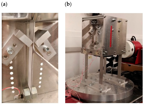
Figure 7.
Test rig for geometrically nonlinear structural dynamics of weakly coupled oscillators. Panel (a) depicts the stoppers near one of the two beams, while panel (b) shows the platform connected to the shaker.
In the linear case (Figure 8a), i.e., when there is no contact between the blades and the stoppers, both blades oscillate in phase and with a 90° phase shift with respect to the excitation. The oscillations are mono-harmonic with a maximum acceleration of . The noise contamination is low, which results in smooth time series of the accelerations. Three different states can be distinguished in the nonlinear regime—i.e., panel (b)—only the first cantilever touches the stoppers and vibrates with a much higher amplitude with respect to the second cantilever (a factor ), panel (c) is similar to (b) but with the vibration localized on the second cantilever and panel (d) where both the cantilever touch the stoppers. Similarly to the linear case, when both the cantilevers touch the stoppers, they oscillate in phase and with a 90° phase shift with respect to to the excitation. In contrast to the linear case, higher accelerations are measured, up to . These contacts result in vibro-impact-type dynamics that become visible in the fluctuations about a mono-harmonic carrier oscillation in Figure 8d. Notice that for all panels the excitation frequency is Hz and the base acceleration amplitude m/s2 respectively for panels (a,b,c,d). Those measurements clearly show that nonlinear localization and solution multiplicity may appear in nonlinear systems experiencing hardening type stiffness nonlinearities, as it was shown in [32,33], and in nonlinearly damped structures [34,35].
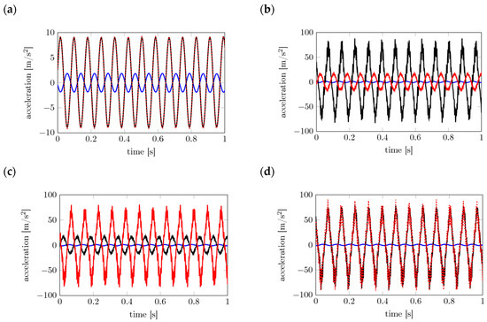
Figure 8.
Accelerations measured in time-domain. Panel (a) displays the linear regime, i.e., without contact to the stoppers (base acceleration amplitude m/s2), panel (b) depicts the localized state when just one beam touch the stoppers (base acceleration amplitude m/s2), while the panel (c) displays the case when only the second beam vibrates in large amplitudes (base acceleration amplitude m/s2). Panel (d) depicts the homogeneous state when both beams touch the stopper (base acceleration amplitude m/s2). All panels show in black measurement for the first beam, while the red lines are the same quantities for the second one. Blue lines depict the base acceleration, which for panel (a, b, c, d) respectively has amplitude m/s2 and frequency Hz.
Next, SINDy is employed to identify the governing equations of the experimental system through sparse regression. In the current setup, accelerations are measured at the tips of the two beams and of the base. It was chosen not to numerically integrate the accelerations to arrive at the corresponding velocities and displacements, as the measurements are noise-contaminated to a certain degree. Instead, the acceleration was used as state input to the system identification. Owing to the partial availability of data, embedding has to be performed anyway, which transforms the data from physical space to the embedding phase space spanned by , which unfortunately is not directly interpretable in terms of physical coefficients.
4.2. Experimental Study 1: Forced Vibration of the Beams without Impacts
In the first analysis of the linear configuration—i.e., blade dynamics without stopper impact—a high-precision reconstruction model is obtained for linear ansatz functions and a two-dimensional embedding of the acceleration time series of the first blade, see Figure 9 and Table 4. Since both blades oscillate in phase with infinitesimal differences, they are considered to be uncoupled. Hence, only the dynamics of a single blade are being studied. The reconstructed model exhibits a simple, hence sparse, structure where the excitation is acting on the second DOF. To confirm the assumption of linear dynamics as stated initially and identified in the first model, also ansatz functions of higher order were studied. However, these higher order terms vanish, compare Figure 10 and Table 5, in the reconstruction. In fact, the dynamics observed in the first study represent a linear dynamic system with external forcing.
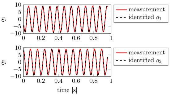
Figure 9.
Experimental study 1: Input states and obtained from time delay embedding with from the first beam acceleration time series and the resulting reconstruction using polynomials up to p = 1 and .
Table 4.
Coefficients found by SINDy for the experimental study 1 using first-order polynomials.
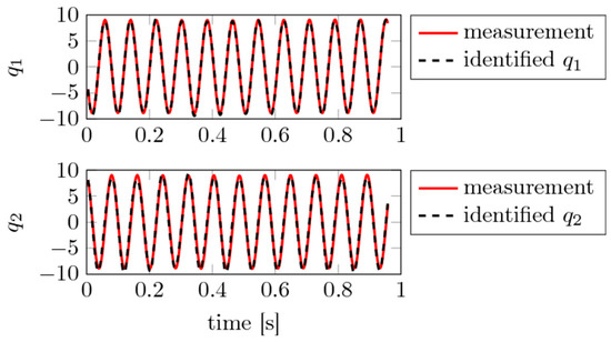
Figure 10.
Experimental study 1: Input states and obtained from time delay embedding with from the first beam acceleration time series and the resulting reconstruction using polynomials up to p = 2 and .
Table 5.
Coefficients found by SINDy for the experimental study 1 using second-order polynomials.
4.3. Experimental Study 2: Forced Vibrations of the Beams with Single-Sided Impact
In the second scenario, localized vibrations are observed, such that the blades need to be understood as being coupled. First trials using the embedded states of both blades and the excitation into account failed to produce sparse and precise ODEs. Even for different polynomial orders, temporal sampling, higher embeddings, and other tuning knobs of the SINDy indentification procedure, these issues remained. As a solution, relative motions are computed as the difference between each blade and the excitation. To deal with the vibro-impact like dynamics and the resulting amplification of the derivatives, spectral filtering was applied to the measured signals to filter out higher-frequency content above 50Hz. The resulting accelerations are embedded in two dimensions and fed to SINDy, which results in a successful reconstruction model, see Figure 11 and Table 6. The most precise model is obtained for first-order polynomials, which results in a rather fully populated coefficient matrix. and stem from the blade that touches the stoppers. The governing equations for these states are fully connected to all other states, while the not-touching states and show a sparse ODE pattern. Similar behavior was found for the case where the high-amplitude vibrations are localized in the second blade.
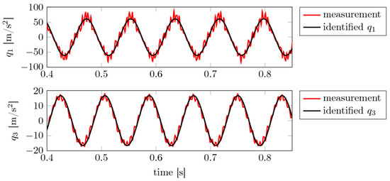
Figure 11.
Experimental study 2: Measured and identified states and using , polynomials up to p = 1 and . The signals were upsampled to .
Table 6.
Coefficients found by SINDy for the experimental study 2 using first-order polynomials. States represent relative motions between excitation and both blades, hence the excitation is not added to the nonlinear function library.
Essentially, the signal pre-filtering and successive SINDy system identification allows to capture the main vibration behavior in the form of the forced vibration of the blades. Hence, also the identified set of ODEs is comprised of linear terms while the complete system including the contacts is nonlinear. The contact-induced impact excitations are not covered here and remain as a subject for future work.
4.4. Experimental Study 3: Forced Vibration of the Beams with Both-Sided Impact
Finally, the case of uniform motion with contact of both blades is studied. Analogously to experimental study 1, the signals show almost no phase shift between the two blades such that again only the motion of the first blade is studied (the blades vibrate in-phase). Again, spectral pre-filtering was necessary for a successful application of SINDy. Best results were obtained from simple ansatz functions of first order, see Figure 12 and Table 7. The main vibration mode is met with good agreement, and hence represents a smoothed version of the measured dynamics.
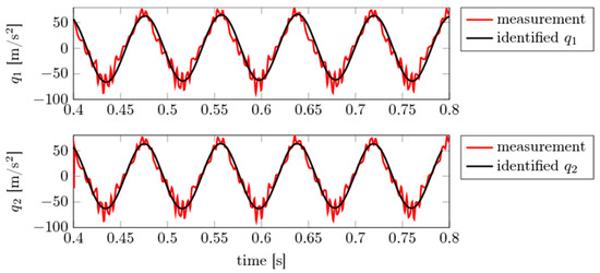
Figure 12.
Experimental study 3: Input and identified states and using , polynomials up to p = 1 and .
Table 7.
Coefficients, rounded at the second digit after the decimal point, found by SINDy in the identification of the governing equations starting from .
Compared to experimental study 1—i.e., the case of non-touching blades—the ODE for the first DOF is very similar with respect to structure and numeric values. The ODE for the second state is fully populated for the touching case considered here, thus representing more complex dynamical behavior that has to be captured by SINDy.
5. Discussion and Conclusions
The sparse identification of nonlinear dynamics (SINDy) approach has been used to reconstruct the governing equation of systems with nonlinear stiffness behavior and impacts. In the first part of the paper the equation of motion of a Duffing oscillator were integrated numerically. Contrary to the case when the full phase space information are available, in real experiments it is expected that (i) not all the states of the system can be measured and (ii) noisy data are usually available. These two scenarios have been simulated numerically showing that for missing data, by using time delay embedding, SINDy was able to reconstruct the system dynamics in a satisfactory manner. The drawback of the embedding procedure is that it is difficult to physically interpret the obtained governing equations. In case of noisy data, it has been shown that the reconstruction turns to be less accurate as noise is increased. Nevertheless, for moderate noise level (SNR greater than about 20) a faithful reconstruction of the governing equations was obtained with excellent results for SNR > 30.
In the second part of the paper the data obtained from an experimental test rig constituted by two cantilevers subjected to base excitation and impacts were considered. The measured accelerations were used to reconstruct the system dynamics and, after some smoothing operations, the time series were provided to SINDy which reconstructed the system dynamics with a good degree of approximation.
In conclusion, this preliminary study showed that SINDy could be beneficial in the future to reconstruct the dynamics of highly nonlinear systems even in presence of highly nonlinear impulsive forces, or when, in practical situations, not all the states are measured, and those which are measured are affected by measurements noise. SINDy performed well in these situations, hence this tool may be important in practical engineering applications. Based on the promising results obtained in this preliminary study, we are working to improve our experimental set-up so that not only accelerations but also displacements will be measured in the future. This will permit to deep dive into the differential equations reconstructions starting from experimentally measured time series and physically interpret the reconstructed equations. Even if the fundamental oscillation has been captured also for real systems with impacts, further work is needed to allow SINDy to capture the high frequency content introduced by impulsive forces.
Author Contributions
A.P. and M.S. conceived the study. F.F. conducted the experimental investigations. M.D. and M.S. did the numerical investigations. M.D., A.P., and M.S. wrote the manuscript. M.C. and N.H. supervised the project. All authors reviewed the work up to its final form.
Funding
A.P. is thankful to the Deutsche Forschungsgemeinschaft (DFG, German Research Foundation) for funding the project PA 3303/1-1. M.C. is supported by the Italian Ministry of Education, University and Research (MIUR) under the Departments of Excellence grant no. L.232/2016. M.S. is supported by the Deutsche Forschungsgemeinschaft (DFG, German Research Foundation) through grant no. Ho 3852/12-1. This work was funded by the Deutsche Forschungsgemeinschaft (DFG, German Research Foundation)—Projektnummer 392323616 and the Hamburg University of Technology (TUHH) in the funding programme Open Access Publishing.
Acknowledgments
The authors thank Loic Salles (Imperial College London), Aurélien Grolet (ENSAM Lille), Jeanne Auvray (Centrale Marseille) and Alessandra Vizzaccaro (Imperial College London) for funding, designing and setting up the rig from which the vibration measurements were obtained.
Conflicts of Interest
The authors declare no conflict of interest. The funders had no role in the design of the study; in the collection, analyses, or interpretation of data; in the writing of the manuscript, or in the decision to publish the results.
References
- Ondra, V.; Sever, I.A.; Schwingshackl, C.W. A method for non-parameteric identification of nonlinear vibration systems with asymmetric restoring forces from a resonant decay response. Mech. Syst. Signal Process. 2019, 114, 239–258. [Google Scholar] [CrossRef]
- Ondra, V.; Sever, I.A.; Schwingshackl, C.W. A method for detection and characterisation of structural nonlinearities using the Hilbert transform. Mech. Syst. Signal Process. 2017, 83, 210–227. [Google Scholar] [CrossRef]
- Pesaresi, L.; Stender, M.; Ruffini, V.; Schwingshackl, C.W. DIC Measurement of the Kinematics of a Friction Damper for Turbine Applications. In Dynamics of Coupled Structures; Conference Proceedings of the Society for Experimental Mechanics Series; Springer: Cham, Switzerland, 2017; Volume 4, pp. 93–101. [Google Scholar]
- Kurt, M.; Chen, H.; Lee, Y.; McFarland, M.; Bergman, L.; Vakakis, A. Nonlinear system identification of the dynamics of a vibro-impact beam: Numerical results. Arch. Appl. Mech. 2012, 82, 1461–1479. [Google Scholar] [CrossRef]
- Stender, M.; Oberst, S.; Tiedemann, M.; Hoffmann, N. Complex machine dynamics: Systematic recurrence quantification analysis of disk brake vibration data. Nonlinear Dyn. 2019, 98, 1–15. [Google Scholar] [CrossRef]
- Ewins, D.J.; Gleeson, P.T. A method for modal identification of lightly damped structures. J. Sound Vib. 1982, 84, 57–79. [Google Scholar] [CrossRef]
- Farrar, C.R.; James III, G.H. System identification from ambient vibration measurements on a bridge. J. Sound Vib. 1997, 205, 1–18. [Google Scholar] [CrossRef]
- Agbabian, M.S.; Masri, S.F.; Miller, R.K.; Caughey, T.K. System identification approach to detection of structural changes. J. Eng. Mech. 1991, 117, 370–390. [Google Scholar] [CrossRef]
- Massi, F.; Baillet, L.; Giannini, O.; Sestieri, A. Brake squeal: Linear and nonlinear numerical approaches. Mech. Syst. Signal Process. 2007, 21, 2374–2393. [Google Scholar] [CrossRef]
- Brunetti, J.; D’Ambrogio, W.; Fregolent, A. Dynamic substructuring with a sliding contact interface. Dyn. Coupled Struct. 2018, 4, 105–116. [Google Scholar]
- Stender, M.; Tiedemann, M.; Hoffmann, L.; Hoffmann, N. Determining growth rates of instabilities from time-series vibration data: Methods and applications for brake squeal. Mech. Syst. Signal Process. 2019, 129, 250–264. [Google Scholar] [CrossRef]
- Brake, M.R. (Ed.) The Mechanics of Jointed Structures: Recent Research and Open Challenges for Developing Predictive Models for Structural Dynamics; Springer: Berlin/Heidelberg, Germany, 2017. [Google Scholar]
- Tiedemann, M.; Kruse, S.; Hoffmann, N. Dominant damping effects in friction brake noise, vibration and harshness: The relevance of joints. Proc. Inst. Mech. Eng. Part D J. Automob. Eng. 2015, 229, 728–734. [Google Scholar] [CrossRef]
- Padmanabhan, K.K.; Murty, A.S.R. Damping in structural joints subjected to tangential loads. Proc. Inst. Mech. Eng. Part C Mech. Eng. Sci. 1991, 205, 121–129. [Google Scholar] [CrossRef]
- Stender, M.; Papangelo, A.; Allen, M.; Brake, M.; Schwingshackl, C.; Tiedemann, M. Structural design with joints for maximum dissipation. Shock Vib. Aircr. Aerosp. Energy Harvest. Acoust. Opt. 2016, 9, 179–187. [Google Scholar]
- Papangelo, A.; Ciavarella, M. Effect of normal load variation on the frictional behavior of a simple Coulomb frictional oscillator. J. Sound Vib. 2015, 348, 282–293. [Google Scholar] [CrossRef]
- Tonazzi, D.; Massi, F.; Baillet, L.; Brunetti, J.; Berthier, Y. Interaction between contact behaviour and vibrational response for dry contact system. Mech. Syst. Signal Process. 2018, 110, 110–121. [Google Scholar] [CrossRef]
- Tonazzi, D.; Massi, F.; Culla, A.; Baillet, L.; Fregolent, A.; Berthier, Y. Instability scenarios between elastic media under frictional contact. Mech. Syst. Signal Process. 2013, 40, 754–766. [Google Scholar] [CrossRef]
- Shi, X.; Polycarpou, A.A. Measurement and modeling of normal contact stiffness and contact damping at the meso scale. J. Vib. Acoust. 2005, 127, 52–60. [Google Scholar] [CrossRef]
- Hess, D.P.; Wagh, N.J. Evaluating surface roughness from contact vibrations. J. Tribol. 1995, 117, 60–64. [Google Scholar] [CrossRef]
- Papangelo, A.; Hoffmann, N.; Ciavarella, M. Load-separation curves for the contact of self-affine rough surfaces. Sci. Rep. 2017, 7, 6900. [Google Scholar] [CrossRef]
- Massi, F.; Berthier, Y.; Baillet, L. Contact surface topography and system dynamics of brake squeal. Wear 2008, 265, 1784–1792. [Google Scholar] [CrossRef]
- Noël, J.P.; Kerschen, G. Nonlinear system identification in structural dynamics: 10 more years of progress. Mech. Syst. Signal Process. 2017, 83, 2–35. [Google Scholar] [CrossRef]
- Brunton, S.L.; Proctor, J.L.; Kutz, J.N. Discovering governing equations from data by sparse identification of nonlinear dynamical systems. Proc. Natl. Acad. Sci. USA 2016, 113, 3932–3937. [Google Scholar] [CrossRef]
- Stender, M.; Oberst, S.; Hoffmann, N. Recovery of differential equations from impulse response time series data for model identification and feature extraction. Vibration 2019, 2, 25–46. [Google Scholar] [CrossRef]
- Takens, F. Detecting strange attractors in turbulence. In Dynamical Systems and Turbulence, Warwick: Lecture Notes in Mathematics; Springer: Berlin/Heidelberg, Germany, 1981; Volume 898, pp. 366–381. [Google Scholar]
- Oberst, S.; Lai, J.C. A statistical approach to estimate the Lyapunov spectrum in disc brake squeal. J. Vib. 2015, 334, 120–135. [Google Scholar] [CrossRef]
- Abarbanel, H.D.I.; Brown, R.; Sidorowich, J.J.; Tsimring, L.S. The analysis of observed chaotic data in physical systems. Rev. Mod. Phys. 1993, 65, 1331–1392. [Google Scholar] [CrossRef]
- Kennel, M.B.; Brown, R.; Abarbanel, H.D.I. Determining embedding dimension for phase-space reconstruction using a geometrical construction. Phys. Rev. A 1992, 45, 3403–3411. [Google Scholar] [CrossRef]
- Chartrand, R. Numerical Differentiation of Noisy, Nonsmooth Data. ISRN Appl. Math. 2011. [Google Scholar] [CrossRef]
- Nocedal, J.; Wright, S. Numerical Optimization; Springer Science & Business Media: Berlin, Germany, 2006. [Google Scholar]
- Papangelo, A.; Fontanela, F.; Grolet, A.; Ciavarella, M.; Hoffmann, N. Multistability and localization in forced cyclic symmetric structures modelled by weakly-coupled Duffing oscillators. J. Sound Vib. 2019, 440, 202–211. [Google Scholar] [CrossRef]
- Fontanela, F.; Grolet, A.; Salles, L.; Chabchoub, A.; Hoffmann, N. Dark solitons, modulation instability and breathers in a chain of weakly nonlinear oscillators with cyclic symmetry. J. Sound Vib. 2018, 413, 467–481. [Google Scholar] [CrossRef]
- Papangelo, A.; Hoffmann, N.; Grolet, A.; Stender, M.; Ciavarella, M. Multiple spatially localized dynamical states in friction-excited oscillator chains. J. Sound Vib. 2018, 417, 56–64. [Google Scholar] [CrossRef]
- Papangelo, A.; Grolet, A.; Salles, L.; Hoffmann, N.; Ciavarella, M. Snaking bifurcations in a self-excited oscillator chain with cyclic symmetry. Commun. Nonlinear Sci. Numer. Simul. 2017, 44, 108–119. [Google Scholar] [CrossRef]


© 2019 by the authors. Licensee MDPI, Basel, Switzerland. This article is an open access article distributed under the terms and conditions of the Creative Commons Attribution (CC BY) license (http://creativecommons.org/licenses/by/4.0/).