Non Smooth Contact Dynamics Approach for Mechanical Systems Subjected to Friction-Induced Vibration

Abstract

The modeling of contact is one of the main features of contact dynamics in the context of friction-induced vibrations. It can have a strong impact on the numerical results and consequently on the design choices during the optimization or specification of industrial mechanical systems. This is particularly the case for scientific studies interested in brake squeal. The objective of the paper is to recall and to promote developments concerning the use of non smooth contact dynamics approach for numerical simulations based on finite element method. The specific problem of the prediction of self-excited vibration in the context of brake squeal is discussed. In order to illustrate the potential benefit for the mechanical community of using formulations and theoretical developments from the mathematical community, the stability analysis and the estimation of nonlinear vibrations of a brake system with multiple frictional interface is investigated.

1. Introduction

The problem of friction-induced vibrations and squeal noise [1,2,3] generated by disc brakes is still nowadays a source of discomfort leading to important industrial and academic efforts for a better characterization and understanding of this phenomenon. Even if one of the main difficulty in the domain for industry and academia is to define a tool to perform numerical simulation able to calculate the stability of brake systems as well as the transient nonlinear vibration of squeal instability, one of the most important issues concerns the contact formulations and the adapted numerical solving for squeal simulations. Thereby, one of the scientific exploration pathways concerns more particularly the modeling of contact dynamics and its impact on the generation of friction-induced vibration. The investigation of the origin and the main features of contact dynamics for squeal phenomena are part of a goal of improving the understanding of squeal occurrences and promoting new brake design based on advanced consideration of pad/disc interfaces.

Two trends can be clearly distinguished for contact modeling strategies. The first representation strategy considers that the contact between two bodies is perfect without interpenetration. This idealized contact problem was posed by Signorini in 1933 [4]. The classical Signorini problem involves satisfying equalities or inequalities for two alternative sets of boundary conditions at each contact point. The second representation strategy is based on the fact that a level of interpenetration between two bodies is authorized. This corresponds to the most commonly used formulation to model and solve the problem of friction-induced vibrations due to the fact that this second modeling choice is more adaptable and functional. It finds more particularly its origin and its justification on experimental observations where contact stiffness is function of the interpenetration between bodies [5]. On the other hand, it has the disadvantage of requiring a knowledge or a fine measurement of contact stiffnesses for all contact surfaces between two bodies. This second choice for contact modeling has often been favored from a numerical point of view since the implementation of functional contact laws are easier than the Signorini formulation for the use of classical non-linear algorithms and the prediction of nonlinear vibration of mechanical systems subjected to friction-induced vibrations. Conversely, no mechanical parameter has to be identified or readjusted if the Signorini contact law is preferred. This last point is one of the main reasons that explains its use even if its numerical implementation requires specific algorithms.

Some mechanical researchers working in the field of friction-induced vibration have made the choice to consider the Signorini problem with Coulomb friction. Lorang et al. [6,7] proposed a theoretical and numerical discussion on the flutter instability of the disc-brake system of a TGV train under the contact and Coulomb friction. They also compared numerical results with measurements. Brizard et al. [8] studied performances of some reduced bases for the stability analysis of a disc/pads system in sliding contact. Loyer et al. [9] proposed a complete study on the stability analysis and the prediction of nonlinear behaviors of a sliding elastic layer for different operating conditions. Sinou et al. [10] presented a global strategy based on experiments and simulations for prediction of both squeal occurrences and nonlinear self-sustained vibrations on an industrial railway brake system. Charroyer et al. [11] studied the flutter instability for a non-smooth contact dynamical system with planar friction. They also proposed the use of the shooting method in order to determine periodic solutions of a self-excited mechanical system subject to friction-induced vibrations [12]. Lai et al. [13] discussed the use of a numerical strategy in order to efficiently compute dynamic transient solutions of rolling/sliding contact systems at high frequencies. Such works not only attempt to demonstrate the feasibility of considering the Signorini problem with Coulomb friction in mechanical applications and the importance of contact dynamics at the origin of squeal phenomena, but also to illustrate and to promote the potential interactions and collaborations between mechanical and mathematical communities.

Thus the main objective of this paper is to discuss physical modeling and numerical developments concerning the use of non smooth contact dynamics approach in the context of complex phenomena like brake squeal. Particular attention is paid to the prediction of brake squeal via numerical simulations based on finite element method. This review article is divided into four sections. Firstly, the physical modeling and mathematical formulation for solving complex mechanical problems of friction-induced vibrations with non smooth contact are presented. Secondly, the associated finite element formulation and the solving of such discretized problem for the determination of the quasi-static equilibrium, the stability of the mechanical system, as well as the prediction of the transient and self-excited vibrations are discussed. Finally, an illustration on the use of non smooth contact formulation in the context of brake squeal is proposed in detail focusing in particular on the contact dynamics at the frictional interfaces and its links with the generation of self-excited vibrations.

2. Physical Modeling and Mathematical Formulation

2.1. Unilateral Contact Laws

To deal with unilateral contact between two bodies, a geometric condition of non-penetration between the two bodies, a static condition of non-tension as well as a mechanical complementarity condition have to be defined. These three conditions can be written as a non-regularized Signorini law [4]:

$$\left\{\begin{array}{c}{u}_n-g\le 0\hfill \\ r_n\le 0\hfill \\ \left(u_n-g\right)r_n=0\hfill \end{array}\right.$$

(1)

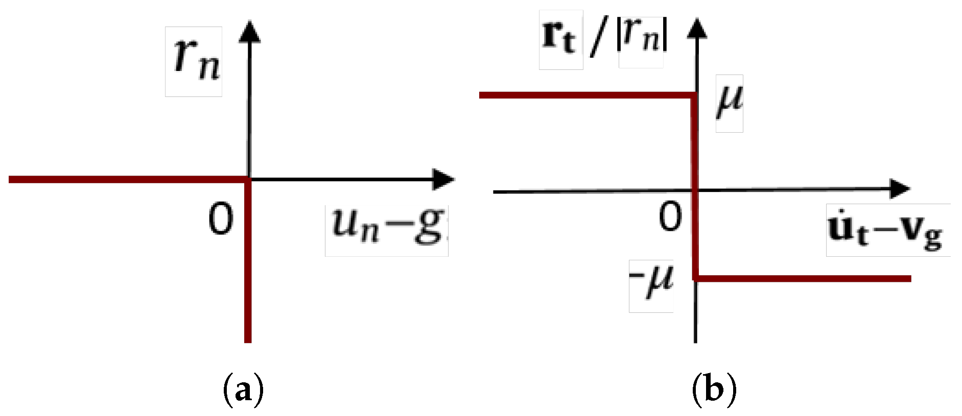
where $u_n$, g and $r_n$ are respectively the normal relative displacement, the initial gap at the contact interface and the normal contact stress at the contact interface. The two possible contact status for each point on the interface are then given by a contact with compression defined by $u_n-g=0$ and $r_n<0$ or a gap without pressure defined by $u_n-g<0$ and $r_n=0$ as illustrated in Figure 1a.

To deal with frictional contact, a non-regularized Coulomb law with a constant friction coefficient $\mu$ can be used, as illustrated in Figure 1b. This non-regularized Coulomb law can be written as follows:

$$\left\{\begin{array}{c}\parallel {\mathbf{r}}_{\mathbf{t}}\parallel \le -\mu r_n\hfill \\ \parallel {\mathbf{r}}_{\mathbf{t}}\parallel =-\mu r_n\Rightarrow \exists \xi \in {\mathbb{R}}^{+},{\dot{\mathbf{u}}}_{\mathbf{t}}-{\mathbf{v}}_{\mathbf{g}}=-\xi {\mathbf{r}}_{\mathbf{t}}\hfill \\ \parallel {\mathbf{r}}_{\mathbf{t}}\parallel <-\mu r_n\Rightarrow {\dot{\mathbf{u}}}_{\mathbf{t}}-{\mathbf{v}}_{\mathbf{g}}=0\hfill \end{array}\right.$$

(2)

where the subscripts n and t correspond to the normal and tangential projection of a field on the contact interface respectively. $\mathbf{r}$ and $\mathbf{u}$ are the contact reaction and the displacement field. ${\mathbf{v}}_{\mathbf{g}}$ defines the Eulerian sliding speed and dot is the time derivative. This dry friction law is characterized by a kinematic slip rule, a static friction criterion as well as a mechanical complementarity condition. It can be noted that this friction law excludes explicitly slip below to threshold $-\mu r_n$ and states that the frictional reaction cannot be greater than the threshold $-\mu r_n$. If the frictional reaction is strictly inferior to the threshold limit, stick state occurs (i.e., the relative velocity is null).

An equivalent form of the contact and friction laws can also be obtained in terms of projections on the negative real set (${proj}_{{\mathbb{R}}^{-}}$) and on the Coulomb cone (${proj}_{K_{\mu }}$) [14,15,16]. By doing this, the frictional contact laws defined by Equations (1) and (2) give the following expressions:

$$r_n={proj}_{{\mathbb{R}}^{-}}\left(r_n-{\rho }_n^u\left(u_n-g\right)\right),\forall {\rho }_n^u>0\mathrm{where}{proj}_{{\mathbb{R}}^{-}}\left(x\right)=min(x,0)$$

(3)

$${\mathbf{r}}_{\mathbf{t}}={proj}_{K_{\mu }}\left(\mathbf{r}-{\rho }_t\left(\dot{{\mathbf{u}}_{\mathbf{t}}}-{\mathbf{v}}_{\mathbf{g}}\right)\right),\forall {\rho }_t>0\mathrm{with}{proj}_{K_{\mu }}\left(\mathbf{x}\right)=\left\{\begin{array}{c}{\displaystyle {\mathbf{x}}_{\mathbf{t}}\mathrm{if}\frac{\parallel {\mathbf{x}}_{\mathbf{t}}\parallel }{|x_n|}\le \mu }\\ {\displaystyle \mu \frac{|x_n|}{\parallel {\mathbf{x}}_{\mathbf{t}}\parallel }{\mathbf{x}}_{\mathbf{t}}\mathrm{otherwise}}\end{array}\right.$$

(4)

where ${\rho }_n^u$ and ${\rho }_t$ are two arbitrary positive scalars called normal displacement augmentation parameter and tangential augmentation parameter respectively.

For the reader comprehension, it is good to remember that one of the main advantage of the Signorini law is that the introduction of a coefficient such as contact stiffness is not required. Moreover, one of the advantages of considering a constant coefficient Coulomb law lies in the fact that only one coefficient must be estimated experimentally, thus avoiding characterization of a complex friction law.

2.2. Description of the Nonlinear Problem

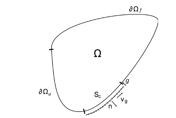
A linear visco-elastic continuous medium with small perturbation hypothesis is considered and the frictional contact interface (with potential phenomena of contact, no-contact, sliding and sticking states) is the only non-linearity considered in the system. This mechanical system can be defined in a domain $\mathsf{\Omega }$ with boundary $\partial \mathsf{\Omega }$ admitting $\left\{\partial {\mathsf{\Omega }}_u,\partial {\mathsf{\Omega }}_f,S_c\right\}$ as partition, and subjected to a surface load ${\mathbf{f}}_{\mathbf{s}}$ and a volume load ${\mathbf{f}}_{\mathbf{v}}$, as illustrated in Figure 2. $\partial {\mathsf{\Omega }}_u$ defines the part of $\partial \mathsf{\Omega }$ where displacement ${\mathbf{u}}_{\mathbf{d}}$ is prescribed, $\partial {\mathsf{\Omega }}_f$ defines the part of $\partial \mathsf{\Omega }$ where surface load is applied and $S_c$ is the potential contact interface with initial gap g. The displacement field $\mathbf{u}$ must verify the local formulations of contact equations, as well as the constitutive relations of continuum mechanics. Using the principle of virtual power, the dynamics of the mechanical system with contact laws can be given by:

$$\left\{\begin{array}{c}\mathrm{find}\mathbf{u}\in \mathcal{U}\mathrm{and}\mathbf{r}\mathrm{such}\mathrm{as}\forall {\dot{\mathbf{u}}}^{🟉}\in {\mathcal{U}}^0\hfill \\ {\displaystyle {\int }_{\mathsf{\Omega }}\rho {\dot{\mathbf{u}}}^{🟉}\ddot{\mathbf{u}}\mathrm{d}\mathsf{\Omega }+{\int }_{\mathsf{\Omega }}{\dot{\epsilon }}^{🟉}\left(\mathcal{B}\dot{\epsilon }+\mathcal{A}\epsilon \right)\mathrm{d}\mathsf{\Omega }={\int }_{\partial {\mathsf{\Omega }}_f}{\dot{\mathbf{u}}}^{🟉}·{\mathbf{f}}_{\mathbf{s}}\mathrm{d}S+{\int }_{\mathsf{\Omega }}{\dot{\mathbf{u}}}^{🟉}·{\mathbf{f}}_{\mathbf{v}}\mathrm{d}\mathsf{\Omega }+{\int }_{S_c}{\dot{\mathbf{u}}}^{🟉}·\mathbf{r}\mathrm{d}S}\hfill \\ {\displaystyle {\int }_{S_c}{r}_n^{🟉}{r}_{n}dS={\int }_{S_c}{r}_n^{🟉}{proj}_{{\mathbb{R}}^{-}}\left(r_n-{\rho }_n^u\left(u_n-g\right)\right)dS}\hfill \\ {\displaystyle {\int }_{S_c}{\mathbf{r}}_{\mathbf{t}}^{🟉}{\mathbf{r}}_{\mathbf{t}}dS={\int }_{S_c}{\mathbf{r}}_{\mathbf{t}}^{🟉}{proj}_{K_{\mu }}\left(\mathbf{r}-{\rho }_t\left(\dot{{\mathbf{u}}_{\mathbf{t}}}-{\mathbf{v}}_{\mathbf{g}}\right)\right)dS}\hfill \end{array}\right.$$

(5)

where $\mathcal{U}=\left\{\mathbf{u},\mathbf{u}={\mathbf{u}}_{\mathbf{d}}\mathrm{on}\partial {\mathsf{\Omega }}_u\right\}$ and ${\mathcal{U}}^0=\left\{\mathbf{u},\mathbf{u}=0\mathrm{on}\partial {\mathsf{\Omega }}_u\right\}$. $\mathcal{B}$ and $\mathcal{A}$ are respectively the viscous stress tensor and the elastic stress tensor. $\epsilon$ and ${\epsilon }^{🟉}$ are the symmetric gradients of $\mathbf{u}$ and ${\mathbf{u}}^{🟉}$, respectively. It can be noted that the two last relations of Equation (5) are equivalent to the fact that $\left(\mathbf{u},\mathbf{r}\right)$ and $\left(\dot{\mathbf{u}},\mathbf{r}\right)$ verify Equations (1) and (2), respectively. This weak formulation of non-smooth frictional contact equations can be found in different forms in the literature [17,18,19,20,21].

It can be observed that any linear law could be considered in the previous modeling. The sliding speed is taken to be an Eulerian sliding speed in order to simplify modeling by considering the fixed configuration of the bodies. In other words, it only appears in the friction equation by modifying the relative speed between the bodies.

2.3. Quasi-Static Solution and Stability Analysis of the Mechanical System with a Frictional Interface

Let’s consider that the boundary conditions are constant in time. The previous dynamic problem defined in Equation (5) has a quasi static solution. This quasi static solution denoted by $\left({\mathbf{u}}^{\mathrm{e}},{\mathbf{r}}^{\mathrm{e}}\right)$ verifies [9]:

$$\left\{\begin{array}{c}{\displaystyle {\int }_{\mathsf{\Omega }}{\dot{\epsilon }}^{🟉}\mathcal{A}{\epsilon }^{\mathrm{e}}\mathrm{d}\mathsf{\Omega }={\int }_{\partial {\mathsf{\Omega }}_f}{\dot{\mathbf{u}}}^{🟉}·{\mathbf{f}}_{\mathbf{s}}\mathrm{d}S+{\int }_{\mathsf{\Omega }}{\dot{\mathbf{u}}}^{🟉}·{\mathbf{f}}_{\mathbf{v}}\mathrm{d}\mathsf{\Omega }+{\int }_{S_c}{\dot{\mathbf{u}}}^{🟉}·{\mathbf{r}}^{\mathrm{e}}\mathrm{d}S,\forall {\dot{\mathbf{u}}}^{🟉}\in U^0}\hfill \\ u_n^{\mathrm{e}}\le 0\mathrm{on}{S}_c\hfill \\ r_n^{\mathrm{e}}\le 0\mathrm{on}{S}_c\hfill \\ {\displaystyle {\mathbf{r}}_{\mathbf{t}}^{\mathrm{e}}=-\mu r_n^{\mathrm{e}}\frac{{\mathbf{v}}_{\mathbf{g}}}{\parallel {\mathbf{v}}_{\mathbf{g}}\parallel }=-\mu r_n^{\mathrm{e}}\mathbf{t}\mathrm{on}{S}_c}\hfill \\ u_n^{\mathrm{e}}{r}_n^{\mathrm{e}}=0\mathrm{on}{S}_c\hfill \end{array}\right.$$

(6)

where ${\epsilon }^{\mathrm{e}}$ and ${\epsilon }^{🟉}$ are the symmetric gradients of ${\mathbf{u}}^{\mathrm{e}}$ and ${\mathbf{u}}^{🟉}$. $(\mathbf{n},\mathbf{t},\mathbf{b})$ defines the local basis on the contact zone, with $\mathbf{t}$ is the sliding direction (i.e., $\mathbf{t}=\frac{{\mathbf{v}}_{\mathbf{g}}}{\parallel {\mathbf{v}}_{\mathbf{g}}\parallel }$), $\mathbf{n}$ being the outward normal and $\mathbf{b}=\mathbf{n}\wedge \mathbf{t}$.

Additionally, a stability analysis of the estimated quasi-static solution has to be investigated. To perform such analysis, a linearization of the the nonlinear equations around this equilibrium point has to be done by considering a perturbation of the solution such as $\left(\mathbf{u},\mathbf{r}\right)=\left({\mathbf{u}}^{\mathrm{e}}+\widehat{\mathbf{u}},{\mathbf{r}}^{\mathrm{e}}+\widehat{\mathbf{r}}\right)$ where the subscript $\widehat{}$ represents the perturbation. It can be noted that this perturbation assumes a strong restriction such that the contact state is unchanged when one goes from the quasi-static solution $\left({\mathbf{u}}^{\mathrm{e}},{\mathbf{r}}^{\mathrm{e}}\right)$ to the disturbed solution around the equilibrium point $\left({\mathbf{u}}^{\mathrm{e}}+\widehat{\mathbf{u}},{\mathbf{r}}^{\mathrm{e}}+\widehat{\mathbf{r}}\right)$.

Thereby the solution $(\widehat{\mathbf{u}},\widehat{\mathbf{r}})$ verifies the following equation:

$$\left\{\begin{array}{c}\mathrm{find}\widehat{\mathbf{u}}\in \mathcal{U}\mathrm{and},\widehat{\mathbf{r}}\mathrm{such}\mathrm{as}\forall {\dot{\mathbf{u}}}^{🟉}\in {\mathcal{U}}^0\hfill \\ {\displaystyle {\int }_{\mathsf{\Omega }}{\dot{\mathbf{u}}}^{🟉}\rho \ddot{\widehat{\mathbf{u}}}\mathrm{d}\mathsf{\Omega }+{\int }_{\mathsf{\Omega }}{\dot{\epsilon }}^{🟉}\left(\mathcal{B}\dot{\widehat{\epsilon }}+\mathcal{A}\widehat{\epsilon }\right)\mathrm{d}\mathsf{\Omega }={\int }_{S_c^{\mathrm{e}}}{\dot{\mathbf{u}}}^{🟉}·\widehat{\mathbf{r}}\mathrm{d}S}\hfill \\ {\widehat{u}}_n=0\mathrm{on}{S}_c^{\mathrm{e}}\hfill \\ {\displaystyle \widehat{{\mathbf{r}}_{\mathbf{t}}}=\mu \left(\frac{r_n^{\mathrm{e}}}{\parallel {\mathbf{v}}_{\mathbf{g}}\parallel }\widehat{\dot{u_b}}\mathbf{b}-\widehat{r_n}\mathbf{t}\right)\mathrm{on}{S}_c^{\mathrm{e}}}\hfill \end{array}\right.$$

(7)

where $\widehat{\epsilon }$ and ${\epsilon }^{🟉}$ are the symmetric gradients of $\widehat{\mathbf{u}}$ and ${\mathbf{u}}^{🟉}$.

Considering that a harmonic solution of Equation (7) is sought of the following form:

$$(\widehat{\mathbf{u}},\widehat{\mathbf{r}})=e^{\lambda t}(\widehat{{\mathbf{u}}_0},\widehat{{\mathbf{r}}_0})$$

(8)

the previous variational Equation (7) can be rewritten as follows:

$$\left\{\begin{array}{c}\mathrm{find}{\widehat{\mathbf{u}}}_{\mathbf{0}}\in \mathcal{U},\widehat{{\mathbf{r}}_0}\mathrm{and}\lambda \in \mathbb{C}\mathrm{such}\mathrm{as}\forall {\dot{\mathbf{u}}}^{🟉}\in {\mathcal{U}}^0\hfill \\ {\lambda }^2\mathcal{M}\left({\widehat{\mathbf{u}}}_{\mathbf{0}},{\dot{\mathbf{u}}}^{🟉}\right)+\lambda \widehat{\mathcal{C}}\left({\widehat{\mathbf{u}}}_{\mathbf{0}},{\dot{\mathbf{u}}}^{🟉}\right)+\mathcal{K}\left({\widehat{\mathbf{u}}}_{\mathbf{0}},{\dot{\mathbf{u}}}^{🟉}\right)={\int }_{S_c^{\mathrm{e}}}{\widehat{\mathbf{r}}}_{\mathbf{0}\mathbf{n}}{\dot{\mathbf{u}}}^{🟉}·\left(\mathbf{n}-\mu \mathbf{t}\right)\mathrm{d}S\hfill \\ {\widehat{\mathbf{u}}}_{\mathbf{0}}·\mathbf{n}=0\mathrm{on}{S}_c^{\mathrm{e}}\hfill \end{array}\right.$$

(9)

with

$$\widehat{\mathcal{C}}\left({\widehat{\mathbf{u}}}_{\mathbf{0}},{\mathbf{u}}^{🟉}\right)=\mathcal{C}\left({\widehat{\mathbf{u}}}_{\mathbf{0}},{\mathbf{u}}^{🟉}\right)-{\int }_{S_c^{\mathrm{e}}}\mu \frac{r_n^{\mathrm{e}}}{\parallel {\mathbf{v}}_{\mathbf{g}}\parallel }{\widehat{u_0}}_b{u}_b^{🟉}\mathrm{d}S$$

(10)

$\mathcal{M}$, $\mathcal{C}$ and $\mathcal{K}$ are respectively the mass, damping and stiffness operators of the structure without contact. It can be noted that the damping operator $\widehat{\mathcal{C}}$ is composed of the damping operator of the structure without contact (i.e., $\mathcal{C}$) plus an additional contribution due to the linearization of the sliding direction for $3D$-cases that gives the term along $\mathbf{b}$ in Equation (7). The last relation in Equation (9) (i.e., ${\widehat{\mathbf{u}}}_{\mathbf{0}}·\mathbf{n}=0$) can be imposed by searching ${\widehat{\mathbf{u}}}_{\mathbf{0}}$ in ${\mathcal{W}}^0$ whereas contact forces may be eliminated by searching ${\dot{\mathbf{u}}}^{🟉}$ in ${\mathcal{W}}^{\mu }$ leading to a non symmetric complex eigenvalue problem:

$$\left\{\begin{array}{c}\mathrm{find}{\widehat{\mathbf{u}}}_{\mathbf{0}}\in {\mathcal{W}}_0\mathrm{and},\lambda \in \mathbb{C}\mathrm{such}\mathrm{that}\forall {\dot{\mathbf{u}}}^{🟉}\in {\mathcal{W}}^{\mu }\hfill \\ {\lambda }^2\mathcal{M}\left({\widehat{\mathbf{u}}}_{\mathbf{0}},{\dot{\mathbf{u}}}^{🟉}\right)+\lambda \widehat{\mathcal{C}}\left({\widehat{\mathbf{u}}}_{\mathbf{0}},{\dot{\mathbf{u}}}^{🟉}\right)+\mathcal{K}\left({\widehat{\mathbf{u}}}_{\mathbf{0}},{\dot{\mathbf{u}}}^{🟉}\right)=0\hfill \end{array}\right.$$

(11)

where ${\mathcal{W}}^0=\left\{\mathbf{u},\mathbf{u}·\mathbf{n}=0\mathrm{on}{S}_c^{\mathrm{e}}\right\}$ and ${\mathcal{W}}^{\mu }=\left\{\mathbf{u},\mathbf{u}·\left(\mathbf{n}-\mu \mathbf{t}\right)=0\mathrm{on}{S}_c^{\mathrm{e}}\right\}$.

3. Finite Element Formulation and Solving

3.1. Finite Element Discretization of the Nonlinear Dynamics Problem

Using classical finite element discretization of the problem, the nonlinear dynamics problem given in Equation (5) can be rewritten as follows:

$$\mathbf{M}\ddot{\mathbf{u}}+\mathbf{C}\dot{\mathbf{u}}+\mathbf{K}\mathbf{u}=\mathbf{f}+{\mathbf{r}}_{\mathbf{c}}$$

(12)

where $\mathbf{M}$, $\mathbf{K}$ and $\mathbf{C}$ are the classical mass, stiffness and damping matrices of the mechanical system. $\mathbf{f}$ and ${\mathbf{r}}_{\mathbf{c}}$ are the generalized force and the contact reactions respectively.

By making explicit the different contributions of the contact reactions in more details, the following form can be given:

$$\mathbf{M}\ddot{\mathbf{u}}+\left(\mathbf{C}-\mu {{\mathbf{P}}_{\mathbf{b}}}^T\mathbf{D}{\mathbf{P}}_{\mathbf{b}}\right)\dot{\mathbf{u}}+\mathbf{K}\mathbf{u}=\mathbf{f}+{{\mathbf{P}}_{\mathbf{n}}}^T{\mathbf{R}}_{\mathbf{n}}+{{\mathbf{P}}_{\mathbf{t}}}^T{\mathbf{R}}_{\mathbf{t}}$$

(13)

where ${\mathbf{R}}_{\mathbf{n}}$ and ${\mathbf{R}}_{\mathbf{t}}$ define the vectors of normal reactions and friction forces at the contact interfaces. ${\mathbf{P}}_{\mathbf{n}}$, ${\mathbf{P}}_{\mathbf{t}}$ and ${\mathbf{P}}_{\mathbf{b}}$ are the projection matrices on the normal, the first and second tangential directions at contact nodes. In other words these matrices allow to pass the contact reactions from the local relative frame to the global frame of the problem. The matrix $\mathbf{D}$ is defined by $D_{ii}=\frac{{\left(r_n^{\mathrm{e}}\right)}_i}{{\left(v_g\right)}_i}$ with ${\left(v_g\right)}_i$ is the norm of the sliding speed ${\mathbf{v}}_{\mathbf{g}}$ at the ith node. Considering more specifically the contact laws, several discretization methods exist based on different interpolation function choices [19]. However, the use of linear interpolation functions for forces and contact displacements allows contact Equations (3) and (4) to be considered at each mesh node using equivalent reaction forces [21]:

$${\mathbf{R}}_{\mathbf{n}}={proj}_{{\mathbb{R}}^{-}}\left({\mathbf{R}}_{\mathbf{n}}-{\rho }_{\mathbf{n}}{\mathbf{G}}_{\mathbf{n}}\right),\forall {\rho }_{\mathbf{n}}\mathrm{such}\mathrm{as}{\rho }_{\mathbf{n}},ii>0\mathrm{and}{\rho }_{\mathbf{n}},i\ne j=0$$

(14)

$$\left\{\begin{array}{c}{\mathbf{R}}_{\mathbf{t}}\hfill \\ {\mathbf{R}}_{\mathbf{b}}\hfill \end{array}\right\}={proj}_{K_{\mu }}\left(\left\{\begin{array}{c}{\mathbf{R}}_{\mathbf{t}}\hfill \\ {\mathbf{R}}_{\mathbf{b}}\hfill \end{array}\right\}-{\rho }_{\mathbf{t}}\left\{\begin{array}{c}\dot{{\mathbf{G}}_{\mathbf{t}}}-{\mathbf{v}}_{\mathbf{g}}\\ \dot{{\mathbf{G}}_{\mathbf{b}}}\end{array}\right\}\right),\forall {\rho }_{\mathbf{t}}\mathrm{such}\mathrm{as}{\rho }_{\mathbf{t}},ii>0\mathrm{and}{\rho }_{\mathbf{t}},i\ne j=0$$

(15)

where ${\rho }_{\mathbf{n}}$ and ${\rho }_{\mathbf{t}}$ are two diagonal matrices composed of positive real numbers that correspond to the normal and tangential augmentation parameters, respectively.

3.2. Stability Analysis

As a reminder the linearized equations of motion are obtained by introducing small perturbations about the quasi-static equilibrium. It leads to linearized contact laws (see Equations (7)) given by:

$$\left\{\begin{array}{c}{u}_n=0\hfill \\ {\displaystyle {\mathbf{r}}_{\mathbf{t}}=\mu \left(\frac{r_n^{\mathrm{e}}}{\parallel {\mathbf{v}}_{\mathbf{g}}\parallel }\dot{u_b}\mathbf{b}-r_n\mathbf{t}\right)}\hfill \end{array}\right.$$

(16)

Considering the previous formulation (12), the quasi-static equilibrium ${\mathbf{u}}^{\mathbf{e}}$ is estimated by using the following relation:

$$\mathbf{K}{\mathbf{u}}^{\mathbf{e}}=\mathbf{f}+{{\mathbf{P}}_{\mathbf{n}}}^T{\mathbf{R}}_{\mathbf{n}}^{\mathbf{e}}+{{\mathbf{P}}_{\mathbf{t}}}^T{\mathbf{R}}_{\mathbf{t}}^{\mathbf{e}}$$

(17)

where ${\mathbf{R}}_{\mathbf{n}}^{\mathbf{e}}$ and ${\mathbf{R}}_{\mathbf{t}}^{\mathbf{e}}$ are the generalized contact reactions that verify Equations (3) and (4) at each mesh node for the discretized displacement ${\mathbf{u}}^{\mathbf{e}}$. The relation (17) corresponds to the previous formulation of the quasi-static solution in continuum mechanics given in Equation (6).

Finally, the stability analysis can be investigated by considering the following eigenvalue problem to be solved:

$$\left({\lambda }^2\tilde{\mathbf{M}}+\lambda \tilde{\mathbf{C}}+\tilde{\mathbf{K}}\right)\tilde{\mathbf{u}}=\mathbf{0}$$

(18)

where $\tilde{\mathbf{u}}$ defines the vector of a small perturbation around the previous estimated sliding equilibrium ${\mathbf{u}}^{\mathbf{e}}$. $\tilde{\mathbf{M}}$, $\tilde{\mathbf{C}}$ and $\tilde{\mathbf{K}}$ are the nonsymmetric mass, damping and stiffness matrices given by:

$$\tilde{\mathbf{M}}={\mathbf{T}}_{\mu }^T\mathbf{M}{\mathbf{T}}_{\mathbf{n}}$$

(19)

$$\tilde{\mathbf{K}}={\mathbf{T}}_{\mu }^T\mathbf{K}{\mathbf{T}}_{\mathbf{n}}$$

(20)

$$\tilde{\mathbf{C}}={\mathbf{T}}_{\mu }^T\left(\mathbf{C}-\mu {{\mathbf{P}}_{\mathbf{b}}}^T\mathbf{D}{\mathbf{P}}_{\mathbf{b}}\right){\mathbf{T}}_{\mathbf{n}}$$

(21)

where ${\mathbf{T}}_{\mathbf{n}}$ defines the basis of the fields orthogonal to the normal $\mathbf{n}$ to the equilibrium contact interfaces (i.e., the basis of the finite element approximated ${\mathcal{W}}^0$) and ${\mathbf{T}}_{\mu }$ defines the basis of the fields orthogonal to the direction $\mathbf{n}-\mu \mathbf{t}$ on the equilibrium contact interfaces (i.e., the basis of the finite element approximated ${\mathcal{W}}^{\mu }$). Solving such a problem can be achieved by using the Residual Iteration Method [22].

Then the local stability of the quasi-static equilibrium ${\mathbf{u}}^{\mathbf{e}}$ can be studied by examining the complex eigenvalues $\lambda$. The mechanical system is unstable if at least one eigenvalues has a real part superior to zero. On the other hand, the system is stable if all the real parts of eigenvalues are negative. The imaginary part of eigenvalues defines the frequencies of each mode.

3.3. Transient Non-Linear Temporal Response and Integration Scheme

In addition to the estimation of the stability of the system (i.e., the estimation of the equilibrium points and the stability of the latter), it is necessary to estimate the temporal vibrational response of the system if the latter is unstable. In order to be able to deal with non-smooth contact dynamics problem a first order modified $\theta$-method time integration scheme [14,23] (with $\theta =0.5$) is used with a time step $\tau$. The choice of the value of $\theta$ is essential in order to avoid numerical damping for liner problems and therefore to avoid introducing errors in the estimation of the dynamic solution of the problem. Moreover this integration scheme is unconditionally stable for $\theta =0.5$ [23,24]. This integration scheme was previously used for example in the following works [25,26,27,28,29].

The time discretized equations governing the nonlinear system between two time steps $t^i$ and $t^{i+1}$ is given by [9]:

$$\left\{\begin{array}{c}{\displaystyle \mathbf{M}\left({\dot{\mathbf{u}}}^{i+1}-{\dot{\mathbf{u}}}^i\right)=\tau \theta \left({\mathbf{f}}^{i+1}-\mathbf{K}{\mathbf{u}}^{i+1}-\mathbf{C}{\dot{\mathbf{u}}}^{i+1}\right)+\tau \left(1-\theta \right)\left({\mathbf{f}}^i-\mathbf{K}{\mathbf{u}}^i-\mathbf{C}{\dot{\mathbf{u}}}^i\right)+\tau {\mathbf{r}}_{\mathbf{c}}^{i+1}}\hfill \\ {\displaystyle {\mathbf{u}}^{i+1}={\mathbf{u}}^i+\tau \left(\theta {\dot{\mathbf{u}}}^{i+1}+\left(1-\theta \right){\dot{\mathbf{u}}}^i\right)}\hfill \end{array}\right.$$

(22)

with $\left(\mathbf{u},\dot{\mathbf{u}},{\mathbf{r}}_{\mathbf{c}}\right)$ verifying Equations (3) and (4) at each mesh node. It is important to note that, when dealing with shocks between two elastic bodies, any other value than $\theta =1$ is unable to guarantee the inelastic shock. One way to overcome this huge problem is to evaluate the relative displacement for the computation of the contact reactions as follows:

$${\tilde{\mathbf{u}}}^{i+1}={\mathbf{u}}^{i+1}+\tau \left(1-\theta \right){\dot{\mathbf{u}}}^{i+1}$$

(23)

this procedure is called the modified $\theta$-method. It introduces a bias: the new estimation of the displacement ${\tilde{\mathbf{u}}}^{i+1}$ introduces a contact reaction before the shock occurs. However this allows to impose a contact reaction such that the shock occurs exactly on a time step. By taking this relation (23) in the formulation of the frictional contact laws given by Equations (3) and (4), the two following expressions can be obtained:

$${{\mathbf{R}}_{\mathbf{n}}}^{i+1}={proj}_{{\mathbb{R}}^{-}}\left({{\mathbf{R}}_{\mathbf{n}}}^{i+1}-{\rho }_{\mathbf{n}}\left({\dot{{\mathbf{G}}_{\mathbf{n}}}}^{i+1}+\left(1-\theta \right){\dot{{\mathbf{G}}_{\mathbf{n}}}}^i+\frac{{{\mathbf{G}}_{\mathbf{n}}}^i}{\tau }\right)\right),\forall {\rho }_{\mathbf{n}}\mathrm{diagonal}\mathrm{and}\mathrm{positive}$$

(24)

$$\left\{\begin{array}{c}{{\mathbf{R}}_{\mathbf{t}}}^{i+1}\hfill \\ {{\mathbf{R}}_{\mathbf{b}}}^{i+1}\hfill \end{array}\right\}={proj}_{K_{\mu }}\left(\left\{\begin{array}{c}{{\mathbf{R}}_{\mathbf{t}}}^{i+1}\hfill \\ {{\mathbf{R}}_{\mathbf{b}}}^{i+1}\hfill \end{array}\right\}-{\rho }_{\mathbf{t}}\left\{\begin{array}{c}{\dot{{\mathbf{G}}_{\mathbf{t}}}}^{i+1}-{\mathbf{v}}_{\mathbf{g}}\\ {\dot{{\mathbf{G}}_{\mathbf{b}}}}^{i+1}\end{array}\right\}\right),\forall {\rho }_{\mathbf{t}}\mathrm{diagonal}\mathrm{and}\mathrm{positive}$$

(25)

An iterative fixed point algorithm on equivalent contact reactions and friction forces with a stop criterion based on forces convergence [9,18] can be used for the computation of the quasi-static solution and dynamics solutions at each time step. This algorithm is appropriate to the formulation of the frictional contact laws as nonlinear projections (24) and (25). The main advantage of the fixed point algorithm lies on the fact that the integrator matrix remains constant at each iteration.

4. Numerical Example

Previous numerical studies for finite element mechanical systems subjected to friction-induced vibrations have been performed by using the non smooth contact dynamics approach [7,8,9,10,13].

The objective of the following numerical results is to provide an illustration and discussion on the use of non smooth contact formulation in the context of brake squeal, and to highlight the potential links between the self-excited vibration of the complete brake system and the contact dynamics at the frictional interfaces.

4.1. Finite Element Model of the Brake System under Study

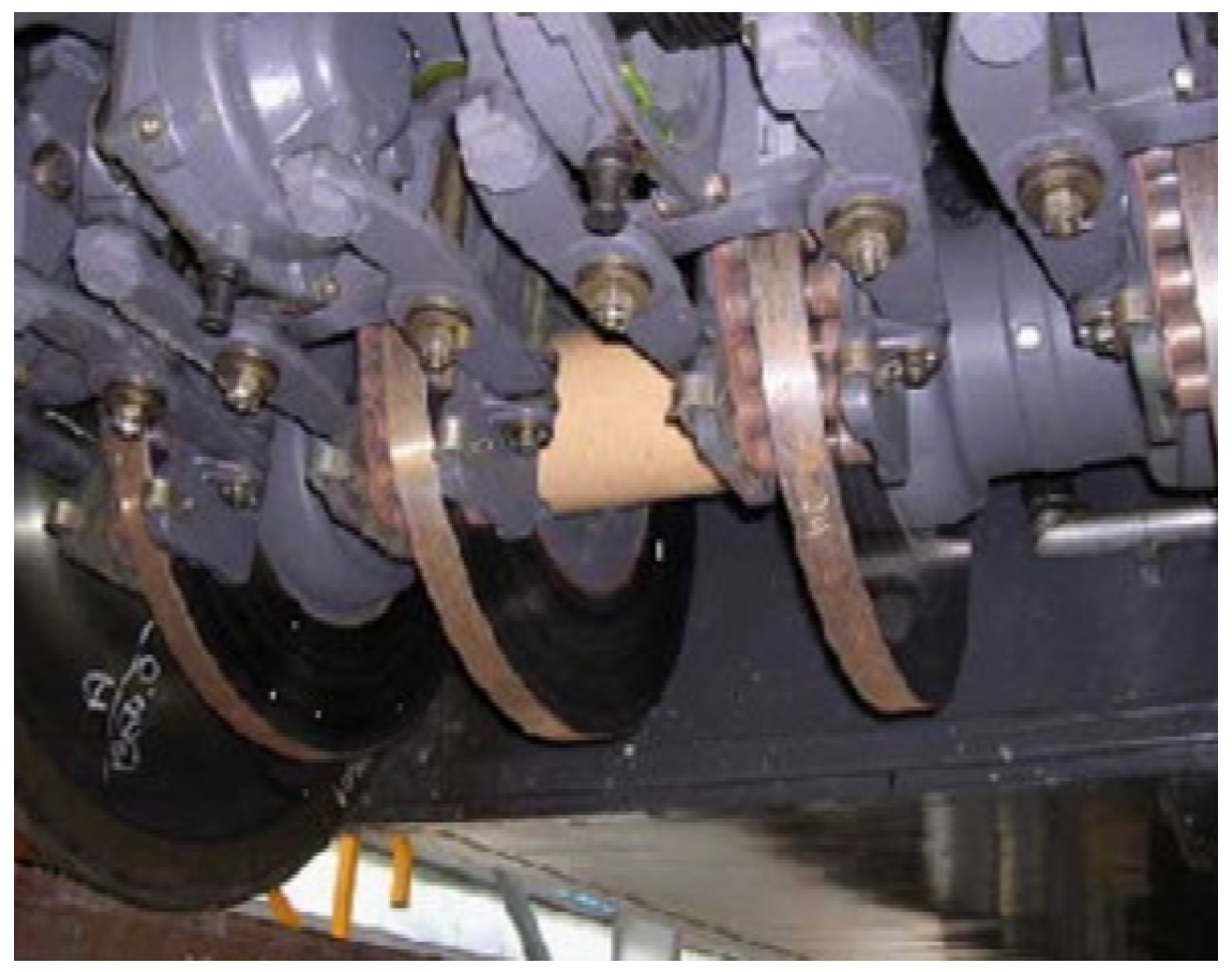
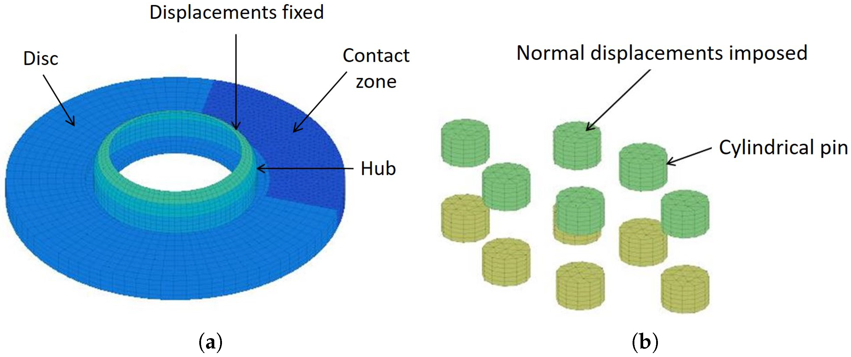
The finite element model under study aims to study instabilities of the TGV (French high-speed train) braking system. A picture of such a braking system is given in Figure 3. Figure 4 illustrates the associated finite element model under study. It corresponds to a simplified brake system that is composed of one disc and a set of 6 small cylindrical pins applied on either sides of the disc. This finite element model has:

• 27,090 degrees-of-freedom for the bell/disc system;
• 4884 degrees-of-freedom for all the lining;
• 1368 degrees of freedom at the frictional contact zone between the disc and the 12 small cylindrical pins.

The different boundary conditions of the problem are indicated in Figure 4. The material and geometrical properties of the system are given in

Table 1. Material and geometrical properties of the brake system.

Parameter	Variable	Value
Rayleigh damping for hub and disc—mass contribution	${\alpha }_{disc}$	$7.50$ s${}^{-1}$
Rayleigh damping for hub and disc—stiffness contribution	${\beta }_{disc}$	$1.0\times {10}^{-7}$ s
Rayleigh damping for pads and backplate—mass contribution	${\alpha }_{gar}$	135 s${}^{-1}$
Rayleigh damping for pads and backplate—stiffness contribution	${\beta }_{gar}$	$1.80\times {10}^{-6}$ s
Normal force applied on the caliper support	$F_{ext}$	2000 N
Young modulus for hub and disc	$E_{\mathrm{disc}}$	210 GPa
Mass density for hub and disc	${\rho }_{\mathrm{disc}}$	7850 kg/m${}^3$
Poisson coefficient for hub and disc	${\nu }_{\mathrm{disc}}$	$0.28$
Young modulus for pads	$E_{\mathrm{pad}}$	$2.0$ GPa
Mass density for pads	${\rho }_{\mathrm{pad}}$	5000 kg/m${}^3$
Poisson coefficient for pads	${\nu }_{\mathrm{pad}}$	$0.3$
Normal displacement imposed on the outer face of the pins	$U_{pin}^{imposed}$	$1.60\times {10}^{-6}$ m

.

In the following the coupling modes due to friction forces is considered as the main cause of squeal. For the interested reader, it can be noted that the tribological or thermal effects that can be invoked in order to better explain the occurrence of instability are neglected.

4.2. Stability Analysis

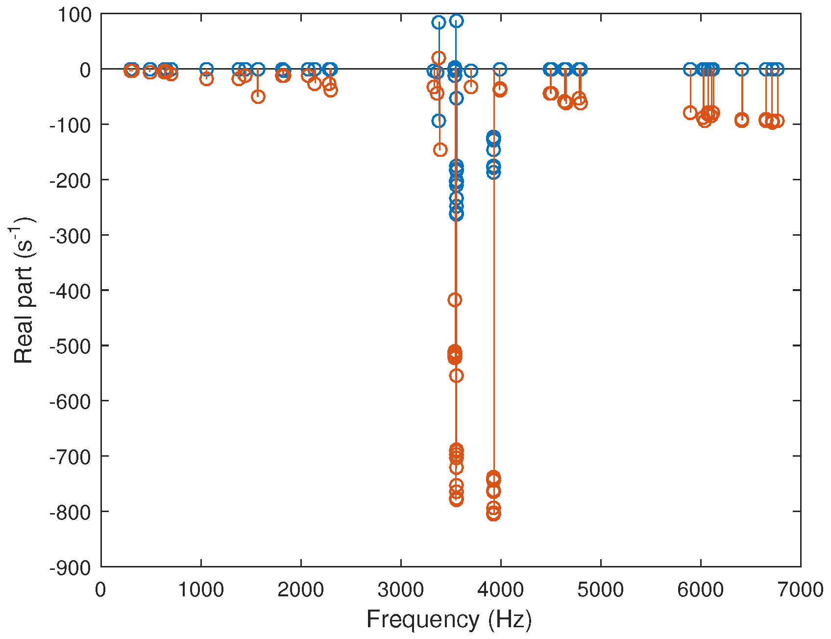
Stability analysis is conducted by applying the process previously proposed in Section 3.2. Figure 5 gives a typical result of the stability chart for $\mu =0.2$. Two cases are illustrated: the first one corresponds to the brake system with Rayleigh damping and the second one corresponds to the brake system without Rayleigh damping. In the first case, two unstable modes are detected, while in the second case only one unstable mode remains, the second unstable mode having disappeared due to the addition of Rayleigh damping. In the case of the system without Rayleigh damping, a notable damping effect is also visible for the modes around [3000;4000] Hz, which illustrates the role of the additional damping contribution due to the friction at disc/pin interfaces. 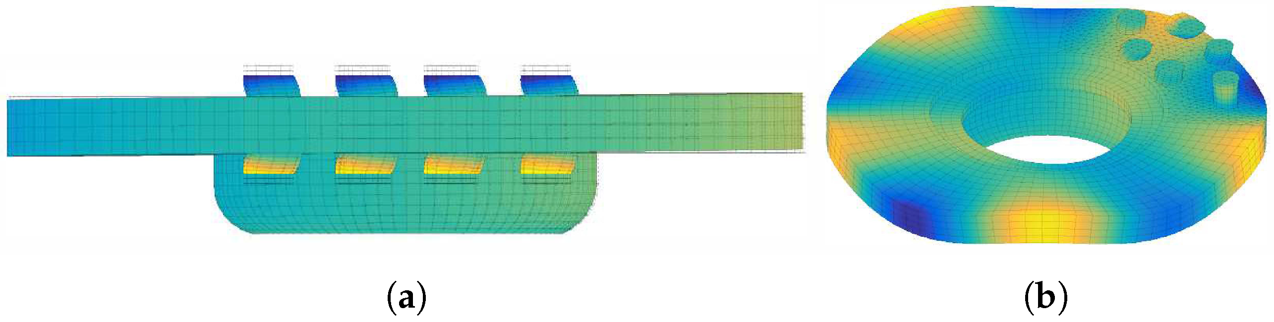Figure 6 illustrate the quasi-static sliding equilibrium of the brake system and the unstable mode shape for the case with Rayleigh damping. The effects of the braking force and the friction reactions between the rotating disc and the pins are clearly visible on the equilibrium position. It should also be observed that the unstable mode is composed of a shape deformation of both the disc and the pins. 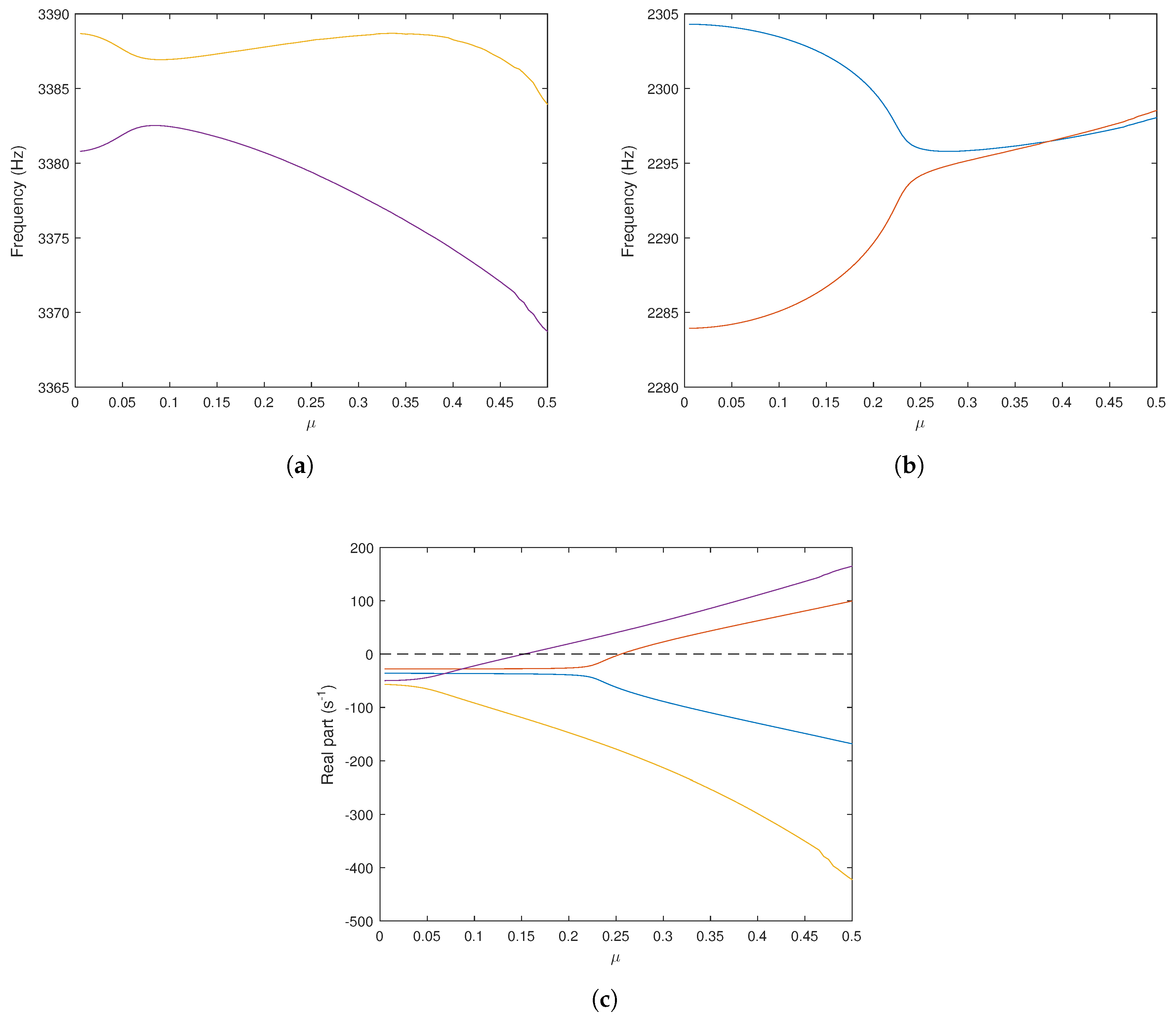Figure 7 give the evolutions of the two coupling modes versus the friction coefficient (for $\mu =[0;0.5]$), as well as the evolution of the associated real parts. It is observed that the brake system is stable for a friction coefficient $\mu$ inferior to 0.16. For $0.16<\mu <0.26$ one instability is detected. The frequency of this unstable mode is around [3380;3365] Hz depending on the value of the coefficient of friction. For $\mu >0.26$, two mode coupling are present with the appearance of a second unstable mode around [2294;2298] Hz. For each instability, the coalescence pattern is not perfect due to the Rayleigh damping (for more details on the role of damping, see [11]).

4.3. Nonlinear Simulation

The configuration with $\mu =0.2$ is chosen to estimate the nonlinear solution of the problem and the self-excited vibrations. All the results are estimated by applying the previous process based on the modified $\theta$-method, as discussed in Section 3.3.

4.3.1. Friction-Induced Steady State Vibrations

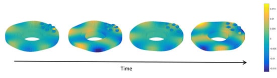
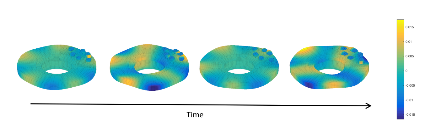
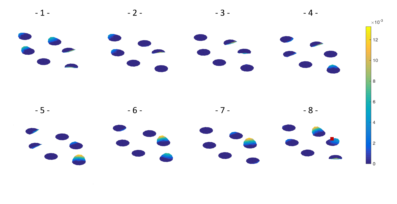
Figure 8 illustrates the evolution of the self-sustained steady state vibration of the brake system over one period. The disc and the cylindrical pins vibrate with maximum amplitudes of 0.015 m. Figure 9 shows the evolution the upper contact zones between the disc and the cylindrical pins. It is clearly observed strongly nonlinear events with contact and no contact states for each contact zone. A maximum gap of 0.0012 m between the disc and one pad is generated when non contact states occur.

Then Figure 10 illustrate the displacements and limit cycles according to the tangential, radial and normal directions for one node at one disc/pin interface. The position of this node is marked by a red square at the bottom right in Figure 9. As shown in Figure 10e, one separation (i.e., no contact state) per period is observed. This results in a variation of the normal speed for a relative displacement equal to zero for the associated limit cycle (see Figure 10f). Moreover discontinuities observed on the limit cycle before the impact (i.e., contact state) are due to impact phases on the adjacent nodes to the considered point.

Finally it is important to recall that the initial conditions can affect the transient nonlinear response, as well as the final friction-induced steady state vibrations. In the case under study it has been verified that various initial conditions always lead to the same final limit cycle solution. This can be explained by the fact that the system has only one unstable mode in the present case and that the influence of the initial conditions on the limit cycles is more generally found for mechanical systems having many unstable modes [9]. Effectively the frequency signature of a system with many unstable modes can be more complex with the presence of the fundamental frequencies, the harmonics contributions, as well as the combinations of fundamental frequency. Thereby the actuation of different frequency contributions during squeal events according to the initial conditions can be more important for such system implying a more important influence of the initial conditions on the nonlinear transient response, as well as the steady state limit cycles.

4.3.2. Evolution of the Mechanical Energy

This section is devoted to the temporal evolution of some specific physical quantities. The evolution of the mechanical energy, the normal force, as well as the status of nodes during the transient ans stationary regimes will be more specifically discussed.

First of all the mechanical energy $E\left(t\right)$ of the brake system is estimated as follows:

$$E=\frac{1}{2}{\mathbf{u}}^T\mathbf{Ku}+\frac{1}{2}{\dot{\mathbf{u}}}^T\mathbf{M}\dot{\mathbf{u}}$$

(26)

and the average mechanical energy $\overline{E}\left(t\right)$ on the chosen time interval $\mathsf{\Delta }T$ is given by:

$${\displaystyle \overline{E}\left(t_j\right)=\frac{1}{n_T}\sum _{k\in {\tau }_j}E\left(t_k\right)}$$

(27)

where $n_T$ is the number of time steps over time $\mathsf{\Delta }T$ and ${\tau }_j$ defines the set of time steps k such as $|t_k-t_j|\le \frac{\mathsf{\Delta }T}{2}$. This average evolution $\overline{E}\left(t_j\right)$ is calculated on sliding time windows of size $\mathsf{\Delta }T=10$ ms with an overlap of 50%, which corresponds to 80 windows for a duration of simulation of 400 ms. Moreover the rate of relative change of the mean mechanical energy ${\overline{\tau }}_E\left(t\right)$ by removing the contribution of the equilibrium point is estimated by using the following relation:

$${\overline{\tau }}_E=\frac{1}{\overline{E}}\overline{\frac{\partial E}{\partial t}}$$

(28)

where $\overline{E}$ and $\overline{\frac{\partial E}{\partial t}}$ are calculated without taking into account the contribution of the equilibrium. The variation of the mechanical energy in time $\frac{\partial E}{\partial t}$ is given by:

$$\frac{\partial E}{\partial t}=\frac{E\left(t_{i+1}\right)-E\left(t_i\right)}{t_{i+1}-t_i}$$

(29)

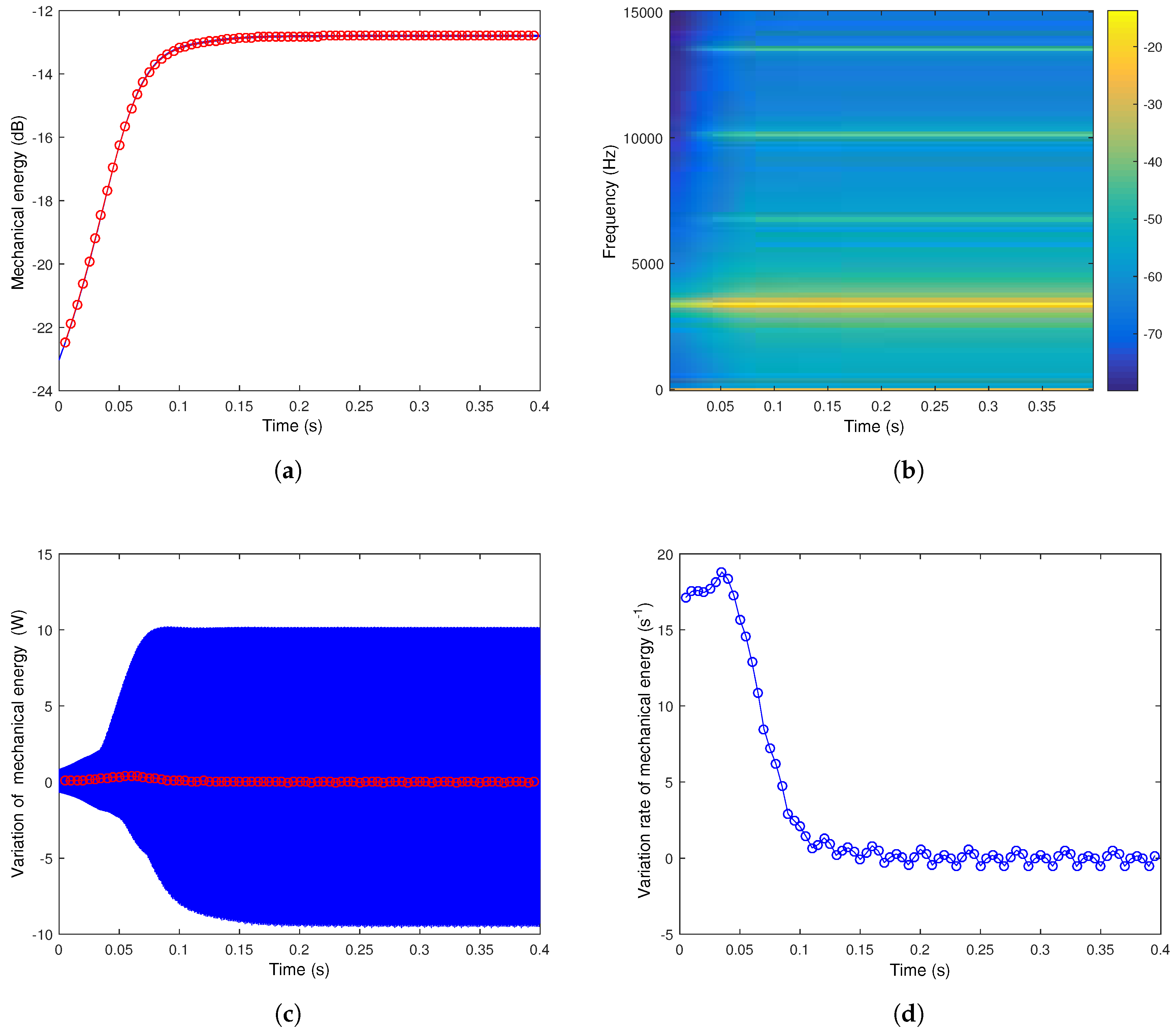
Figure 11a illustrates the evolution of the mechanical energy of the brake system and its associated average mechanical energy. It is clearly observed that the instantaneous mechanical energy $E\left(t\right)$ increases during the transient squeal events with the amplitude growth of oscillations and then stabilizes when the stationary self-sustained vibrations are established. It is observed that the curves of the average mechanical energy $\overline{E}\left(t\right)$ and the instantaneous mechanical energy $E\left(t\right)$ are merged which means that the variation of the mechanical energy $\frac{\partial E}{\partial t}$ is lower than the intrinsic mechanical energy during the squeal events, as also indicated in Figure 11c. Figure 11b also gives the spectrogram of the mechanical energy in dB. The nonlinear squeal events during the transient and stationary regimes are composed of the fundamental frequency of the unstable mode (around 3380 Hz) and the nth associated harmonic components (with $n=1,\dots ,3$ in Figure 11b). This result clearly indicates the potential underestimation effect of the stability analysis which does not make it possible to predict the emergence of the frequencies resulting from a non-linear phenomenon and consequently the presence of the harmonics of the fundamental frequency in this specific case. Finally, Figure 11d illustrates the evolution of the rate of relative change of the mean mechanical energy. A decrease of ${\overline{\tau }}_E$ is first observed until it reaches zero when the established regime is obtained. This demonstrates that the stabilization phenomenon of the squeal event and the detection of the time instant corresponding to the establishment of the limit cycles can be directly estimated from the evolution of ${\overline{\tau }}_E$ and its stabilization around the zero value.

4.3.3. Effective Braking Force over Time

In this section the evolution of the effective braking force $N_b$ is undertaken. Its average evolution is also estimated as follows

$$\overline{N_b}\left(t_j\right)=\frac{1}{n_t}\sum _{k\in {\tau }_j}{N}_b\left(t_k\right)$$

(30)

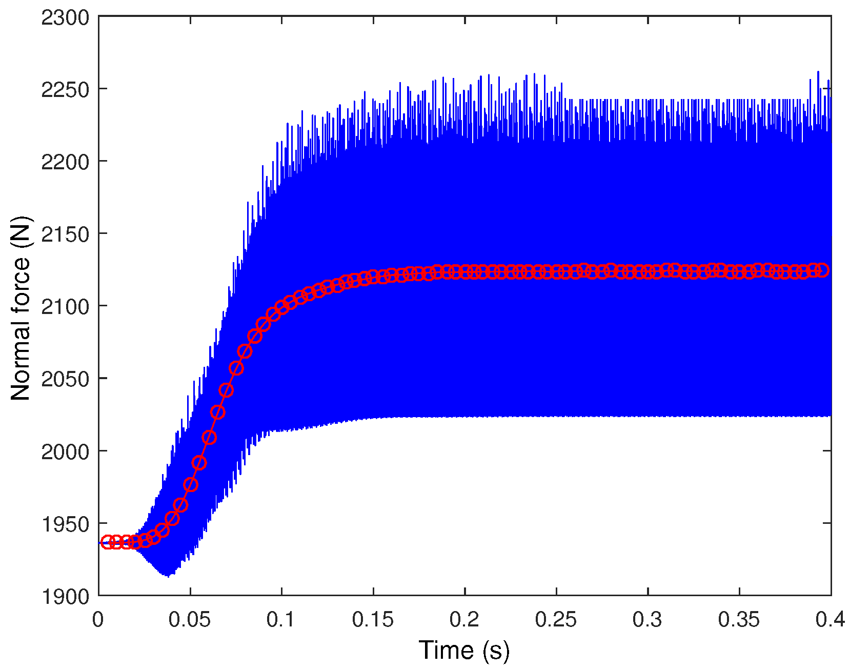
Figure 12 represents the evolution of the effective braking force $N_b$ and its mean $\overline{N_b}$. An increase of $\overline{N_b}$ is observed during the transient squeal event (for t = [0;0.15] s). When the steady state regime is reached, the average mean braking force remains constant (with a value of 2120 N). During this second phase, the instantaneous effective braking force $N_b$ oscillates around this average value with an amplitude of plus or minus 220 N. These oscillations of $N_b$, which do not attenuate in steady state regime, can be explained physically by the non-linear phenomena (i.e., contacts and loss of contacts) at the frictional interfaces between the disc and the 12 cylindrical pins. Finally it is worth noting that this variation of $\overline{N_b}$ during the transient squeal event directly reflects a change in the quasi-static equilibrium of the brake system. In the present case, this evolution of the equilibrium does not change the nonlinear squeal signature.

4.3.4. Node Status at Frictional Interfaces over Time

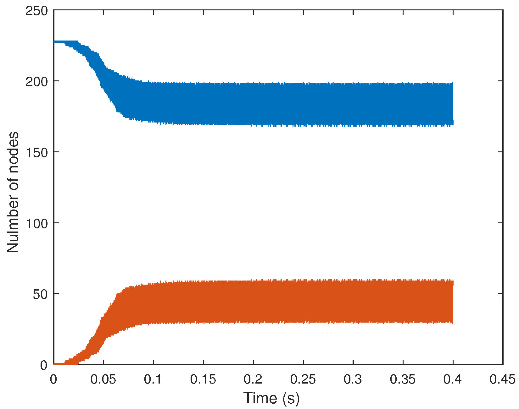
The number of nodes being in sliding contact or separation between disc and pins are given Figure 13. First no sticking phenomenon is observed during the squeal events. This fact can be explained by the value of the rotational speed that imposes a high quasi-static sliding speed at contact nodes, and so excluding a potential sticking phenomenon. It is also observed that the number of interface nodes with no contact state increases gradually during the transient squeal events until it stabilizes for a maximum value of about 60. Once this saturation is reached, the number of interface nodes with no contact state oscillates between 30 and 60. This observation valids the hypothesis that nonlinear phenomena at the frictional interfaces between the disc and all the cylindrical pins are responsible of the energy saturation injected into the contact and lead to the stationary regime.

5. Conclusions

The paper proposed a discussion on the problem of friction-induced vibrations for brake systems with non-smooth contact dynamics. A reminder of the mathematical and theoretical problem is presented as well as the finite element discretization of the nonlinear dynamics problem. The resolution of the nonlinear problem from a numerical point of view is recalled for the determination of the quasi-static equilibrium, its stability analysis, and the prediction of transient and stationary vibrations.

A complete numerical analysis is performed as an illustration of solving a nonlinear dynamics problem with non smooth contact for a finite element brake model. In addition to the determination of the sliding equilibrium point and its stability analysis, special attention was paid to the nonlinear simulation and the calculation of the transient and steady state vibrations. Based on the evolution of the mechanical energy and the node status at contact interfaces over time, it is highlighted that the contact dynamics at each frictional interface is at the origin of the squeal phenomena and its saturation. This numerical example for mechanical system subjected to friction-induced vibration is an interesting illustrated example of the coupling between local (i.e., contact and friction between the disc and the cylindrical pins) and system (i.e., structure scale of the complete brake system) dynamics. As a consequence, the modeling of contact dynamics is a relevant issue in vibrational mechanics for the problem of brake squeal due to the fact that it plays a role of primary importance of both the stability analysis and the prediction of self-excited vibrations.

References

- Crolla, D.A.; Lang, A.M. Brake noise and vibration: State of art. Veh. Tribol. 1991, 18, 165–174. [Google Scholar]
- Kinkaid, N.M.; O’Reilly, O.M.; Papadopoulos, P. Automotive disc brake squeal. J. Sound Vib. 2003, 267, 105–166. [Google Scholar] [CrossRef]
- Ouyang, H.; Nack, W.; Yuan, Y.; Chen, F. Numerical analysis of automotive disc brake squeal: A review. Int. J. Veh. Noise Vib. 2005, 1, 207–231. [Google Scholar] [CrossRef]
- Signorini, A. Questioni di elasticita non linearizzata e semilinearizzata. Rendiconti di Matematica e delle sue Applicazioni 1959, 18, 95–139. [Google Scholar]
- Tonazzi, D.; Massi, F.; Salipante, M.; Baillet, L.; Berthier, Y. Estimation of the normal contact stiffness for frictional interface in sticking and sliding conditions. Lubricants 2019, 7, 56. [Google Scholar] [CrossRef]
- Lorang, X.; Foy-Margiocchi, F.; Nguyen, Q.S.; Gautier, P.E. Tgv disc brake squeal. J. Sound Vib. 2006, 293, 735–746. [Google Scholar] [CrossRef]
- Lorang, X.; Chiello, O. Stability and transient analysis in the modeling of railway disc brake squeal. Notes Numer. Fluid Mech. Multidiscip. Des. 2008, 99, 447–453. [Google Scholar]
- Brizard, D.; Chiello, O.; Sinou, J.-J.; Lorang, X. Performances of some reduced bases for the stability analysis of a disc/pads system in sliding contact. J. Sound Vib. 2011, 330, 703–720. [Google Scholar] [CrossRef]
- Loyer, A.; Sinou, J.-J.; Chiello, O.; Lorang, X. Study of nonlinear behaviors and modal reductions for friction destabilized systems. application to an elastic layer. J. Sound Vib. 2012, 331, 1011–1041. [Google Scholar] [CrossRef][Green Version]
- Sinou, J.-J.; Loyer, A.; Chiello, O.; Mogenier, G.; Lorang, X.; Cocheteux, F.; Bellaj, A. A global strategy based on experiments and simulations for squeal prediction on industrial railway brakes. J. Sound Vib. 2013, 332, 5068–5085. [Google Scholar] [CrossRef]
- Charroyer, L.; Chiello, O.; Sinou, J.-J. Parametric study of the mode coupling instability for a simple system with planar or rectilinear friction. J. Sound Vib. 2016, 384, 94–112. [Google Scholar] [CrossRef]
- Charroyer, L.; Chiello, O.; Sinou, J.-J. Self-excited vibrations of a non-smooth contact dynamical system with planar friction based on the shooting method. Int. J. Mech. Sci. 2018, 144, 90–101. [Google Scholar] [CrossRef]
- Lai, V.-V.; Chiello, O.; Brunel, J.-F.; Dufrenoy, P. Full finite element models and reduction strategies for the simulation of friction-induced vibrations of rolling contact systems. J. Sound Vib. 2019, 331, 197–215. [Google Scholar] [CrossRef]
- Jean, M. The non-smooth contact dynamics method. Comput. Methods Appl. Mech. Eng. 1999, 177, 235–257. [Google Scholar] [CrossRef]
- Alart, P.; Curnier, A. A mixed formulation for frictional contact problems prone to newton like solution methods. Comput. Methods Appl. Mech. Eng. 1991, 92, 353–375. [Google Scholar] [CrossRef]
- Duvaut, G.; Lions, J.-L. Les Inéquations en Mécanique et en Physique Vol 1 dans Travaux et Recherches Mathématiques; Dunod: Malakoff, France, 1972. [Google Scholar]
- Khenous, H.B.; Pommier, J.; Renard, Y. Hybrid discretization of the signorini problem with coulomb friction. theoretical aspects and comparison of some numerical solvers. Appl. Numer. Math. 2006, 56, 163–192. [Google Scholar] [CrossRef]
- Laborde, P.; Renard, Y. Fixed point strategies for elastostatic frictional contact problems. Math. Methods Appl. Sci. 2008, 31, 415–441. [Google Scholar] [CrossRef]
- Khenous, H.B. Problèmes de Contact Unilatéral avec Frottement de Coulomb en Élastostatique et Élastodynamique. Etude Mathématique et Résolution Numérique. Ph.D. Thesis, INSA Toulouse, Toulouse, France, 2006. [Google Scholar]
- Kudawoo, A.D. Problèmes Industriels de Grande Dimension en Mécanique Numérique du Contact: Performance, Fiabilité et Robustesse. Ph.D. Thesis, Université Aix-Marseille, Marseille, France, 2012. [Google Scholar]
- Moirot, F. Étude de la Stabilité d’un Équilibre en Présence de Frottement de Coulomb. Ph.D. Thesis, École Polytechnique, Palaiseau, France, 1998. [Google Scholar]
- Bobillot, A. Méthodes de Réduction pour le Recalage Application au cas D’Ariane 5. Ph.D. Thesis, Ecole Centrale Paris, Paris, France, 2002. [Google Scholar]
- Vola, D.; Pratt, E.; Jean, M.; Raous, M. Consistent time discretization for a dynamical frictional contact problem and complementarity techniques. Revue Européenne des Éléments Finis 1998, 7, 149–162. [Google Scholar] [CrossRef]
- Acary, V. Energy Conservation and Dissipation Properties of Time-Integration Methods for the Nonsmooth Elastodynamics with Contact; Research Report RR-8602: Project-Team Bipop; INRIA: Le Chesnay Cedex, France, 2014. [Google Scholar]
- Raous, M.; Barbadin, S.; Vola, D. Numerical Characterization and Computation of Dynamic Instabilities for Frictional Contact Problems in Friction and Instabilities. In Friction and Instabilities; International Centre for Machanical Sciences; Springer: Berlin, Germany, 2002; pp. 233–291. [Google Scholar]
- Lorang, X. Instabilité des Structures en Contact Frottant: Application au Crissement des Freins à Disque de TGV. Ph.D. Thesis, École Polytechnique, Palaiseau, France, 2009. [Google Scholar]
- Loyer, A. Etude Numérique et Expérimentale du Crissement des Systèmes de Freinage Ferroviaires. Ph.D. Thesis, École Centrale de Lyon, Lyon, France, 2012. [Google Scholar]
- Charroyer, A. Méthodes Numériques pour le Calcul des Vibrations Auto-Entretenues Liées au Frottement: Application au Bruit de Crissement Ferroviaire. Ph.D. Thesis, École centrale de Lyon, Lyon, France, 2017. [Google Scholar]
- Lai, V.V. Simulation Dynamique du Contact Roue/rail en Courbe—Application au Bruit de Crissement. Ph.D. Thesis, Université de Lille, Lille, France, 2018. [Google Scholar]
© 2019 by the authors. Licensee MDPI, Basel, Switzerland. This article is an open access article distributed under the terms and conditions of the Creative Commons Attribution (CC BY) license (http://creativecommons.org/licenses/by/4.0/).