Abstract
We compute the generalized spin precession frequency () of a test gyroscope in a stationary spacetime, specifically for a Kerr–MOG black hole within the framework of scalar–tensor–vector gravity (STVG), also known as modified gravity (MOG). A comprehensive analysis of the generalized spin frequency was conducted for non-extremal Kerr–MOG black hole, extremal Kerr–MOG black hole, and naked singularity or superspinar, in comparison to non-extremal Kerr black hole, extremal Kerr black hole, and Kerr naked singularity or Kerr superspinar. The generalized spin frequency we derived can be expressed in terms of the black hole mass parameter, the angular momentum parameter, and the MOG parameter. Additionally, we distinguish between non-extremal black hole, extremal black hole, and naked singularity through the computation of the aforementioned precession frequency. Furthermore, we calculate the generalized spin frequency for various angular coordinates, ranging from the polar to the equatorial plane. Lastly, we determine three fundamental epicyclic frequencies, the Keplerian frequency, the radial epicyclic frequency, and the vertical epicyclic frequency, to differentiate these three types of objects. We also compute the periastron frequency and nodal frequency. Utilizing these frequency profiles allows for the distinction of these three compact objects.
1. Introduction
The de Sitter precession and the Lense–Thirring precession are remarkable phenomena predicted by Einstein’s general theory of relativity. A potential new experimental validation of this theory was initially suggested by Schiff in 1960 [,,]. The Gravity Probe-B experiment serves as a direct measurement of these effects, representing a space-based endeavor to test the general theory of relativity (GTR). This mission was initiated and launched by NASA in 2004, featuring a satellite equipped with four gyroscopes and a telescope, orbiting approximately 642 km, or around 400 miles, above the Earth’s surface []. Additionally, the Rossi X-ray Timing Explorer (RXTE) [], launched by NASA in 1995, played a significant role in confirming the existence of the frame-dragging effect as predicted by Einstein’s theory of gravity. This satellite also detected X-rays emitted from various compact objects, including black holes, neutron stars, and X-ray pulsars. The influence of frame-dragging on the stars at the galactic center and their kinematic properties was explored in a study []. The measurement of gyroscopic precession and its implications were discussed in another research work [].
Numerous significant tests of GTR have been conducted through various space mission experiments [,,]. For instance, the weak equivalence principle, which underpins geometrical theories of gravity, was examined through lunar laser ranging with an accuracy on the order of . The strong equivalence principle, a fundamental aspect of GTR, was tested via lunar laser ranging with an accuracy of less than . Gravitational time dilation, or gravitational redshift, was experimentally validated by Gravity Probe-A. Furthermore, the Shapiro time delay was also experimentally verified through very long baseline interferometry (VLBI) [].
The perihelion advance of Mercury was examined using the Mercury radar ranging technique, achieving an accuracy of approximately . The periastron advance, time dilation, time delay, and the rate of change of the orbital period were validated through observations of the binary pulsar PSR 1913+16. Additionally, the geodetic precession, also known as the de Sitter effect, was tested via lunar laser ranging with an accuracy of about , as well as through the Gravity Probe-B experiment. Lastly, the Lense–Thirring effect, or frame-dragging effect, was experimentally verified using the laser geodynamics satellites LAGEOS [] (NASA launched it in 1976) and LAGEOS2 (this satellite was launched in 1992 by the Italian space agency and NASA) of accuracy in the order of .
The de Sitter precession, or geodetic effect, refers to the phenomenon where a gyroscope is influenced by its motion within a static gravitational field. In contrast, the Lense–Thirring precession [], or frame-dragging effect, arises from the rotation of a massive body. In the weak field approximation, the frequency of Lense–Thirring precession is defined as follows:
Here, represents the unit vector in the direction of the angular momentum , G is Newton’s gravitational constant, and c denotes the speed of light. Previous derivations of the Lense–Thirring frequency in the literature have been based on the weak field approximation, assuming that (where M is the Arnowitt–Deser–Misner (ADM) mass of any compact object), indicating large distances for the test gyroscope. This raises a pertinent question: what would the Lense–Thirring precession frequency be in a strong gravitational regime? This inquiry serves as a significant motivation for the present study. Note that the generalized spin precession frequency () that we will derive in this work is not the Lense–Thirring precession frequency () of the test gyroscope. Since the gyroscope has a non-zero angular velocity (), the precession frequency is the modified version of the Lense–Thirring precession frequency. It describes the overall precession of the test gyroscope which includes the Lense–Thirring precession as well as other precessions i.e., the geodetic precession, etc. If we set then .
In the context of a strong gravitational field, the Lense–Thirring precession frequency ( is an approximation value of ) for the Kerr black hole and the Kerr–Taub–NUT (Newman–Unti–Tamburino) black hole was explicitly derived in Ref. []. The authors highlighted the significance of the NUT parameter in the inertial frame-dragging phenomenon. It was demonstrated that the Lense–Thirring frequency does not diminish in Taub–NUT spacetime even when the angular momentum is zero. Likewise, in axisymmetric NUT spacetime, the effect becomes more pronounced when the ADM mass parameter is also zero. The Lense–Thirring frequency for a broader class of spacetimes, such as Plebański and Demiański, in the strong field limit was thoroughly examined in reference []. Additionally, the authors investigated the inertial frame-dragging effect associated with a rotating traversable wormhole in reference []. This study also detailed the behavior of a test gyroscope as it approaches a spinning traversable wormhole, deriving the Lense–Thirring frequency for this configuration and demonstrating that it diverges within the ergosphere. Notably, along the pole, the Lense–Thirring frequency is inversely related to the wormhole’s spin parameter.
In Ref. [], the authors calculated the Lense–Thirring frequency within a rotating neutron star. They found that the Lense–Thirring frequency along the pole decreases from the center to the surface of the neutron star. In the equatorial plane, the Lense–Thirring frequency initially decreases as one moves away from the center, eventually stabilizing at a low surface value. Morsink and Stella [] were the first to express the precession frequency of a rotating neutron star in terms of the orbital frequency observed at infinity. They also computed the precession frequencies for circular orbits around rapidly spinning neutron stars, considering various masses and different equations of state. For a comprehensive review of the inertial frame-dragging effect, Ref. [] is recommended. Furthermore, the historical context of the Lense–Thirring effect can be found in reference [], which discusses gyroscope precession along the equatorial plane of stable orbits for Kerr black holes [].
However, the Lense–Thirring precession frequency of various axisymmetric black holes including the analogue spacetime and neutron star [,,,,] is computed so far but to date the generalized spin precession frequency () has not been considered for the Kerr–MOG black hole. In the present manuscript, we wish to derive the genralized spin precession frequency for the Kerr–MOG black hole. It is a kind of black hole solution in the scalar–tensor–vector gravity (STVG) or simply it is known as MOG. This theory was first proposed by Moffat []. The fundamental features of this theory are as follows. It correctly explains various kind of astronomical observations: dynamics of galaxies and clusters of galaxies, bullet clusters, galaxy rotation curves, the amount of luminous matter, the exotic dark matter, the acceleration of the universe, etc. [,,,,].
The MOG gravity is a type of alternative theory of gravity. It contains a scalar field and a massive vector field. The action in STVG theory consists of scalar action and vector action; hence, it modifies the Einstein–Hilbert action. The MOG theory is formulated via MOND phenomenology in the weak field approximation. Most importantly, this theory correctly explains the observations of the solar system []. It could also be used to describe the growth of the structure of the universe, the power spectrum of the matter, and the acoustical power spectrum of the cosmic microwave background (CMB) data. It should be noted that various features of MOG like superradiance, quasinormal modes, thermodynamics, geodesics properties, orbital and vertical epicyclic frequencies, Penrose process, gravitational bending of light, black hole shadow, black hole merger estimates, etc., are studied in [,,,,,,,,,,,], respectively. The main interesting property of MOG theory is that the black hole charge parameter is proportional to the black hole mass, i.e., [], where should be measured a deviation of MOG from general relativity. Using this criterion, the MOG action is given by
where R is the Ricci scalar, is the generalized field strength tensor of the vector field , , and is the matter action. The details of MOG theory can be found in the following references [,,,,,], so we have not discussed them here. The line element for a static spherical symmetric metric in MOG theory is given by
where is the modified Newtonian constant. It is related to Newton’s constant by and the modified charge parameter is , where is a MOG parameter. The above metric can be obtained by substituting these values in the usual Reissner–Nordström black hole solution. The metric of the rotating black hole solution in MOG depends on the spin parameter , where J is the angular momentum of the asymptotically flat, axisymmetric, stationary spacetime. By applying Boyer–Lindquist coordinates, one obtains the metric form which is written in Equation (26), and it is a quite similar structure to the Kerr–Newman black hole.
One of the main goals of this work is to explore the difference between black hole and naked singularity via computation of generalized spin frequency in MOG. For naked singularity, the motivation comes from the works [,,,,,,,]. How to differentiate a black hole from a naked singularity is a prime aim of the present work. What is a naked singularity? A naked singularity is a type of gravitational singularity without an event horizon. A black hole is a type of gravitational compact object having an event horizon. Although the thermodynamic properties of black holes are an established subject, the thermodynamics of naked singularity is completely unknown []. Recently, the image of a black hole has been observed in an EHT telescope, while for naked singularity, no evidence has been seen to date. Recently, in [] [Eur. Phys. J. C (2024) 84: 841], we examined the distinguishing feature of the Kerr–MOG black hole and superspinar by computing the Lense–Thirring precession frequency, i.e., (where we have taken the value of angular frequency ) but not considered the generalized spin frequency, i.e., (here we have considered that the value of angular frequency is not equal to zero i.e., ). In the present work, we will examine the distinction between the non-extremal Kerr–MOG black hole, the extremal Kerr–MOG black hole, and naked singularity compared with the non-extremal Kerr black hole, the extremal Kerr black hole, and the Kerr-naked singularity via computation of the Generalized Spin Precession Frequency. Earlier it was mentioned that the Kerr–MOG black hole is a new class of spinning black hole proposed by Moffat [] and it is constructed by the ADM mass parameter (), the spin parameter (a), and a deformation parameter or MOG parameter () compared to the Kerr black hole, which is defined only by the ADM mass parameter and the spin parameter.
First, we derive the generalized spin precession frequency of a test gyroscope around the Kerr–MOG spacetime. Using this frequency, we differentiate the behavior of three compact objects: non-extremal black hole, extremal black hole, and naked singularity. We point out a clear distinction between these three compact objects graphically. Moreover, this result is compared with the Kerr black hole. Using the generalized spin precession frequency diagram, one can distinguish these three compact objects for various spin limits. Also, we investigate the generalized spin precession frequency for various angular coordinate values i.e., , , , , and . From the generalized spin precession frequency diagram, we show that the generalized spin precession frequency is influenced by the MOG parameter. Furthermore, we examine the generalized spin precession frequency for ring singularity []. Each diagram clearly exhibits the key differences between these three compact objects and is influenced by the MOG parameter which deforms the geometrical structure compared with the zero MOG parameter.
Moreover, we compute three fundamental frequencies, i.e., the Keplerian frequency (), the radial epicyclic frequency (), and the vertical epicyclic frequency (). Using these frequencies, we can find the difference between three compact objects. In [], it was mentioned that the epicyclic frequencies are the main ingredients for the geodesic models of quasi-periodic oscillations (QPOs). Again these QPOs help us to testify the strong gravity in a novel way. The geodesic models were described by the relativistic precession model (RPM) [] and epicyclic resonance model (ERM) []. These models indicate that there exist low-frequency (LF) QPOs and twin high frequency (HF) QPOs. From RPM, we can find that the upper and lower HF QPOs meets with the azimuthal frequency, , while the LF QPOs are computed by the nodal precession frequency, . These three QPO frequencies could generate at the same orbital radius. Moreover, these frequencies could serve as a tool in our investigation to study the crucial differences between three compact objects.
Furthermore, our technique suggests that a comparative study of stationary, axisymmetric Kerr–MOG spacetime for various values of spin parameters is appropriate. The main finding of the present work is to highlight crucial differences between the non-extremal Kerr–MOG black hole, the extremal Kerr–MOG black hole, and the naked singularity by using generalized spin precession frequency () of a test gyro. Also, other frequencies like radial epicyclic frequency (), vertical epicyclic frequency (), Keplerian frequency (), periastron precession frequency (), nodal precession frequency (), the ratio , the ratio , and the ratio also help us to support this result in a strong gravity regime.
The paper is organized as follows: in Section 2, we derive the generalized spin frequency in a Kerr–MOG spacetime background for non-extremal, extremal, and naked singularity cases. A detailed study was conducted and it visualizes the results for all cases. Using the spin frequency expression, we differentiate the non-extremal black hole, extremal black hole, and naked singularity. Furthermore, we study the accretion disk physics in Section 3 by deriving the epicyclic frequencies. We also derive the periastron frequency and nodal frequency. Using the frequency profile, we can distinguish three spacetimes: the non-extremal spacetime, extremal spacetime, and naked singularity. In Section 4, we discussed the results.
2. Generalized Spin Precession of a Test Gyroscope Around a Stationary Spacetime
In this section, we provide the basic formalism (following Refs. [,]) of spin precession of a test gyroscope which is attached to a stationary observer and moves along a Killing path in a stationary spacetime with a timelike Killing vector field K. Then the spin of such a test gyroscope undergoes a Fermi–Walker transport along
where K is the timelike Killing vector field. For a stationary observer, the four velocity can be defined as , where t is the time coordinate and is the angular velocity of the observer.
It is well known that in the special case, the frequency of the gyroscope may coincide with the vorticity field associated with the Killing congruence. This indicates that the said gyroscope is rotating for a corotating frame along with an angular velocity. This effect is said to be a gravitomagnetic precession in gravitational physics because the vorticity vector behaves as the magnetic field in the dimension spacetime []. Since our aim is to derive the spin precession frequency of a test gyroscope in a strong gravity regime, the general spin precession frequency of a test gyro which is the rescaled vorticity field of the stationary observer can be derived as
where denotes the component of the volume-form in the spacetime, ∗ denotes the Hodge dual, and & represent the one-form of K & , respectively. The parameter will vanish if and only if vanishes. This will be happen only in cases of a static spacetime.
Refs. [,] already derived the Lense–Thirring precession frequency (Ref. [] contains the most recent calculation of the Lense–Thirring precession frequency or , to distinguish between Kerr–MOG superspinar and Kerr–MOG black hole) of a test gyro due to the rotation of any stationary and axisymmetric spacetime
This result is valid for outside the ergoregion and . For an arbitrary value of , the formalism is derived in Ref. []. The timelike Killing vector field in generalized spacetime can be written as
where is the spacelike Killing vector of the said stationary spacetime and is the angular velocity of an observer moving along integral curves of K. The above stationary spacetime metric is independent of and coordinates. Thus the corresponding co-vector of K is
where in four dimension spacetime. Now, one can write by separating into space and time components as
where . Since we are interested in the ergoregion of the said stationary, axisymmetric spacetime, we are neglecting the terms and ; then, one obtains
and
Now, Equation (6) can be re-written as
Substituting the values of and in Equation (13), one finds the one-form of the precession frequency
where we used and . The corresponding vector () of the co-vector is
For a stationary and axisymmetric spacetime with coordinates , the above equation becomes
where
and
The most striking feature of Equation (15) is that it could be applicable to derive the generalized spin precession for any stationary axisymmetric black hole spacetime which is valid for both outside and inside the ergosphere. In the limit , one obtains
This formula is applicable only outside the ergoregion. This is the exact Lense–Thirring precession frequency of a test gyro due to rotation of any stationary and axisymmetric spacetime as mentioned in Equation (7). It must be noted that is not the of test gyro. Actually describes the overall frequency of the test gyro since the gyro has non-zero angular velocity, while describes the Lense–Thirring frequency of the test gyro when the test gyro has zero angular velocity, i.e., .
2.1. Application to Kerr–MOG Spacetime
In this subsection, we present a detailed analysis of the frame-dragging effect for Kerr–MOG spacetime according to the above formalism. To do this, we have to write the metric explicitly for the Kerr–MOG black hole as described in Ref. []
where
where is Newton’s gravitational constant and M is the Komar mass. We should mention that in the metric . We used the geometrical units i.e., . The signature of the metric becomes (−,+,+,+). The above metric is an axially symmetric and stationary spacetime. The ADM mass and angular momentum are computed in [] as and . One could determine the relation between the Komar mass and ADM mass as . If one could consider either the Komar mass or the ADM mass in the Lense–Thirring frequency computation, physics will not be changed. We consider here the ADM mass throughout the paper for our convenience. Substituting these values in Equation (27), becomes
The above metric describes a black hole with horizon radii
where is called an event horizon and is called a Cauchy horizon. Note that . The horizon structure can be seen visually in Figure 1.
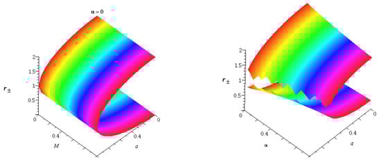
Figure 1.
The figure implies the variation in with a and for the Kerr black hole and the Kerr–MOG black hole. (Left figure) for Kerr black hole. (Right figure) for Kerr–MOG black hole. The presence of the MOG parameter deformed the shape of the horizon radii.
It should be noted that when , one obtains the horizon radii of the Kerr black hole. The black hole solution exists when . When , one obtains the extremal black hole. When , one obtains the naked singularity case.
For the sake of convenience and to show the variation with deformation parameter we can define the spin parameter for the MOG black hole as
The new spin parameter varies with the MOG parameter that can be seen in Figure 2. From the plot, we can infer that there is a restriction on the spin parameter in MOG as
Note that the MOG parameter or deformation parameter () is always positive definite. If we invert the above inequality, we obtain the restriction on .
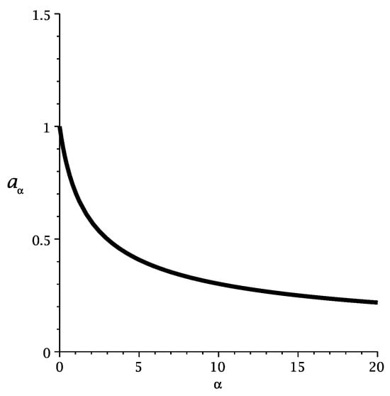
Figure 2.
The figure indicates the variation of spin parameter with , where . This means that the value of the spin parameter decreases when the MOG parameter increases. The maximum value of the MOG parameter is unity. Its value gradually decreases when increases.
For a Kerr black hole, when , there exists a black hole solution. While , it is said to be a naked singularity and when it is said to be an extremal black hole solution. For a Kerr–MOG black hole, these limits can be reduced in the following way. For example, if we take , then these limits are defined as which is the extremal limit, is the naked singularity situation, and is the black hole solution. Similarly, if we take the MOG parameter , then these limits are which is the extremal limit, is the naked singularity situation, and is the black hole solution.
In the below (Table 1), one can find the tabulated values of the spin parameter for various values of the MOG parameter:

Table 1.
Tabulated form of spin limit for non-extremal Kerr-MOG back hole, Extremal Kerr-MOG black hle and Kerr-MOG superspinar.
The outer and inner ergosphere is situated at
and they should satisfy the following inequality .
The structure of the outer and inner ergosphere can be seen visually in Figure 3.
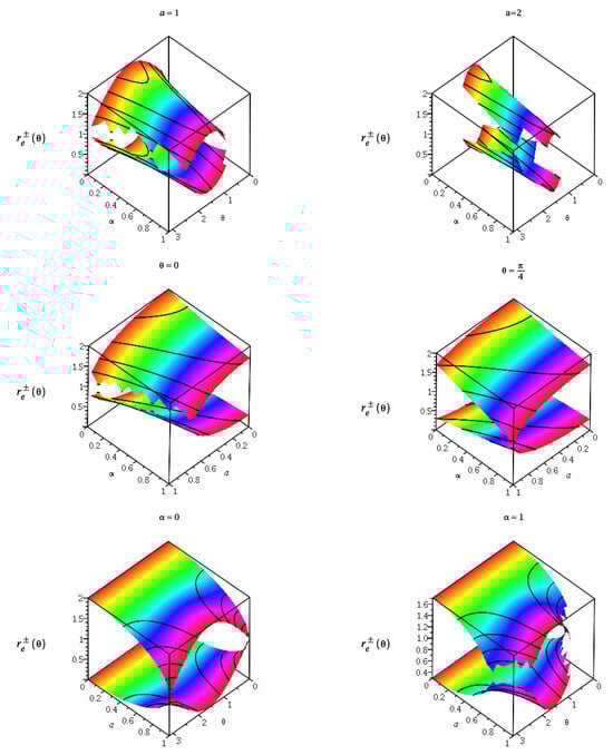
Figure 3.
The figure indicates the variation in with a and for Kerr black hole and Kerr–MOG black hole. In each plot, the upper half corresponds to and the lower half corresponds to .
In the extremal limit, the outer horizon and inner horizon are coincident at . The outer and inner ergosphere radius reduce to
The structure of the equatorial ergosphere can be seen visually in Figure 4. In the limit ,
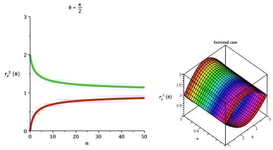
Figure 4.
The figure implies the variation in with for extremal Kerr–MOG black hole in equatorial plane.
This surface is outer to the event horizon or outer horizon and it coincides with the outer horizon at the poles and . The metric components of the above black hole in the Boyer–Lindquist coordinate are
where
and the quantity is defined by
where . Putting these metric components in Equation (15), one obtains the generalized spin precession frequency of a test gyro for the Kerr–MOG black hole
where,
This is the expression of generalized spin frequency which is valid both for outside and inside the ergosphere. Now, we can determine the range of the angular velocity and therefore the four velocity must be time-like, i.e., . The allowed values of at any fixed are where
For the Kerr–MOG black hole, it should be
Now, we calculate the values of when an observer is close to the horizon. At the event horizon, the angular velocity becomes and at the Cauchy horizon the angular velocity becomes . In the equatorial plane
Finally, at the ring singularity and
This means that two angular frequencies coincide at the ring singularity. The variation in the angular frequency () of a stationary gyroscope can be observed from the whale diagram (Figure 5). The significance of the whale diagram is that the whale or a fish can move along the and and it is prominent when the MOG parameter vanishes, i.e., . For details of the whale diagram and escape cones, one can see an interesting work by Tanatorov and Zaslavskii []. We set the value of during the plotting which is valid throughout the work. In Figure 5a–c, we also set the MOG parameter () and will vary the spin parameter value to differentiate three types of compact objects namely non-extremal Kerr, extremal Kerr, and naked singularity. The three pictures are qualitatively different and differentiate between a non-extremal black hole, an extremal black hole, and naked singularity. In Figure 5d–f, we set the value of the MOG parameter as unity. In this case, one can see the variation of angular velocity with the radial coordinate to differentiate three compact objects. Both and are clearly distinct in each case. The distinction is more pronounced in Figure 5a–c and so on for greater values of the MOG parameter.
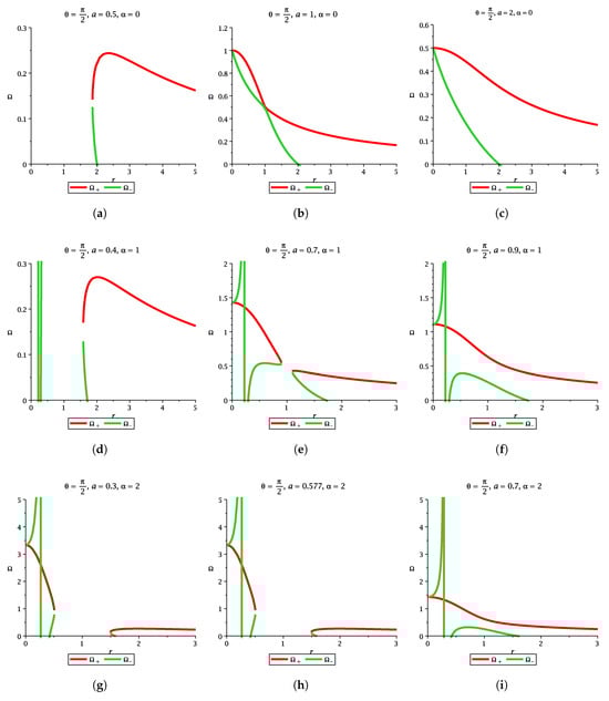
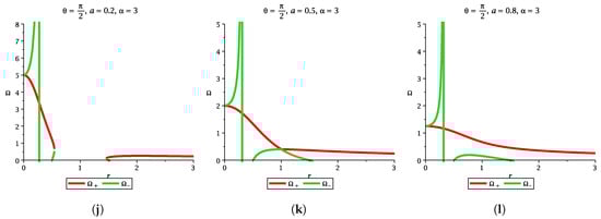
Figure 5.
The figure describes the variation in with r for different values of spin parameter, with the MOG parameter and without the MOG parameter. The gyroscope has angular frequency and varies within the range . Each set of a row depicts the variation in vs r for a non-extremal black hole, an extremal black hole, and naked singularity. There is a qualitative difference between these plots, i.e., when we have taken into account the MOG parameter and without MOG parameter.
The angular frequency has two values, i.e., in the outer horizon it is and in the inner horizon it is . Now, we analyze the behavior of the gyro inside the ergosphere of a black hole and to do this job we should first compute the magnitude of the precession frequency for various values of .
For this purpose, we introduce the parameter to scan the entire range of as
where and . It is evident that the limiting value of gives the range of from to . Using Equation (55), one obtains the generalized spin precession frequency in a compact form
where
The implication of this equation is that one could study the behaviour of generalized spin frequency with spin parameter a, , , r, and MOG parameter. It should be noted that the frequency vector diverges at , , and . This means that the generalized spin precession frequency becomes arbitrarily large at these values. Using this frequency, one should differentiate between the black hole and naked singularity in a strong gravitational field.
Now, consider an observer moving with a four velocity u in a stationary and axisymmetric spacetime. If the angular momentum is zero for a particular situation which is defined by
(where is the Lagrangian and is angular momentum) such an observer is called a zero angular momentum observer (ZAMO) which was first observed by Bardeen [,]. Bardeen et al. [] proved that the ZAMO frame is a powerful tool to analyze the physical processes near the astrophysical object. What happens in the case of Newtonian gravity? The angular momentum and angular velocity are satisfied by the relation . This implies that there is no problem when we take into consideration the non-rotating frame, i.e., . The problem should arise when we consider Einstein’s gravity: in this case, the angular momentum satisfies the following relation , where . Here, we would not obtain when . This indicates that there must exist two different observers, i.e., one should be a zero angular momentum observer (ZAMO) and the other one should be a zero angular velocity observer (ZAVO). In a ZAMO frame, the value of the angular momentum is while in a ZAVO frame, . The frame-dragging angular velocity of these two frames is . One should define the gravitational potential in the ZAMO frame as , where is a contravariant component of a stationary axisymmetric spacetime metric. This potential is again related to the gravitational acceleration (acceleration due to gravity) as felt by an observer in space . The gravitational accelaration is a kinematic invariant quantity. Using Equation (54), one can easily see that for a particular value of the value of the angular velocity for the Kerr–MOG black hole in the ZAMO frame is
This implies that the ZAMO’s angular velocity is a function of the spin parameter and the charge parameter. In the plane, the ZAMO’s angular velocity should be
The variation of and in the equatorial plane can be seen in Figure 5 and Figure 6, respectively. It must be noted that both these parameters are dependent on the MOG parameter. From Figure 5 and Figure 6, it is observed that the three cases non-extremal, extremal, and naked singularity both in the presence of the MOG parameter and in the absence of the MOG parameter are qualitatively different. This means that three geometries are quite distinguished.
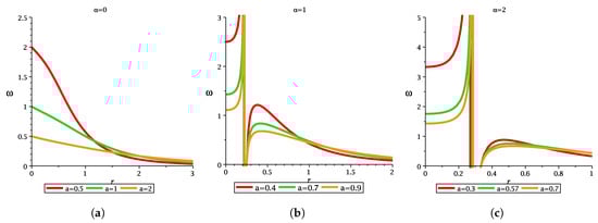
Figure 6.
The figure depicts the variation in with r for different values of the spin parameter in the plane. This frequency is a special class of frequency called ZAMO frequency when . The figure first figure is considered without the MOG parameter () and for various values of the spin parameter to differentiate between a non-extremal black hole, an extremal black hole, and naked singularity. The second and third figure is considered with the MOG parameter and . In the first figure, the ZAMO frequency decreases for each spin value , , and increasing the value of r. In the second figure, the ZAMO frequency first increases then at a certain point it diverges, then it further increases to a certain peak, then decreases (for each spin value).
In this section, we discuss various cases of Generalized Spin Precession Frequency. Also, we see the Generalized Spin Precession Frequency structure for various useful limits. First, we took the limit (i.e., at the ring singularity , ). It should be noted that is not valid at the ring singularity (). Yet, we should investigate its behavior in its vicinity, i.e., in the region , . It must be noted that this region is completely outside the ergoregion since the ergosurface meets the ring singularity. At , the Lense–Thirring precession frequency becomes
and the magnitude of this vector is thus
where
where
and
The valid regime of is
where
where
For a static observer outside the ergosphere, we have to put ; therefore, we obtain from Equation (61)
It must be noted that varies in for at . This indicates that it diverges only at the ring singularity and in cartesian Kerr–Schild coordinates it is described by , while it is finite inside the ring singularity, i.e., [].
2.2. Mathematical Derivation of Generalized Spin Precession Frequency at
In the limit , is given by
where
Using the identity , the above equations reduced to
The magnitude of this vector is calculated to be
From the above equation, one can see that the generalized spin precession frequency is arbitrarily large when . is positive when and negative when and becomes zero when .
For our record, we also compute the generalized spin frequency for various angular limits in the Appendix B, Appendix C, Appendix D.
2.3. Mathematical Derivation of Generalized Spin Precession Frequency at
In the equatorial plane, the generalized spin precession frequency vector is given by
The magnitude of this vector is thus
where
The range of can be determined by using Equation (52). As we said earlier, the outer horizon and the outer ergosurface are located at and , while in the equatorial plane, the ergosphere is located at where and . Therefore, one can obtain the precession frequency at the equatorial ergosurface
where
where
and
where
In the extremal limit , the precession frequency becomes
The value of lies in the range . This indicates that if the central object’s mass or angular momentum increases, then the value of both at the ergosurface and in the plane decreases. This may be written in terms of the MOG parameter as
when the MOG parameter reduces to zero, one obtains the result of the extremal Kerr black hole as . It should be noted that the precession frequency at the outer horizon of the extremal Kerr–MOG black hole is computed to be
In terms of the MOG parameter, the above expression can be written as
When , the precession frequency reduces to an extremal black hole, .
2.4. Generalized Spin Precession Frequency in the Schwarzschild–MOG Spacetime
In the limit , the Kerr–MOG black hole reduces to Schwarzschild–MOG (SMOG) spacetime. In this case, the Generalized Spin Precession Frequency becomes
where might have any value so that u should be timelike.
It must be noted that SMOG spacetime is a spherically symmetric solution of the Einstein equation. It denotes a black hole of mass . In the equatorial plane, becomes
This implies that when a gyroscope is moving in the equatorial plane of the Reissner–Nordström spacetime (static spacetime), it becomes precession frequency. Now, if the gyro moves along circular orbits, then becomes Keplerian frequency, i.e.,
This equation indicates the precession frequency in the Copernican frame which is derived with respect to the proper time . The proper time is computed in the Copernican frame and is related to the coordinate frame t via the relation
Thus, one obtains the precession frequency in the coordinate basis as,
Thus, one can compute the geodetic precession frequency which is the difference between and , and one obtains
This is called the geodetic precession of a test gyroscope around a non-rotating spherical object of mass . In the limit when , one obtains the geodetic precession of the Schwarzschild black hole []. One can see the geodetic precession of a non-rotating spherical object from Figure 7 for different values of the MOG parameter.
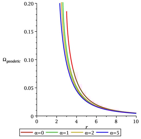
Figure 7.
The figure describes the variation in geodetic precession with r for different values of spin parameter in the plane.
3. Computation of Fundamental Frequencies to Differentiate the Non-Extremal Kerr–MOG, Extremal Kerr–MOG, and Kerr–MOG Superspinar
To distinguish these three geometries of any compact object, it is also essential to study three fundamental frequencies of the accretion disk. This can be possible only by studying the geodesic motion of test particles around the compact objects. To study the physics of the accretion disk, one should compute the said compact object’s stable circular orbit. The prime stable orbit is the innermost stable circular orbit (ISCO) or the last stable circular orbit (LSCO). This ISCO can help us to distinguish these three geometries. In Kerr geometry, the ISCO radii depends on the spin parameter (a) while in Kerr–MOG geometry, it depends on both the spin parameter () and the MOG parameter (). We previously noticed that in Kerr–MOG geometry, the spin parameter decreases as MOG value increases (See Figure 2).
Three fundamental frequencies which are very important for accretion disk physics of the Kerr–MOG black hole, namely the Keplerian frequency (), the radial epicyclic frequency (), and the vertical epicyclic frequency (). This can easily be derived using Formulas (A3), (A5) and (A7) given in Appendix A (See also []) (note that in Ref. [] the term is missing; here, we included it in each frequency formula)
It is important to note the upper sign for the corotating (direct) orbit and the lower sign for the counter-rotating (retrograde) orbit. When the MOG value vanishes, one obtains the epicyclic frequencies of a Kerr black hole.
The variation in these frequencies for three compact objects, namely non-extremal black hole, extremal black hole, and naked singularity, can be seen from the following diagram (Figure 8, Figure 9 and Figure 10). From the first figure, when it means that for the Kerr black hole, it is observed that the Keplerian frequency decreases on increasing the radial value, starting from a maximum value for a non-extremal black hole (). As the spin value increases, the value of the Keplerian frequency decreases. In the second figure, where the MOG parameter is present the picture is quite different from the former. Here the Keplerian frequency has gone through a peak for different spin values.
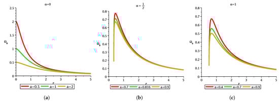
Figure 8.
The figure depicts the variation in with r for different MOG parameter and spin parameter. Each figure demonstrates the difference between non-extremal black hole, extremal black hole, and naked singularity. Without MOG there is no peak while with MOG there exists a peak value in Keplerian frequency.
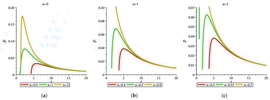
Figure 9.
The figure depicts the variation in with r for different MOG parameter and spin parameter. Each figure shows the difference between three compact objects namely, non-extremal black hole, extremal black hole, and naked singularity.
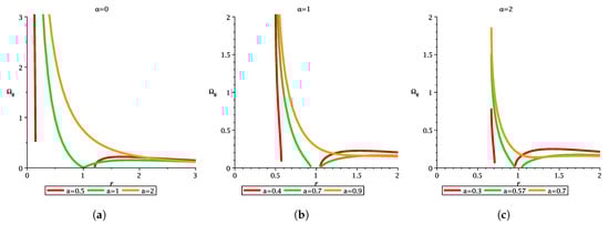
Figure 10.
The figure depicts the variation in with r for different MOG parameter and spin parameter. Each figure characterizes the difference between non-extremal black hole, extremal black hole, and naked singularity.
The other two important frequencies, namely the periastron precession frequency () and nodal precession frequency (), can be defined as
All the above frequencies that we have defined are related to the precession of the orbit and orbital plane. Periastron frequency occurs due to the precession of the orbit while nodal precession frequency occurs due to the precession of the orbital plane. Sometimes, the nodal precession frequency is called the orbital planer precession frequency or the Lense–Thirring precession frequency []. The radial variation of these two frequencies can be observed in Figure 11 and Figure 12.
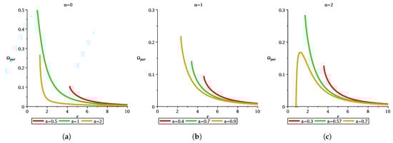
Figure 11.
The figure depicts the variation in with r for different MOG parameter and spin parameter. Each figure shows the difference between non-extremal black hole, extremal black hole, and naked singularity.
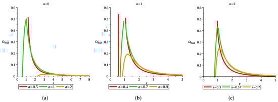
Figure 12.
The figure depicts the variation in with r for different MOG parameter and spin parameter. Each figure classifies the difference between non-extremal black hole, extremal black hole, and naked singularity.
The fact that and determined the stability of circular orbits. From the first condition, one can compute radii of ISCO. It is well known that ISCO of the Kerr black hole is located at []
where
Here, the upper sign indicates direct orbit and the lower sign indicates retrograde orbit. For the extremal Kerr black hole, the ISCO is situated at for direct orbit, while for retrograde orbit []. The non-negativeness of implies that the geodesic motion is stable under small oscillations in the vertical direction. In the Kerr–MOG black hole, the ISCO radii can be calculated via the equation :
To determine the exact ISCO radii of the Kerr–MOG black hole is not a trivial task like the Kerr black hole. So we cannot determine for this black hole. But we expect the condition is satisfied for the Kerr–MOG black hole and while this condition for naked singularity is like the Kerr black hole []. This is one of the main differences between a black hole and naked singularity. But it can be easily checked for without the MOG parameter.
In spherically symmetric spacetime where the value of the spin parameter , it means that , which implies that the Lense–Thirring precession is absent while in axisymmetric spacetime . It would vanish for a particular value of , i.e.,
which implies that
When the MOG parameter vanishes, it reduces to
We can differentiate three compact objects via a ratio of two epicyclic frequencies (plot for direct orbit only) which is defined as follows
The variation in these ratios may be seen from the following diagram (Figure 13, Figure 14 and Figure 15).
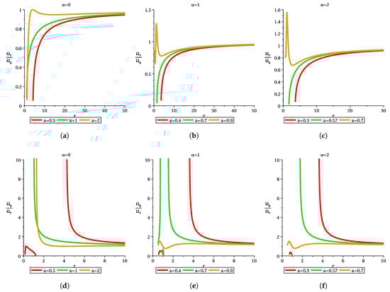
Figure 13.
The figure depicts the variation in and with r for different MOG parameter and spin parameter. Each figure depicts the difference between non-extremal black hole, extremal black hole, and naked singularity.
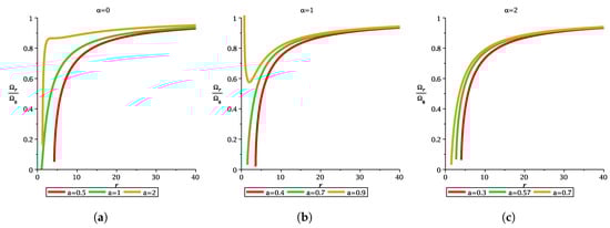
Figure 14.
The figure depicts the variation in with r for different MOG parameter and spin parameter. Each figure depicts the difference between non-extremal black hole, extremal black hole, and naked singularity.
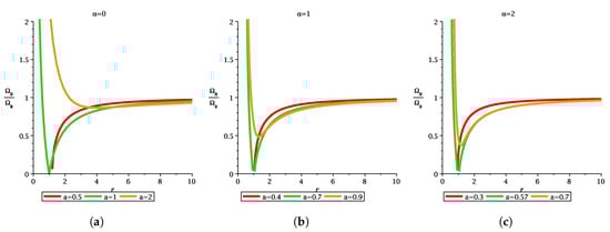
Figure 15.
The figure depicts the variation in with r for different MOG parameter and spin parameter. Each figure depicts the difference between non-extremal black hole, extremal black hole, and naked singularity.
4. Discussion
We computed the generalized spin precession frequency associated with a stationary, axisymmetric Kerr–MOG black hole. Our focus was on calculating the generalized spin precession of a test gyroscope situated within the vicinity of both the black hole and the naked singularity. Through this frequency computation, we were able to differentiate the behaviors of three types of astrophysical compact objects: non-extremal black hole, extremal black hole, and naked singularity or superspinar. We demonstrated a clear visual distinction among these three compact objects. Additionally, we compared our findings with those of the Kerr black hole. Various characteristics of MOG were examined through the analysis of spin precession in relation to the radial profile graph. Each spin precession frequency diagram revealed distinct features of the three compact objects across different spin limits.
One of the most significant outcomes of our research was the identification of the MOG parameter’s influence, which altered the geometric configuration of critical parameters such as the event horizon (), Cauchy horizon (), outer ergosphere (), inner ergosphere (), and the generalized spin precession frequency () when compared to a scenario with a zero MOG parameter. We also explored the generalized spin precession frequency across various angular limits: , , , , and . Furthermore, we investigated the generalized spin frequency for a ring singularity.
In conclusion, we examined the properties of the accretion disks associated with non-extremal Kerr–MOG black hole, extremal Kerr–MOG blackhle, and Kerr–MOG superspinar by calculating three fundamental epicyclic frequencies: the Keplerian frequency, radial epicyclic frequency, and vertical epicyclic frequency. We also analyzed the periastron frequency and nodal frequency. By utilizing these epicyclic frequency properties, we were able to differentiate among the three compact objects. The distinct geometries of these objects were clearly observable from the various frequency diagrams. Additionally, we computed the relevant ratios: , and . Using these features, we differentiated these three compact objects.
The investigation of the stability characteristics of naked singularity within the framework of MOG presents a compelling avenue for research. A recent study, as detailed in reference [], focused on the stability of a superspinar in the context of Kerr geometry. The authors successfully solved the Teukolsky equations and found that the superspinar exhibits stability against linear perturbations specifically for the modes.
In conclusion, to evaluate the effects of strong gravity in MOG and to differentiate among three types of compact objects, namely non-extremal black hole, extremal black hole, and naked singularity or superspinar, we calculated various critical parameters, including , , , , , , , , and . The distinctive features of these parameters enable differentiation between non-extremal black hole, extremal black hole, and superspinar.
Funding
This research received no external funding.
Data Availability Statement
No datasets were generated in this work.
Conflicts of Interest
The authors declare no conflicts of interest.
Appendix A. Epicyclic Frequencies in a General Axisymmetric and Stationary Spacetime
We consider a general stationary and axisymmetric spacetime as
where . For this spacetime, the proper angular momentum () of a test particle can be defined as
where is the orbital frequency of a test particle. Now, can be defined as
The upper sign is for corotating orbit and the lower sign is for counterrotating orbit. The general expressions for computing the radial () and vertical () epicyclic frequencies are [,]
where
and
where
and Z can be defined as
Appendix B. Mathematical Derivation of Generalized Spin Precession Frequency at
In the limit , is computed as
The magnitude of this vector turns out to be
where
Appendix C. Mathematical Derivation of Generalized Spin Precession Frequency at
In the limit , is derived as
The magnitude of this vector is
where
Appendix D. Mathematical Derivation of Generalized Spin Precession Frequency at
In this limit , is computed to be
The magnitude of this vector is given by
where
References
- de Sitter, W. On the bearing of the Principle of Relativity on Gravitational Astronomy. Mon. Not. Roy. Astron. Soc. 1916, 77, 155. [Google Scholar] [CrossRef]
- Lense, J.; Thirring, H. On the effect of rotating distant masses in Einstein’s theory of gravitation. Physikalische Zeitschrift 1918, 19, 156–163. [Google Scholar]
- Schiff, L.I. Possible New Experimental Test of General Relativity Theory. Phys. Rev. Lett. 1960, 4, 215. [Google Scholar] [CrossRef]
- Everitt, C.W.F.; DeBra, D.B.; Parkinson, B.W.; Turneaure, J.P.; Conklin, J.W.; Heifetz, M.I.; Keiser, G.M.; Silbergleit, A.S.; Holmes, T.; Kolodziejczak, J.; et al. Gravity probe B: Final results of a space experiment to test general relativity. Phys. Rev. Lett. 2011, 106, 221101. [Google Scholar] [CrossRef] [PubMed]
- The Rossi X-ray Timing Explorer Mission (1995–2012). Available online: https://heasarc.gsfc.nasa.gov/docs/xte (accessed on 24 December 2024).
- Kannan, R.; Saha, P. Frame dragging and the kinematics of galactic-center stars. Astrophys. J. 2009, 690, 1553. [Google Scholar] [CrossRef]
- de Felice, F.; Tommaset, S.U. Schwarzschild spacetime: Measurements in orbiting space-stations. Class. Quant. Grav. 1993, 10, 353. [Google Scholar] [CrossRef]
- Ciufolini, I.; Wheeler, J.A. Gravitation and Inertia; Princeton University Press: Princeton, NJ, USA, 1995. [Google Scholar]
- Will, C.M. Theory and Experiment in Gravitational Physics, 2nd ed.; Cambridge University Press: Cambridge, UK, 1993. [Google Scholar]
- Ciufolini, I. Dragging of inertial frames. Nature 2007, 449, 41. [Google Scholar] [CrossRef] [PubMed]
- Iorio, L. An Assessment of the Systematic Uncertainty in Present and Future Tests of the Lense–Thirring Effect with Satellite Laser Ranging. Space Sci. Rev. 2009, 148, 363–381. [Google Scholar] [CrossRef]
- Hartle, J.B. Gravity: An Introduction to Einstein’s General Relativity; Pearson: London, UK, 2009. [Google Scholar]
- Chakraborty, C.; Majumdar, P. Strong gravity Lense–Thirring precession in Kerr and Kerr–Taub–NUT spacetimes. Class. Quantum Grav. 2014, 31, 075006. [Google Scholar] [CrossRef]
- Chakraborty, C.; Pradhan, P. Lense–Thirring precession in Plebański-Demiański Spacetimes. Eur. Phys. J. C 2013, 73, 2536. [Google Scholar] [CrossRef]
- Chakraborty, C.; Pradhan, P. Behavior of a test gyroscope moving towards a rotating traversable wormhole. J. Cosmol. Astropart. Phys. JCAP 2017, 003, 035. [Google Scholar] [CrossRef]
- Chakraborty, C.; Modak, K.P.; Bandyopadhyay, D. Dragging of inertial frames inside the rotating neutron stars. Astrophys. J. 2014, 790, 2. [Google Scholar] [CrossRef]
- Morsink, S.M.; Stella, L. Relativistic precession around rotating neutron stars: Effects due to frame-dragging and stellar oblateness. Astrophys. J. 1999, 513, 827. [Google Scholar] [CrossRef]
- Pfister, H. On the history of the so-called Lense–Thirring effect. Gen. Rel. Grav. 2007, 39, 1735–1748. [Google Scholar] [CrossRef]
- Bini, D.; Geralico, A.; Jantzen, R.T. Gyroscope precession along bound equatorial plane orbits around a Kerr black hole. Phys. Rev. D 2016, 94, 064066. [Google Scholar] [CrossRef]
- Chakraborty, C.; Ganguly, O.; Majumdar, P. Inertial Frame Dragging in an Acoustic Analogue Spacetime. Ann. Phys. 2017, 530, 1700231. [Google Scholar] [CrossRef]
- Moffat, J.W. Black Holes in Modified Gravity. Eur. Phys. J. C 2015, 75, 175. [Google Scholar] [CrossRef]
- Moffat, J.W. Modified Gravity Black Holes and their Observable Shadows. Eur. Phys. J. C 2015, 75, 130. [Google Scholar] [CrossRef]
- Mureika, J.R.; Moffat, J.W.; Faizal, M. Black Hole Thermodynamics in Modified Gravity. Phys. Lett. B 2016, 757, 528. [Google Scholar] [CrossRef]
- Wondrak, M.F.; Nicolinia, P.; Moffat, J.W. Superradiance in Modified Gravity (MOG). J. Cosmol. Astropart. Phys. JCAP 2018, 2018, 21. [Google Scholar] [CrossRef]
- Moffat, J.W.; Toth, V.T. The bending of light and lensing in modified gravity. Mon. Not. R. Astron. Soc. MNRAS 2009, 397, 1885. [Google Scholar] [CrossRef]
- Manfredi, L.; Mureika, J.; Moffat, J. Quasinormal modes of modified gravity (MOG) black holes. Phys. Lett. B 2018, 779, 492. [Google Scholar] [CrossRef]
- Moffat, J.W. Scalar-Tensor-Vector Gravity Theory. J. Cosmol. Astropart. Phys. JCAP 2006, 0603, 004. [Google Scholar] [CrossRef]
- Pradhan, P. Area (or Entropy) Products in Modified Gravity and Kerr–MOG/CFT Correspondence. Euro. Phys. J. Plus 2018, 133, 187. [Google Scholar] [CrossRef]
- Wei, S.W.; Liu, Y.X. Merger estimates for rotating Kerr black holes in modified gravity. Phys. Rev. D 2018, 98, 024042. [Google Scholar] [CrossRef]
- Sheoren, P.; Aguilar, A.H.; Nucamendi, U. Mass and spin of a Kerr black hole in modified gravity and a test of the Kerr black hole hypothesis. Phys. Rev. D 2018, 97, 124049. [Google Scholar] [CrossRef]
- Pradhan, P. Study of energy extraction and epicyclic frequencies in Kerr–MOG (Modified Gravity) black hole. Eur. Phys. J. C 2019, 79, 401. [Google Scholar] [CrossRef]
- Nozari, K.; Saghafi, S.; Mohammadpour, A. Higher-Dimensional MOG dark compact object: Shadow behavior in the light of EHT observations. arXiv 2024, arXiv:2407.06393. [Google Scholar] [CrossRef]
- Chakraborty, C.; Kocherlakota, P.; Patil, M.; Bhattacharyya, S.; Joshi, P.S.; Królak, A. Distinguishing Kerr naked singularities and black holes using the spin precession of a test gyro in strong gravitational fields. Phys. Rev. 2017, 95, 084024. [Google Scholar] [CrossRef]
- Chakraborty, C.; Kocherlakota, P.; Joshi, P.S. Spin precession in a black hole and naked singularity spacetime. Phys. Rev. D 2017, 95, 044006. [Google Scholar] [CrossRef]
- Pugliese, D.; Quevedo, H.; Ruffini, R. Equatorial circular orbits of neutral test particles in the Kerr–Newman spacetime. Phys. Rev. D 2013, 88, 024042. [Google Scholar] [CrossRef]
- de Felice, F. Classical instability of a naked singularity. Nature 1978, 273, 8. [Google Scholar] [CrossRef]
- Calvini, M.; de Felice, F.; Nobili, L. Are Naked Singularities Really Visible? Lett. Nuovo Cimento 1978, 23, 15. [Google Scholar] [CrossRef]
- Zhang, H. Naked Singularity, firewall, and Hawking radiation. Sci. Rep. 2017, 7, 4000. [Google Scholar] [CrossRef] [PubMed]
- Pugliese, D.; Quevedo, H. Disclosing connections between black holes and naked singularities: Horizon remnants, Killing throats and bottlenecks. Eur. Phys. J. C 2019, 79, 209. [Google Scholar] [CrossRef]
- Pugliese, D.; Quevedo, H. Kerr metric bundles. Killing horizons confinement, light-surfaces, and horizons replicas. arXiv 2020, arXiv:2005.04130. [Google Scholar]
- Pradhan, P. Distinguishing signature of Kerr–MOG black hole and superspinar via Lense–Thirring precession. Euro. Phys. J. C 2024, 84, 841. [Google Scholar] [CrossRef]
- Pradhan, P.; Moffat, J. Zero Mass Limit of Kerr–MOG Black Hole Equals Wormhole. arXiv 2024, arXiv:2412.08844. [Google Scholar]
- Maselli, A.; Pani, P.; Cotesta, R.; Gualtieri, L.; Ferrari, V.; Stella, L. Geodesic models of quasi-periodic-oscillations as probes of quadratic gravity. Astrophys. J. 2017, 1, 843. [Google Scholar] [CrossRef]
- Stella, L.; Vietri, M.; Morsink, S. Correlations in the QPOs frequencies of low mass x-ray binaries and the relativistic precession model. Astrophys. J. 1999, L63–L66, 524. [Google Scholar]
- Török, G.; Stuchlik, Z. Radial and vertical epicyclic frequencies of Keplerian motion in the field of Kerr naked singularities. Astron. Astrophys. 2005, 437, 775. [Google Scholar] [CrossRef]
- Straumann, N. General Relativity with Applications to Astrophysics; Springer: Berlin/Heidelberg, Germany, 2009. [Google Scholar]
- Jantzen, R.T.; Carini, P.; Bini, D. The Many Faces of Gravitoelectromagnetism. Annals Phys. 1992, 215, 1. [Google Scholar] [CrossRef]
- Chatterjee, D.; Chakraborty, C.; Bandyopadhyay, D. Gravitomagnetic effect in magnetized neutron stars. J. Cosmol. Astropart. Phys. JCAP 2017, 01, 062. [Google Scholar] [CrossRef][Green Version]
- Tanatarov, I.V.; Zaslavskii, O.B. Collisional super-Penrose Process and Wald inequalities. Gen. Relat. Gravit. 2017, 49, 119. [Google Scholar] [CrossRef][Green Version]
- Bardeen, J.M. A Variational Principle for Rotating Stars in General Relativity. Astrophys. J. 1970, 162, 71. [Google Scholar] [CrossRef]
- Misner, C.W.; Thorne, K.S.; Wheeler, J.A. Gravitation; W. H. Freeman & Company: New York City, NY, USA, 1973. [Google Scholar]
- Bardeen, J.M.; Press, W.H.; Teukolsky, S.A. Rotating Black Holes: Locally Non-rotating Frames, Energy Extraction, and Scalar Synchrotron Radiation. Astrophys. J. 1972, 178, 347. [Google Scholar] [CrossRef]
- Sakina, K.; Chiba, J. Parallel transport of a vector along a circular orbit in Schwarzschild space-time. Phys. Rev. D 1979, 19, 2280. [Google Scholar] [CrossRef]
- Nakao, K.-I.; Joshi, P.S.; Guo, J.-Q.; Kocherlakota, P.; Tagoshi, H.; Harada, T.; Patil, M.; Królak, A. On the stability of a superspinar. Phys. Lett. B. 2018, 780, 410. [Google Scholar] [CrossRef]
- Doneva, D.D.; Yazadjiev, S.S.; Stergioulas, N.; Kokkotas, K.D.; Athanasiadis, T.M. Orbital and epicyclic frequencies around rapidly rotating compact stars in scalar-tensor theories of gravity. Phys. Rev. 2014, 90, 044004. [Google Scholar] [CrossRef]
Disclaimer/Publisher’s Note: The statements, opinions and data contained in all publications are solely those of the individual author(s) and contributor(s) and not of MDPI and/or the editor(s). MDPI and/or the editor(s) disclaim responsibility for any injury to people or property resulting from any ideas, methods, instructions or products referred to in the content. |
© 2024 by the author. Licensee MDPI, Basel, Switzerland. This article is an open access article distributed under the terms and conditions of the Creative Commons Attribution (CC BY) license (https://creativecommons.org/licenses/by/4.0/).