Accelerated Reliability Growth Test for Magnetic Resonance Imaging System Using Time-of-Flight Three-Dimensional Pulse Sequence


Abstract
:1. Introduction
2. Related work
2.1. Magnetic Resonance Imaging (MRI) System Brief Overview
2.2. Types of Reliability Test
2.2.1. Reliability Growth Test
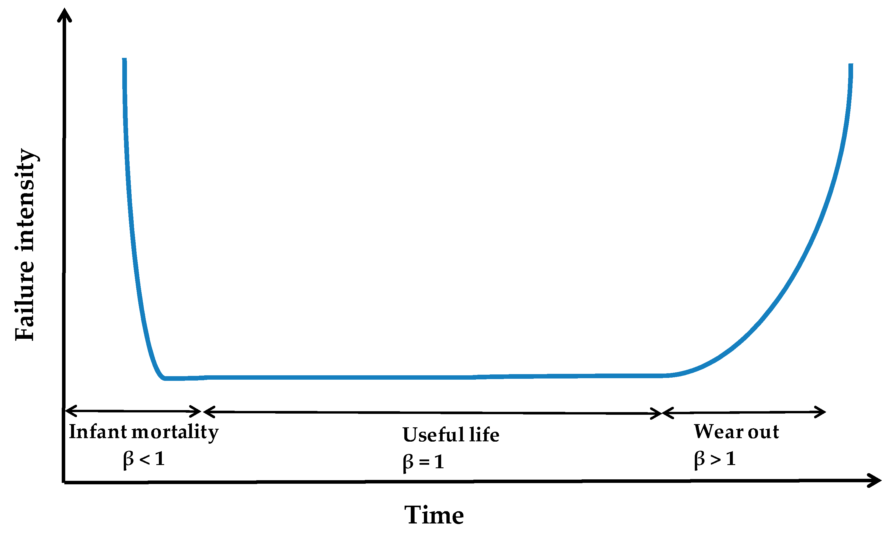
2.2.2. Reliability Growth Test Using Crow AMSAA Model
- λ = Failure intensity
- α = Scale parameter
- β = Shape parameter
- N = Total number of failures
- t = Test time
- Ts = Total test time
- Ti = Time at ith failure occurring
2.2.3. Reliability Demonstration Test
2.2.4. Accelerated Life Test
- AF1 = Acceleration factor due to stress parameter 1
- AF2 = Acceleration factor due to stress parameter 2
- AFn = Acceleration factor due to stress parameter n
- AF = Total acceleration factor
- L = Product life
- s = Sample size
- T = Test time
3. Proposed MRI System Accelerated Reliability Growth Test
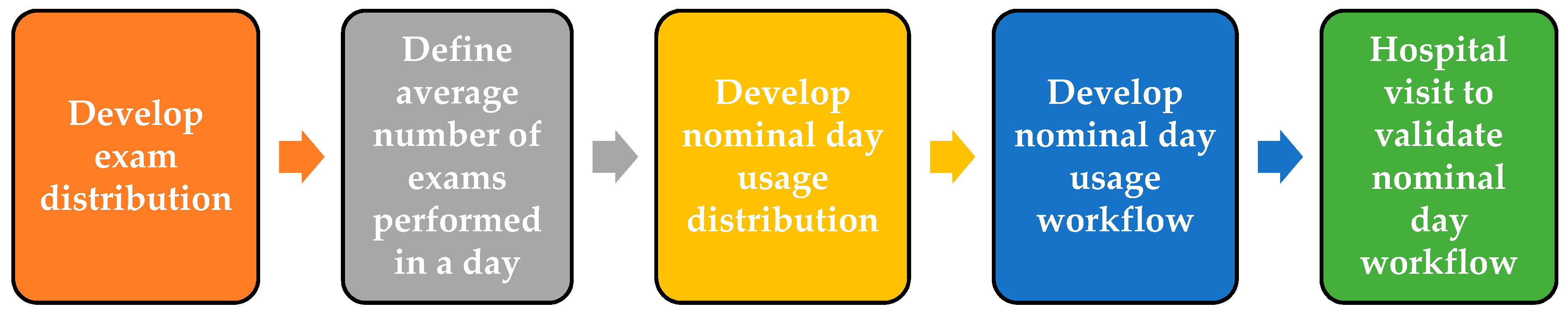
3.1. Development of Nominal Day Usage Scenario for a MRI System
- Hospital 1: 50,867 exams on 8 MRI systems in a year
- Hospital 2: 53,099 exams on 8 MRI systems in a year
- NHS, England (Multiple Hospitals): 1,980,000 exams on 304 systems [26]
3.1.1. MRI Exam Distribution
3.1.2. Average Number of MRI Exams in a Day
- Number of exams per day per system in Hospital 1 =
- Number of exams per day per system in Hospital 2 =
- Number of exams per day per system as per NHS data =
- Average number of exams per day =
3.1.3. Nominal Day Usage Distribution
3.1.4. Nominal Day Usage Workflow
3.1.5. Hospital Visit to Validate the Workflow
3.2. MRI System Reliability Growth Test and Current Challenges
- L = MRI system life in years
- W = Number of weeks per year for MRI system usage
- D = Number of nominal days per week MRI System usage
- n = Number of exams performed in a nominal day
- m = Number of pulse sequence in each exam
- i = ith exam performed in a nominal day
- j = jth pulse sequence
- PSij = jth pulse sequence of ith exam
- Tij = Time taken by jth pulse sequence in ith exam
- TD = Time to complete all exams in a nominal day
- T = Time (in days) to complete the reliability growth test
- H = Number of test hours in a day
- L = 10 years
- W = 50 weeks/year
- D = 6 days/week
- n = 21
- H = 24 h
3.3. MRI System Stress Parameters and Life-Time Stress Analysis
3.3.1. Identifying Stress Parameters
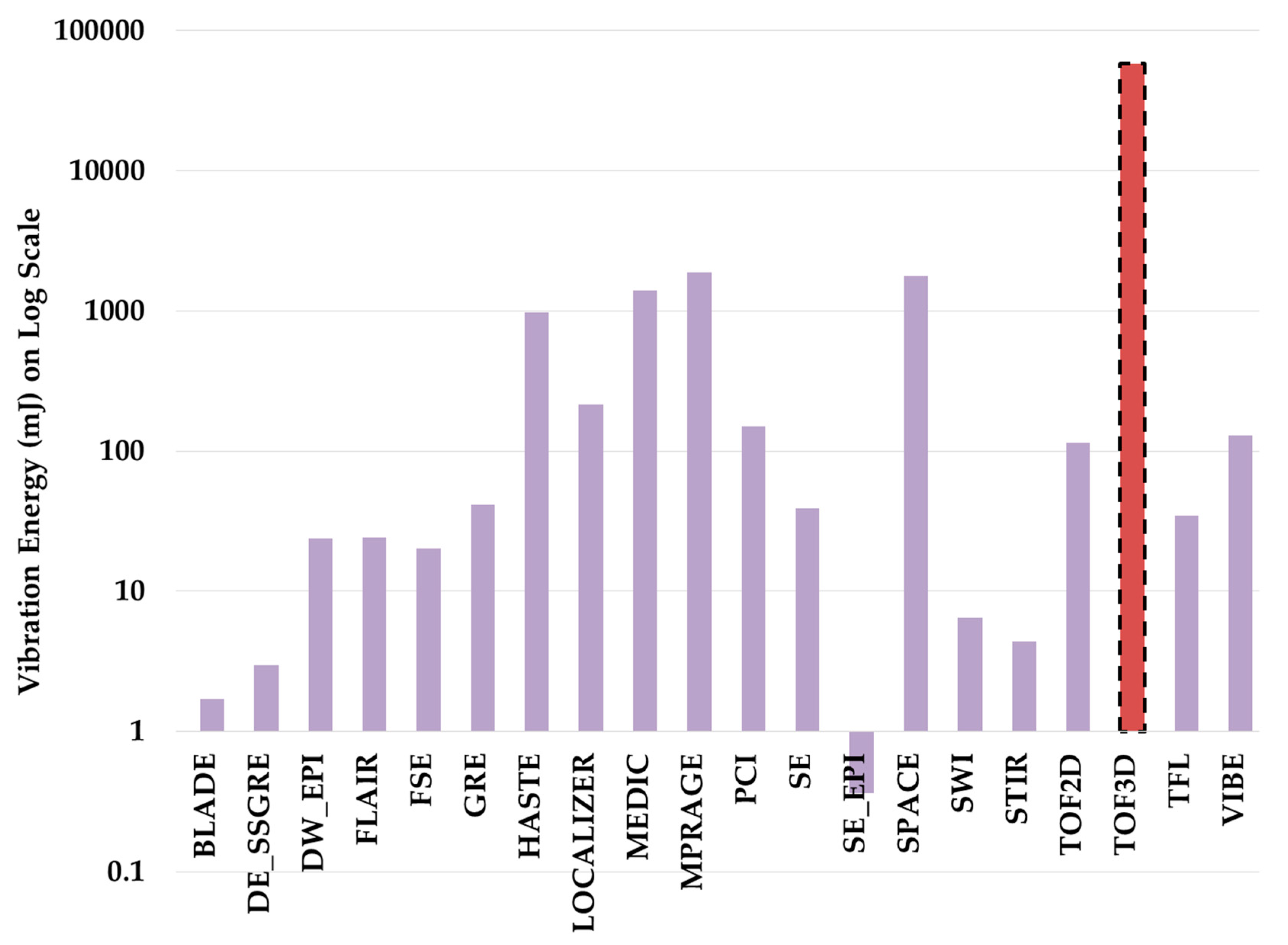
3.3.2. Establishing Relation Between Pulse Sequences and Vibration Energy
3.3.3. Life-Time Analysis using Vibration Energy
- VEij = Vibration energy exerted on gradient coil during jth pulse sequence in ith exam
- VED = Total vibration energy exerted on gradient coil in a nominal day
- VET = Total vibration energy exerted on gradient coil in entire life
3.4. MRI System Accelerated Reliability Growth Test
3.4.1. Developing Test Cycle to Accelerate the Reliability Test
3.4.2. Calculating Acceleration Factor and Test Duration
- VEc = Total vibration energy in a test cycle
- VED = Total vibration energy exerted on gradient coil in a nominal day
- p = Inverse square law coefficient for vibration
- Tc = Time to complete one test cycle
- H = Number of test hours in a day
- T = Time (in days) to complete the reliability growth test
- AFV = Acceleration factor due to vibration energy
- AFT = Acceleration factor due to time
- AF = Total acceleration factor
- s = Sample size (Number of test sample)
- L = MRI system life in years
- W = Number of weeks per year for MRI system usage
- D = Number of nominal days per week MRI System usage
- n = Number of exams performed in a nominal day
- m = Number of pulse sequence in each exam
- i = ith exam performed in a nominal day
- j = jth pulse sequence
- PSij = jth pulse sequence of ith exam
- VEij = Vibration energy exerted on gradient coil during jth pulse sequence in ith exam
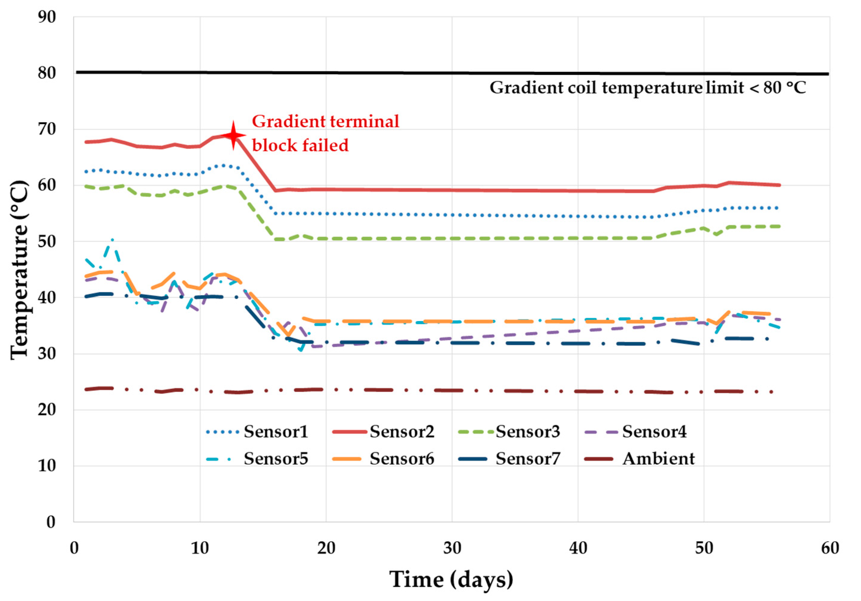
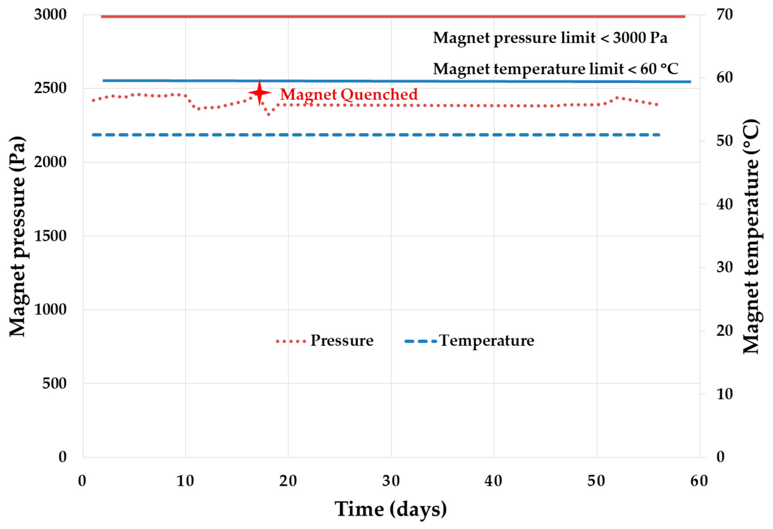
3.4.3. Performing an Accelerated Reliability Growth Test
- Magnet pressure;
- Magnet body temperature;
- Gradient coil temperature;
- Heat exchanger unit coolant temperature;
- RF amplifier coolant temperature;
- Gradient amplifier coolant temperature;
- Gradient coil coolant temperature;
- Several other parameters for software and system.
4. Accelerated Reliability Growth Test Result and Discussion
4.1. Magnet Subsystem Performance
4.2. Gradient Subsystem Performance
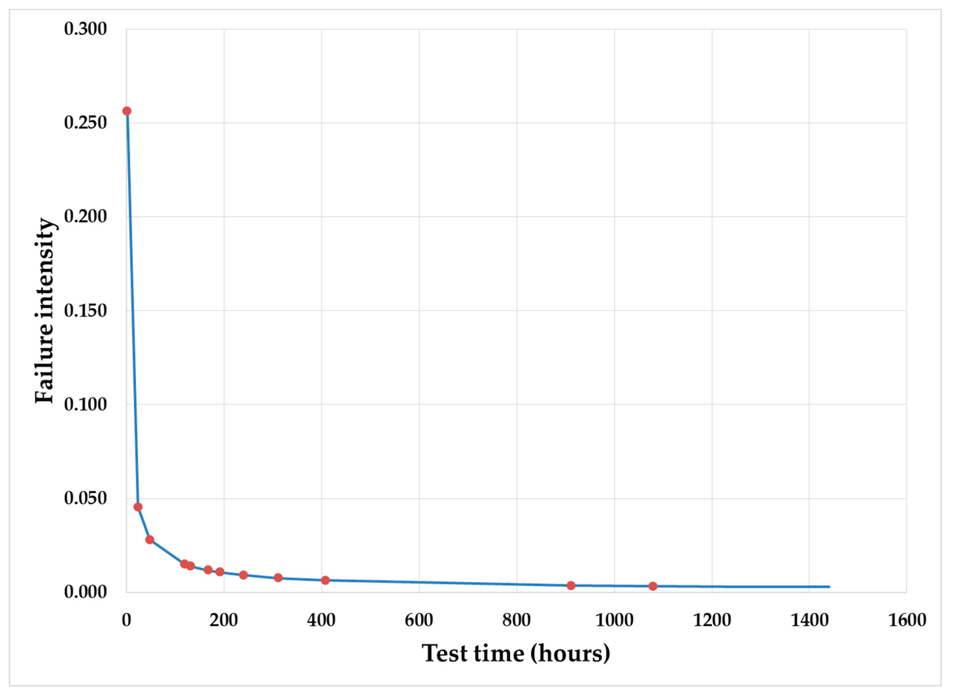
4.3. Crow AMSAA Plot
- N = 12
- Ts = 1440 h
- Ti = 2, 24, ….., 1080 h
5. Conclusions
Author Contributions
Funding
Acknowledgments
Conflicts of Interest
References
- Sinanna, A.; Belorgey, J.; Bredy, P.; Donati, A.; Dubois, O.; Guihard, Q.; Lannou, H.; Lotode, A.; Guiho, P.; Touzery, R.; et al. High reliability and availability of the Iseult/INUMAC MRI magnet facility. IEEE Trans. Appl. Supercond. 2016, 26, 1–5. [Google Scholar] [CrossRef]
- Zhang, J.; Ma, X.; Zhao, Y. Reliability demonstration for long-life products based on hardened testing method and gamma process. IEEE Access. 2017, 5, 19322–19332. [Google Scholar] [CrossRef]
- Sayed, A.; El-Shimy, M.; El-Metwally, M.; Elshahed, M. Reliability, Availability and Maintainability Analysis for Grid-Connected Solar Photovoltaic Systems. Energies 2019, 12, 1213. [Google Scholar] [CrossRef]
- Wang, P.; Coit, D.W. Repairable systems reliability trend tests and evaluation. In Proceedings of the Annual Reliability and Maintainability Symposium, Alexandria, VA, USA, 24 January 2005; pp. 416–421. [Google Scholar]
- Xing, Y.Y.; Wu, X.Y.; Jiang, P.; Liu, Q. Dynamic Bayesian evaluation method for system reliability growth based on in-time correction. IEEE Trans. Reliab. 2010, 59, 309–312. [Google Scholar] [CrossRef]
- Almering, V.; van Genuchten, M.; Cloudt, G.; Sonnemans, P.J. Using software reliability growth models in practice. IEEE softw. 2007, 24, 82–88. [Google Scholar] [CrossRef]
- Duane, J.T. Learning curve approach to reliability monitoring. IEEE Trans. Aerosp. 1964, 2, 563–566. [Google Scholar] [CrossRef]
- Crow, L.H. Reliability Analysis for Complex, Repairable Systems. Army Materiel Systems Analysis Activityaberdeen Proving Ground MD. 1975. Available online: https://pdfs.semanticscholar.org/e176/06aeb2e7c003ad1b7610006bbb27ac622a10.pdf (accessed on 24 October 2019).
- Sun, A.; Kee, E.; Yu, W.; Popova, E.; Grantom, R.; Richards, D. Application of Crow-AMSAA analysis to nuclear power plant equipment performance. In Proceedings of the Nuclear Engineering ICONE-13, Beijing, China, 16 May 2005; pp. 16–20. [Google Scholar]
- Barringer, H.P. Use Crow-AMSAA Reliability Growth Plots to Forecast Future System Failures. Available online: http://citeseerx.ist.psu.edu/viewdoc/summary?doi=10.1.1.544.4293 (access on 24 October 2019).
- Tang, Z.; Zhou, W.; Zhao, J.; Wang, D.; Zhang, L.; Liu, H.; Yang, Y.; Zhou, C. Comparison of the Weibull and the crow-AMSAA model in prediction of early cable joint failures. IEEE Trans. Power Deliv. 2015, 30, 2410–2418. [Google Scholar] [CrossRef]
- Khan, N.; Aslam, M.; Khan, M.; Jun, C.H. A Variable Control Chart under the Truncated Life Test for a Weibull Distribution. Technologies 2018, 6, 55. [Google Scholar] [CrossRef]
- Fertell, R.; Ershad, H. Automatically Monitoring, Controlling, and Reporting Status/Data for Multiple Product Life Test Stands. Inventions 2019, 4, 7. [Google Scholar] [CrossRef]
- Liu, J.; Zhang, M.; Zhao, N.; Chen, A. A reliability assessment method for high speed train electromagnetic relays. Energies 2018, 11, 652. [Google Scholar] [CrossRef]
- Suhir, E. To Burn-In, or Not to Burn-In: That’s the Question. Aerospace 2019, 6, 29. [Google Scholar] [CrossRef]
- Military, Standard. MIL-HDBK-189. Reliability Growth Management. 1981. Available online: http://everyspec.com/MIL-HDBK/MIL-HDBK-0099-0199/MIL-HDBK-189_NOTICE-1_23581/ (access on 24 October 2019).
- Freind, H. Reliability growth test planning. Inst. Environ. Sci. 1995 1995, 41, 104. [Google Scholar]
- Bothwell, R.; Donthamsetty, R.; Kania, Z.; Wesoloski, R. Reliability evaluation: A field experience from Motorola’s cellular base transceiver systems. In Proceedings of the 1996 Annual Reliability and Maintainability Symposium, Las Vegas, NV, USA, 22–25 January 1996; pp. 348–359. [Google Scholar]
- Hall, J.B.; Mosleh, A. An analytical framework for reliability growth of one-shot systems. Reliab. Eng. Syst. Saf. 2008, 93, 1751–1760. [Google Scholar] [CrossRef]
- Yang, Y. Life Cycle Reliability Engineering; Wiley: Hoboken, NJ, USA, 2007. [Google Scholar]
- Meeker, W.Q.; Hahn, G.J.; Doganaksoy, N. Planning life tests for reliability demonstration. Qual. Prog. 2004, 37, 80. [Google Scholar]
- Sun, Q.; Zhang, Z.; Feng, J.; Pan, Z. A zero-failure reliability demonstration approach based on degradation data. In Proceedings of the 2012 International Conference on Quality, Reliability, Risk, Maintenance, and Safety Engineering, Chengdu, China, 15 June 2012; pp. 947–952. [Google Scholar]
- Nelson, W. Accelerated life testing-step-stress models and data analyses. IEEE Trans. Reliab. 1980, 29, 103–108. [Google Scholar] [CrossRef]
- Ecker, M.; Gerschler, J.B.; Vogel, J.; Käbitz, S.; Hust, F.; Dechent, P.; Sauer, D.U. Development of a lifetime prediction model for lithium-ion batteries based on extended accelerated aging test data. J. Power Sources 2012, 215, 248–257. [Google Scholar] [CrossRef]
- Accelerated Testing with the Inverse Power Law, ReliaSoft. Available online: https://www.reliasoft.com/resources/resource-center/accelerated-testing-with-the-inverse-power-law (accessed on 3 December 2017).
- Diagnostic Imaging Dataset, National Health Service, England. Available online: https://www.england.nhs.uk/statistics/statistical-work-areas/diagnostic-imaging-dataset/ (accessed on 20 September 2016).
- What is the Organ Distribution of MRI Studies? Magnetic Resonance. Available online: https://www.magnetic-resonance.org/ch/21-01.html (accessed on 24 September 2016).


| Exam Type | Hospital 1 | Hospital 2 | EMRF [27] | NHS [26] | Normalized Distribution |
|---|---|---|---|---|---|
| Brain | 50 | 43 | 25 | 29 | 32 |
| Head/Neck | 6 | 1 | 6 | 9 | 7 |
| Spine | 15 | 15 | 25 | 36 | 19 |
| Extremities | 7 | 6 | 20 | 11 | |
| MR Angio | 0 | 15 | 9 | 0 | 8 |
| Abdomen | 19 | 10 | 8 | 15 | 14 |
| Other | 4 | 9 | 7 | 11 | 9 |
| Exam Number (#) | Exam Type | Target Diagnosis |
|---|---|---|
| 1 | Brain | Transient ischemic attack |
| 2 | Brain | Demyelinating |
| 3 | Brain | Routine |
| 4 | Brain | Routine with contrast |
| 5 | Brain | Brain tumor |
| 6 | Brain | Transient ischemic attack |
| 7 | Brain | Demyelinating |
| 8 | Brain | Routine |
| 9 | Brain | Routine with contrast |
| 10 | Brain | Brain tumor |
| 11 | Head and neck | Head and neck routing |
| 12 | Spine | Cervical basic |
| 13 | Spine | Thoracic spin basic |
| 14 | Spine | Lumber trauma |
| 15 | Extremities | Knee meniscus |
| 16 | Extremities | Shoulder |
| 17 | Abdomen and liver | General abdomen/pelvis |
| 18 | Abdomen and liver | Liver routine |
| 19 | Abdomen and liver | Liver steatosis/fibrosis |
| 20 | Angiography | Brain angiography |
| 21 | Angiography | Whole body angiography |
| # | Exam Type | Target Diagnosis | Contrast | Coil Type | Description/Scan Protocol |
|---|---|---|---|---|---|
| 1 | Brain | Transient Ischemic | No | Head | Patient go inside scan room |
| 1 | Brain | Transient Ischemic | No | Head | Patient lie down, RF coil setup |
| 1 | Brain | Transient Ischemic | No | Head | Table moved up and slide in |
| 1 | Brain | Transient Ischemic | No | Head | Turn on laser, Patient landmark |
| 1 | Brain | Transient Ischemic | No | Head | Table moved to home position |
| 1 | Brain | Transient Ischemic | No | Head | Localizer |
| 1 | Brain | Transient Ischemic | No | Head | Set the FOV and any parameters |
| 1 | Brain | Transient Ischemic | No | Head | T1 SE TRA |
| 1 | Brain | Transient Ischemic | No | Head | T2 Flair TRA |
| 1 | Brain | Transient Ischemic | No | Head | T2 TSE TRA |
| 1 | Brain | Transient Ischemic | No | Head | DWI |
| 1 | Brain | Transient Ischemic | No | Head | T2* FL2D TRA |
| 1 | Brain | Transient Ischemic | No | Head | Image review and saved to PACS |
| 1 | Brain | Transient Ischemic | No | Head | Table slide out and lowered down |
| 1 | Brain | Transient Ischemic | No | Head | RF coil removed |
| 1 | Brain | Transient Ischemic | No | Head | Patient moved from scan room |
| 1 | Brain | Transient Ischemic | No | Head | Break time |
| 2 | Brain | Demyelinating | No | Head | Patient go inside scan room |
| 2 | Brain | Demyelinating | No | Head | Patient lie down, RF coil setup |
| 2 | Brain | Demyelinating | No | Head | Table moved up and slide in |
| 2 | Brain | Demyelinating | No | Head | Turn on laser, Patient landmark |
| 2 | Brain | Demyelinating | No | Head | Table moved to home position |
| 2 | Brain | Demyelinating | No | Head | Localizer |
| . | . | . | . | . | . |
| . | . | . | . | . | . |
| . | . | . | . | . | . |
| 21 | MR Angio | Whole Body Angio | No | Multiple | FL3D VIBE @ Top |
| 21 | MR Angio | Whole Body Angio | No | Multiple | FL3D COR PRE POST @ Top |
| 21 | MR Angio | Whole Body Angio | No | Multiple | Image review & saved to PACS |
| 21 | MR Angio | Whole Body Angio | No | Multiple | Table slide out & lowered down |
| 21 | MR Angio | Whole Body Angio | No | Multiple | RF coil removed |
| 21 | MR Angio | Whole Body Angio | No | Multiple | Patient moved from scan room |
| # | Exam Type | Target Diagnosis | Pulse Sequence | Pulse Sequence Time (s) | Vibration Energy (Joule) |
|---|---|---|---|---|---|
| 1 | Brain | Transient Ischemic | Localizer | 12.4 | 0.214 |
| 1 | Brain | Transient Ischemic | T1 SE TRA | 76.9 | 0.039 |
| 1 | Brain | Transient Ischemic | T2 Flair TRA | 145.5 | 0.024 |
| 1 | Brain | Transient Ischemic | T2 TSE TRA | 17.5 | 0.02 |
| 1 | Brain | Transient Ischemic | DWI | 161.5 | 0.024 |
| 1 | Brain | Transient Ischemic | T2*_FL2D_TRA | 4.1 | 0.041 |
| 1 | Brain | Transient Ischemic | Break time | 306 | 0 |
| 2 | Brain | Demyelinating | Localizer | 12.4 | 0.214 |
| 2 | Brain | Demyelinating | T1 SE TRA | 76.9 | 0.039 |
| 2 | Brain | Demyelinating | T2 Flair TRA | 145.5 | 0.024 |
| 2 | Brain | Demyelinating | T2 Flair SAG | 145.5 | 0.024 |
| 2 | Brain | Demyelinating | T2 TSE TRA | 17.5 | 0.02 |
| 2 | Brain | Demyelinating | T1 SE TRA | 76.9 | 0.039 |
| 2 | Brain | Demyelinating | Break time | 306 | 0 |
| . | . | . | . | . | . |
| . | . | . | . | . | . |
| 21 | MR Angio | Whole Body Angio | Localizer @ Bottom | 12.4 | 0.214 |
| 21 | MR Angio | Whole Body Angio | Localizer @ Middle | 12.4 | 0.214 |
| 21 | MR Angio | Whole Body Angio | Localizer @ Top | 12.4 | 0.214 |
| 21 | MR Angio | Whole Body Angio | FL3D COR @ Bottom | 4.1 | 0.041 |
| 21 | MR Angio | Whole Body Angio | FL3D COR @ Middle | 4.1 | 0.041 |
| 21 | MR Angio | Whole Body Angio | FL3D COR @ Top | 4.1 | 0.041 |
| 21 | MR Angio | Whole Body Angio | FL3D VIBE @ Bottom | 41.5 | 0.128 |
| 21 | MR Angio | Whole Body Angio | FL3D COR @ Bottom | 4.1 | 0.041 |
| 21 | MR Angio | Whole Body Angio | FL3D VIBE @ Middle | 41.5 | 0.128 |
| 21 | MR Angio | Whole Body Angio | FL3D COR @ Middle | 4.1 | 0.041 |
| 21 | MR Angio | Whole Body Angio | FL3D VIBE @ Top | 41.5 | 0.128 |
| 21 | MR Angio | Whole Body Angio | FL3D COR @ Top | 4.1 | 0.041 |
| 15387 Sec | 193.3 Joule | ||||
| TD | VED |
| Pulse Sequence (PS) | PS Time (s) | Vibration Energy (Joules) | Cumulative Vibration Energy (Joules) |
|---|---|---|---|
| TOF3D | 410 | 58.03 | 58.03 |
| Idle Time | 60 | 0 | 58.03 |
| TOF3D | 410 | 58.03 | 116.059 |
| Idle Time | 60 | 0 | 116.059 |
| TOF3D | 410 | 58.03 | 174.089 |
| Idle Time | 60 | 0 | 174.089 |
| TOF3D | 410 | 58.03 | 232.118 |
| Idle Time | 60 | 0 | 232.118 |
| TOF3D | 410 | 58.03 | 290.148 |
| Idle Time | 60 | 0 | 290.148 |
| TOF3D | 410 | 58.03 | 348.177 |
| Idle Time | 60 | 0 | 348.177 |
| TOF3D | 410 | 58.03 | 406.207 |
| Idle Time | 60 | 0 | 406.207 |
| TOF3D | 410 | 58.03 | 464.236 |
| Idle Time | 60 | 0 | 464.236 |
| TOF3D | 410 | 58.03 | 522.266 |
| Idle Time | 60 | 0 | 522.266 |
| TOF3D | 410 | 58.03 | 580.295 |
| Break | 3600 | 0 | 580.295 |
| 8240 s (Tc) | 580.3 Joules (VEc) |
© 2019 by the authors. Licensee MDPI, Basel, Switzerland. This article is an open access article distributed under the terms and conditions of the Creative Commons Attribution (CC BY) license (http://creativecommons.org/licenses/by/4.0/).
Share and Cite
Anand, P.K.; Shin, D.R.; Saxena, N.; Memon, M.L. Accelerated Reliability Growth Test for Magnetic Resonance Imaging System Using Time-of-Flight Three-Dimensional Pulse Sequence. Diagnostics 2019, 9, 164. https://doi.org/10.3390/diagnostics9040164
Anand PK, Shin DR, Saxena N, Memon ML. Accelerated Reliability Growth Test for Magnetic Resonance Imaging System Using Time-of-Flight Three-Dimensional Pulse Sequence. Diagnostics. 2019; 9(4):164. https://doi.org/10.3390/diagnostics9040164
Chicago/Turabian StyleAnand, Pradeep Kumar, Dong Ryeol Shin, Navrati Saxena, and Mudasar Latif Memon. 2019. "Accelerated Reliability Growth Test for Magnetic Resonance Imaging System Using Time-of-Flight Three-Dimensional Pulse Sequence" Diagnostics 9, no. 4: 164. https://doi.org/10.3390/diagnostics9040164
APA StyleAnand, P. K., Shin, D. R., Saxena, N., & Memon, M. L. (2019). Accelerated Reliability Growth Test for Magnetic Resonance Imaging System Using Time-of-Flight Three-Dimensional Pulse Sequence. Diagnostics, 9(4), 164. https://doi.org/10.3390/diagnostics9040164