
Brain Cancer Prediction Based on Novel Interpretable Ensemble Gene Selection Algorithm and Classifier

 ,
,  ,
,  , ,
, , 
Abstract
:1. Introduction
- The proposal of a novel ensemble classifier to ensure that the genes selected in our model are biologically interpreted. On top of that, the results are also satisfactory and in line with pertinent biomedical studies.
- The identification of relevant and non-redundant genes for the biological context by ensemble mRMRs, allowing for enhanced biological interpretations.
- The analysis of a brain cancer microarray dataset on high-dimensional data using Catboost and XGboost.
- The optimization of the hyperparameters of the two classifiers using the hyperboot optimizer.
- The outperformance of Catboost compared to XGboost with regard to the AUC, sensitivity, specificity, and accuracy.
2. Literature Review
3. Materials and Methods
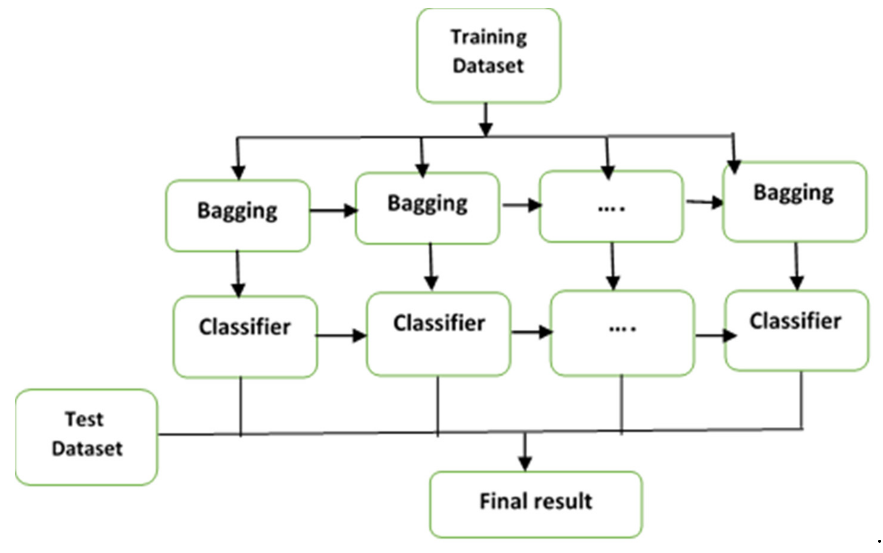
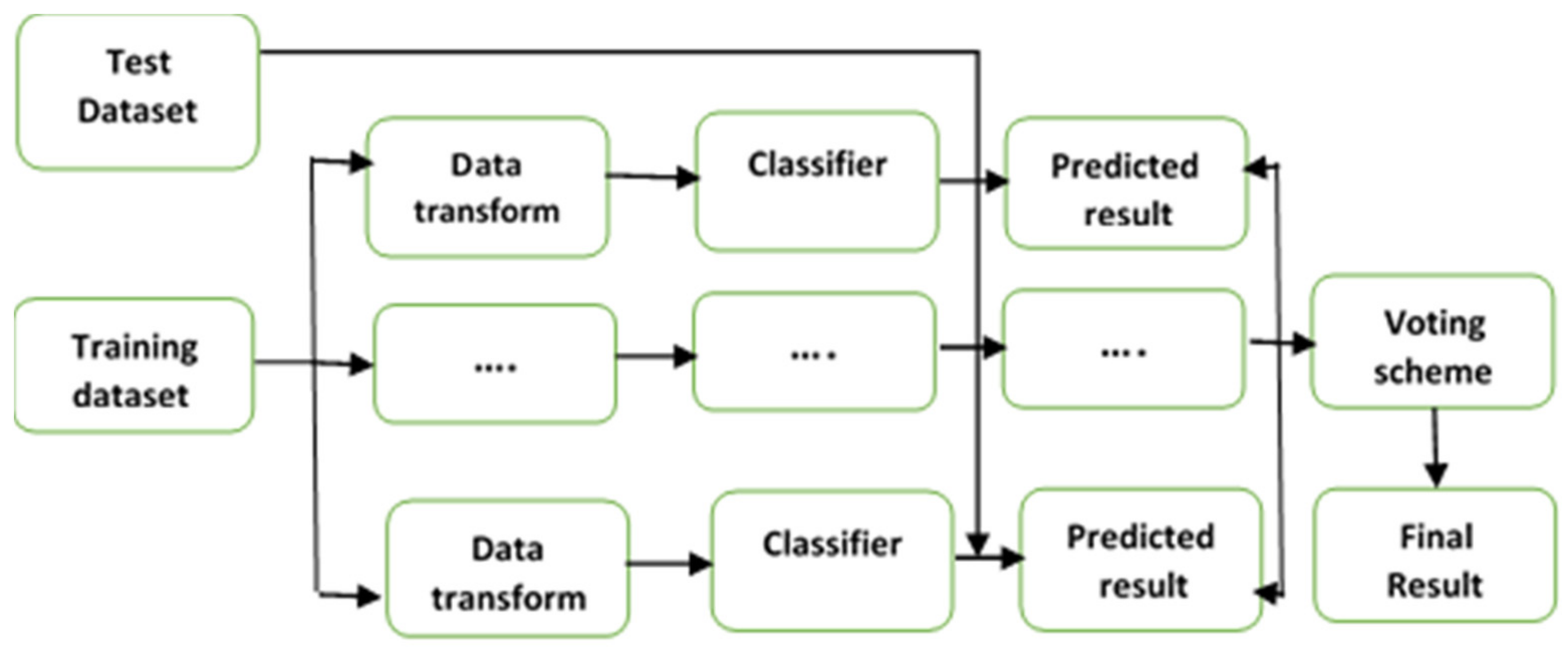
3.1. Ensemble Classification
3.2. Hyperparameter Optimization
3.3. Minimum Redundancy Maximum Relevance (mRMR) for Feature Selection
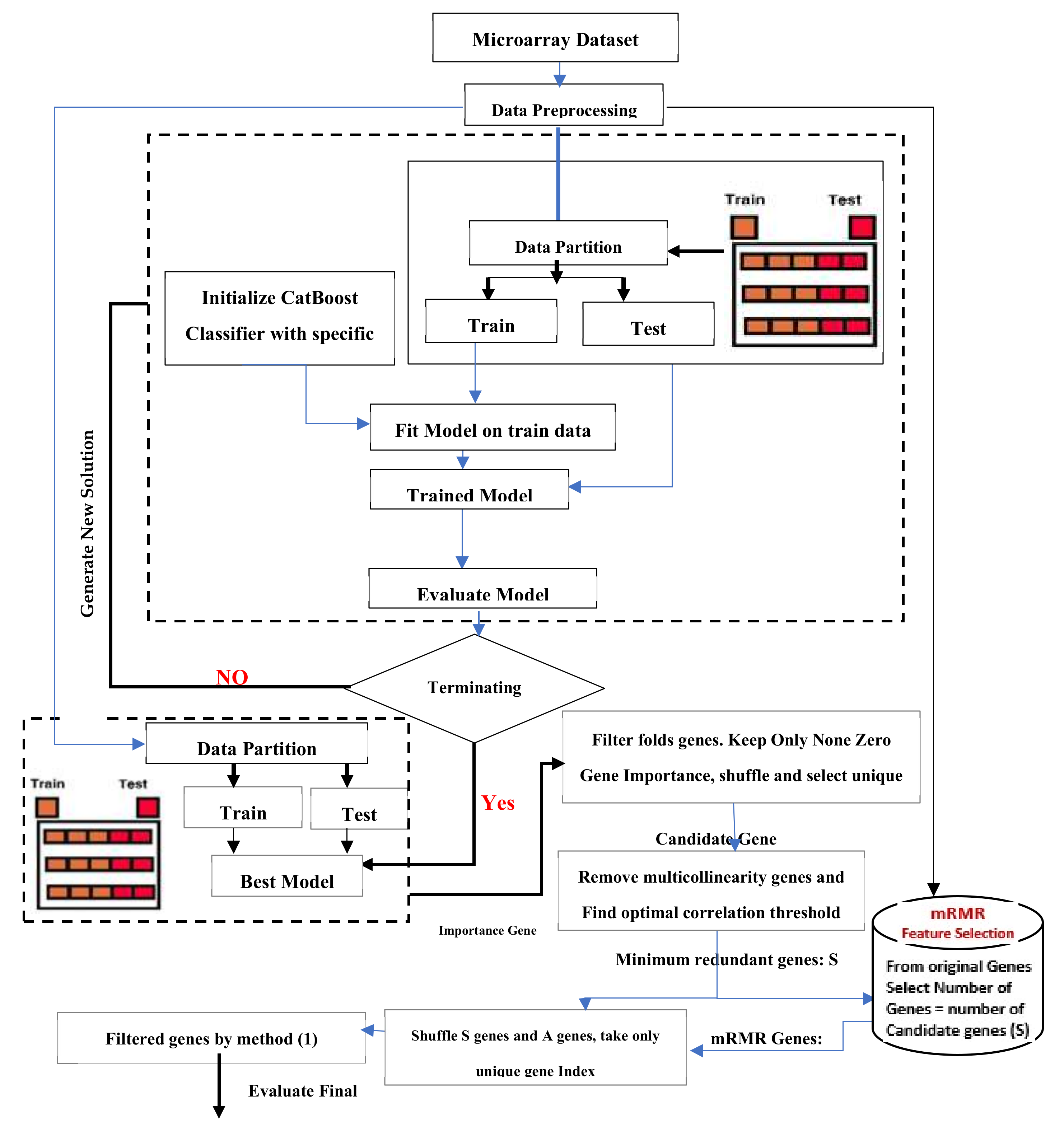
4. The Proposed Hybrid Model
- (i)
- Preprocessing the dataset (brain cancer microarray). This step is vital to
- Avoid features in greater numeric ranges dominating those in smaller ranges;
- Avoid numerical difficulties during calculation;
- Ensure that each feature is scaled to the range [0, 1].
- (ii)
- The data were partitioned into two sets: The training set is used for the training. The testing set is used to test final model 3, initializing CatBoost with specific solution parameters. Table 3 describes the parameter initialization of the classifiers
- (iii)
- CatBoost is used as a feature selector with 8-fold cross-validations (8 cross-validations of different levels of importance for every gene index). CatBoost calculates the means for each fold.
- (iv)
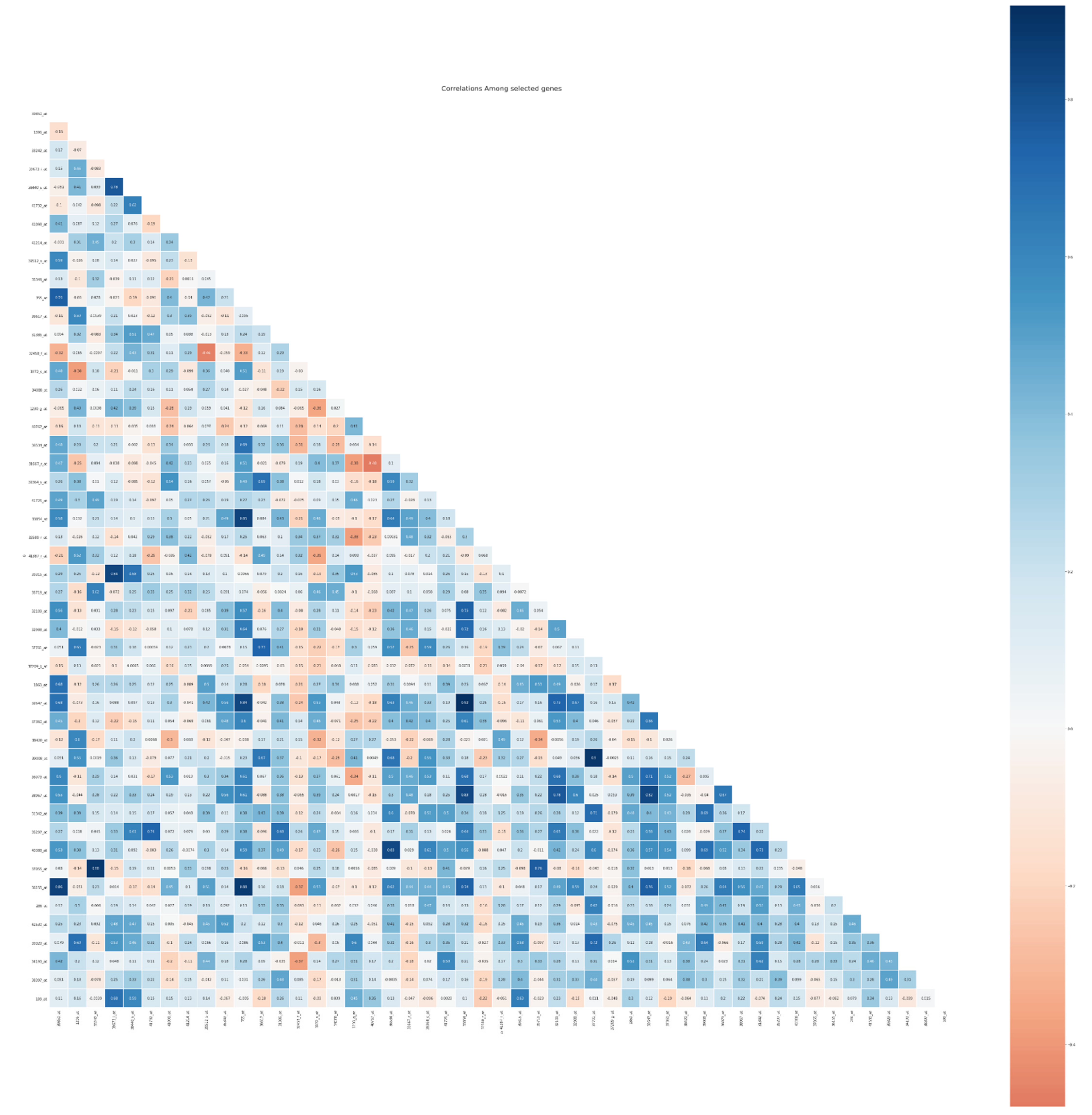
- By setting a threshold, irrelevant features are then removed. Suppose the score of a gene is above the threshold. In that case, the gene will be selected (as seen in Appendix A, the optimal threshold that offers the maximum accuracy is: 0.84). The genes are shuffled, and unique genes are kept.
- (v)
- The importance value of each gene is registered using a voting process. For example, the gene with index 1 in fold 0 receives an importance value of 1 if the same gene is present in the next fold; then, the gene importance is +1, and so on, for all of the 8-fold cross-validations. After this was applied, voting is conducted 50 genes (six of the filtered genes are genes with an importance >8.
5. Results and Discussion
5.1. Datasets
5.2. Experiment 1: Comparing Performance of Optimized (CatBoost and XGBoost) with the Proposed Hybrid Model
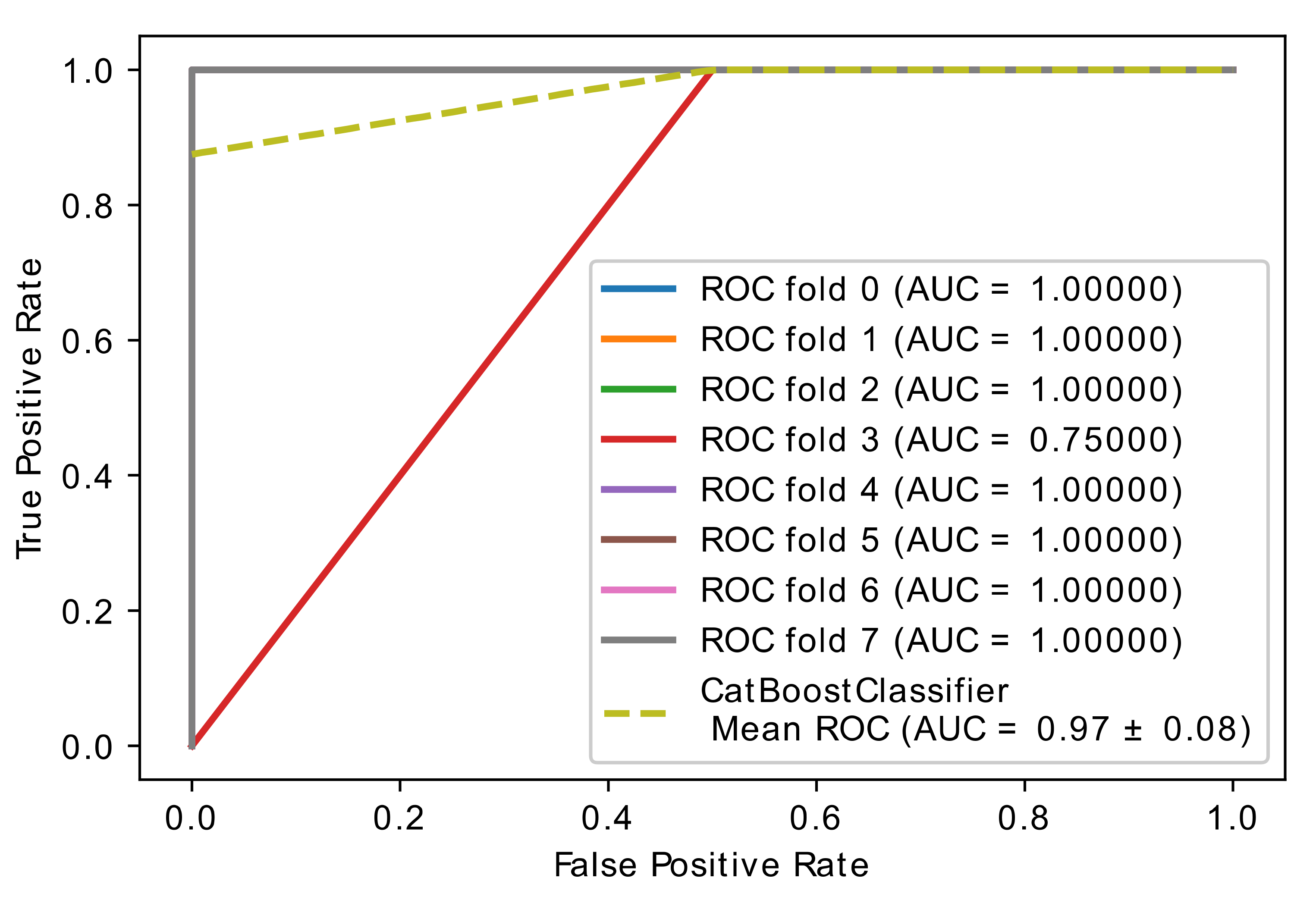
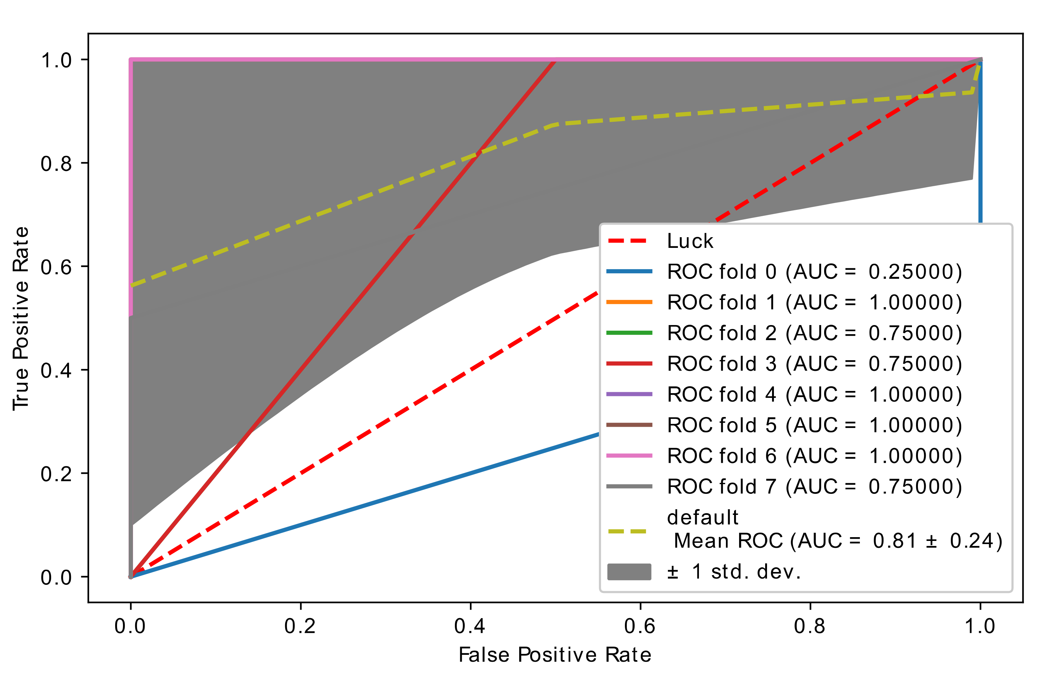
5.3. Experiment 2: Comparing Performance of CatBoost and Optimized CatBoost Classifier
- Number of non-zero genes importance (every fold).
- (588, 576, 590, 599, 594, 579, 585, 584).
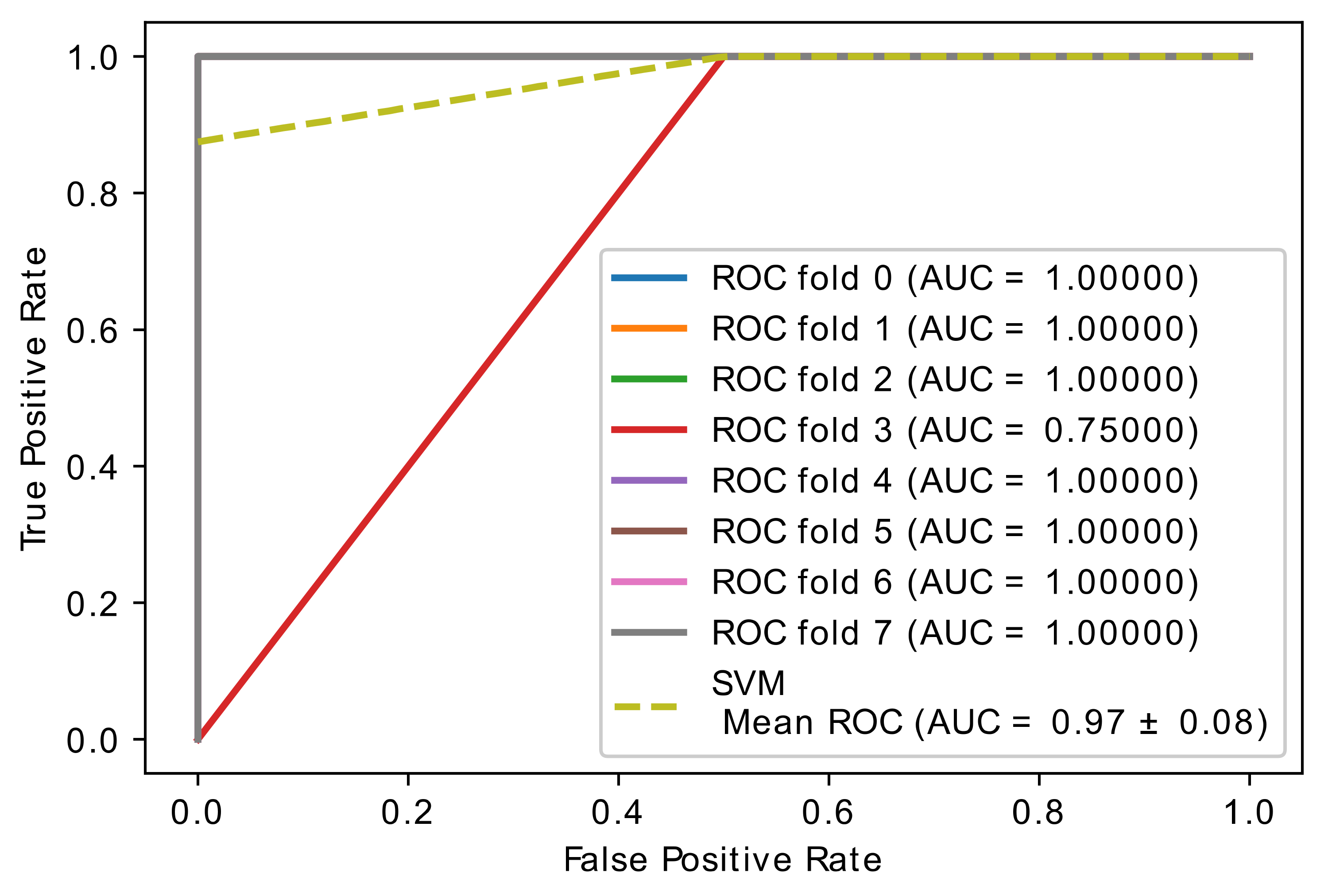
- The number of genes selected by embedded SVM (with Redundant), 980 genes.
- The number of genes selected by embedded SVM (Unique), 671 genes.
- The final number of genes after we applied voting was 50 genes.
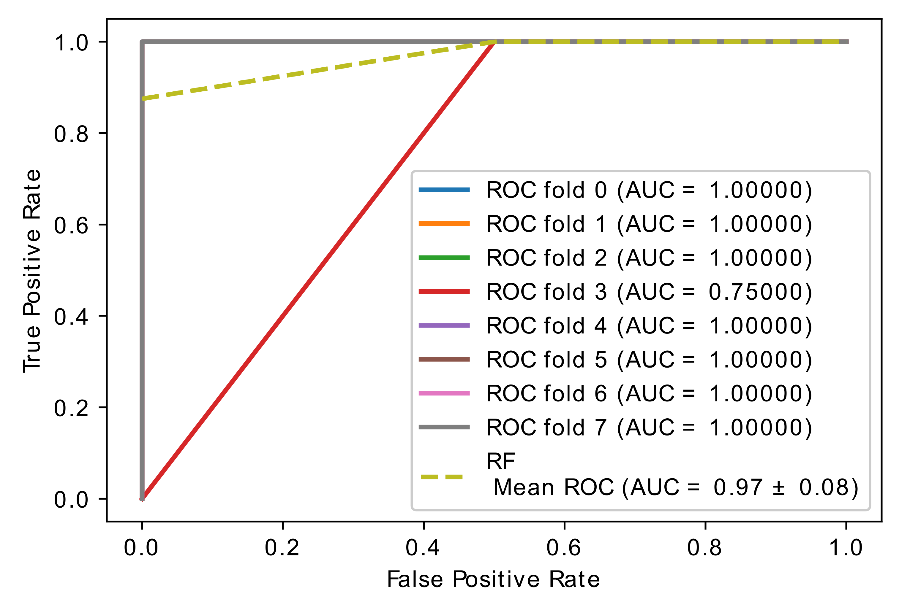
5.4. Experiment 3: Comparison of Hybrid Proposed Model Performance by Different Classification
5.5. Biological Interpretation
6. Conclusions
Author Contributions
Funding
Institutional Review Board Statement
Informed Consent Statement
Data Availability Statement
Conflicts of Interest
Appendix A

| Threshold (28: 1068) | SVM | Random Forest | Naive Bayes | CatBoost | ||||||||||||
|---|---|---|---|---|---|---|---|---|---|---|---|---|---|---|---|---|
| Accuracy | Spec | SEN | AUC | Accuracy | Spec | SEN | AUC | Accuracy | Spec | SEN | AUC | Accuracy | Spec | SEN | AUC | |
| 0.5 | 0.91 ± 0.17 | 1.00 ± 0.00 | 0.81 ± 0.35 | 0.91 ± 0.17 | 0.97 ± 0.08 | 1.00 ± 0.00 | 0.94 ± 0.17 | 0.97 ± 0.08 | 1.00 ± 0.00 | 1.00 ± 0.00 | 1.00 ± 0.00 | 1.00 ± 0.00 | 0.91 ± 0.12 | 0.94 ± 0.17 | 0.88 ± 0.22 | 0.91 ± 0.12 |
| 0.51 | 0.91 ± 0.17 | 1.00 ± 0.00 | 0.81 ± 0.35 | 0.91 ± 0.17 | 0.97 ± 0.08 | 0.94 ± 0.17 | 1.00 ± 0.00 | 0.97 ± 0.08 | 1.00 ± 0.00 | 1.00 ± 0.00 | 1.00 ± 0.00 | 1.00 ± 0.00 | 0.91 ± 0.12 | 0.94 ± 0.17 | 0.88 ± 0.22 | 0.91 ± 0.12 |
| 0.52 | 0.91 ± 0.17 | 1.00 ± 0.00 | 0.81 ± 0.35 | 0.91 ± 0.17 | 0.91 ± 0.17 | 0.88 ± 0.33 | 0.94 ± 0.17 | 0.91 ± 0.17 | 1.00 ± 0.00 | 1.00 ± 0.00 | 1.00 ± 0.00 | 1.00 ± 0.00 | 0.91 ± 0.12 | 0.94 ± 0.17 | 0.88 ± 0.22 | 0.91 ± 0.12 |
| 0.53 | 0.91 ± 0.17 | 1.00 ± 0.00 | 0.81 ± 0.35 | 0.91 ± 0.17 | 0.94 ± 0.11 | 1.00 ± 0.00 | 0.88 ± 0.22 | 0.94 ± 0.11 | 1.00 ± 0.00 | 1.00 ± 0.00 | 1.00 ± 0.00 | 1.00 ± 0.00 | 0.91 ± 0.12 | 0.94 ± 0.17 | 0.88 ± 0.22 | 0.91 ± 0.12 |
| 0.54 | 0.91 ± 0.17 | 1.00 ± 0.00 | 0.81 ± 0.35 | 0.91 ± 0.17 | 0.97 ± 0.08 | 1.00 ± 0.00 | 0.94 ± 0.17 | 0.97 ± 0.08 | 1.00 ± 0.00 | 1.00 ± 0.00 | 1.00 ± 0.00 | 1.00 ± 0.00 | 0.91 ± 0.12 | 0.94 ± 0.17 | 0.88 ± 0.22 | 0.91 ± 0.12 |
| 0.55 | 0.91 ± 0.17 | 1.00 ± 0.00 | 0.81 ± 0.35 | 0.91 ± 0.17 | 0.93 ± 0.13 | 1.00 ± 0.00 | 0.88 ± 0.22 | 0.94 ± 0.11 | 1.00 ± 0.00 | 1.00 ± 0.00 | 1.00 ± 0.00 | 1.00 ± 0.00 | 0.91 ± 0.12 | 0.94 ± 0.17 | 0.88 ± 0.22 | 0.91 ± 0.12 |
| 0.56 | 0.91 ± 0.17 | 1.00 ± 0.00 | 0.81 ± 0.35 | 0.91 ± 0.17 | 0.97 ± 0.08 | 1.00 ± 0.00 | 0.94 ± 0.17 | 0.97 ± 0.08 | 1.00 ± 0.00 | 1.00 ± 0.00 | 1.00 ± 0.00 | 1.00 ± 0.00 | 0.91 ± 0.12 | 0.94 ± 0.17 | 0.88 ± 0.22 | 0.91 ± 0.12 |
| 0.57 | 0.91 ± 0.17 | 1.00 ± 0.00 | 0.81 ± 0.35 | 0.91 ± 0.17 | 0.94 ± 0.11 | 0.94 ± 0.17 | 0.94 ± 0.17 | 0.94 ± 0.11 | 1.00 ± 0.00 | 1.00 ± 0.00 | 1.00 ± 0.00 | 1.00 ± 0.00 | 0.91 ± 0.12 | 0.94 ± 0.17 | 0.88 ± 0.22 | 0.91 ± 0.12 |
| 0.58 | 0.93 ± 0.13 | 1.00 ± 0.00 | 0.88 ± 0.22 | 0.94 ± 0.11 | 0.88 ± 0.12 | 0.94 ± 0.17 | 0.81 ± 0.24 | 0.88 ± 0.12 | 0.97 ± 0.08 | 0.94 ± 0.17 | 1.00 ± 0.00 | 0.97 ± 0.08 | 0.91 ± 0.12 | 0.94 ± 0.17 | 0.88 ± 0.22 | 0.91 ± 0.12 |
| 0.59 | 0.97 ± 0.08 | 1.00 ± 0.00 | 0.94 ± 0.17 | 0.97 ± 0.08 | 0.91 ± 0.12 | 0.94 ± 0.17 | 0.88 ± 0.22 | 0.91 ± 0.12 | 1.00 ± 0.00 | 1.00 ± 0.00 | 1.00 ± 0.00 | 1.00 ± 0.00 | 0.91 ± 0.12 | 0.94 ± 0.17 | 0.88 ± 0.22 | 0.91 ± 0.12 |
| 0.6 | 0.97 ± 0.08 | 1.00 ± 0.00 | 0.94 ± 0.17 | 0.97 ± 0.08 | 0.91 ± 0.12 | 0.94 ± 0.17 | 0.88 ± 0.22 | 0.91 ± 0.12 | 1.00 ± 0.00 | 1.00 ± 0.00 | 1.00 ± 0.00 | 1.00 ± 0.00 | 0.91 ± 0.12 | 0.94 ± 0.17 | 0.88 ± 0.22 | 0.91 ± 0.12 |
| 0.61 | 0.97 ± 0.08 | 1.00 ± 0.00 | 0.94 ± 0.17 | 0.97 ± 0.08 | 0.86 ± 0.19 | 0.88 ± 0.22 | 0.88 ± 0.22 | 0.88 ± 0.18 | 0.97 ± 0.08 | 0.94 ± 0.17 | 1.00 ± 0.00 | 0.97 ± 0.08 | 0.90 ± 0.14 | 1.00 ± 0.00 | 0.81 ± 0.24 | 0.91 ± 0.12 |
| 0.62 | 0.97 ± 0.08 | 1.00 ± 0.00 | 0.94 ± 0.17 | 0.97 ± 0.08 | 0.90 ± 0.14 | 0.94 ± 0.17 | 0.88 ± 0.22 | 0.91 ± 0.12 | 0.97 ± 0.08 | 0.94 ± 0.17 | 1.00 ± 0.00 | 0.97 ± 0.08 | 0.90 ± 0.14 | 1.00 ± 0.00 | 0.81 ± 0.24 | 0.91 ± 0.12 |
| 0.63 | 0.97 ± 0.08 | 1.00 ± 0.00 | 0.94 ± 0.17 | 0.97 ± 0.08 | 0.83 ± 0.18 | 0.88 ± 0.22 | 0.81 ± 0.24 | 0.84 ± 0.17 | 0.97 ± 0.08 | 0.94 ± 0.17 | 1.00 ± 0.00 | 0.97 ± 0.08 | 0.94 ± 0.11 | 1.00 ± 0.00 | 0.88 ± 0.22 | 0.94 ± 0.11 |
| 0.64 | 0.97 ± 0.08 | 1.00 ± 0.00 | 0.94 ± 0.17 | 0.97 ± 0.08 | 0.97 ± 0.08 | 1.00 ± 0.00 | 0.94 ± 0.17 | 0.97 ± 0.08 | 0.97 ± 0.08 | 1.00 ± 0.00 | 0.94 ± 0.17 | 0.97 ± 0.08 | 0.94 ± 0.11 | 1.00 ± 0.00 | 0.88 ± 0.22 | 0.94 ± 0.11 |
| 0.65 | 0.94± 0.11 | 1.00 ± 0.00 | 0.88 ± 0.22 | 0.94 ± 0.11 | 0.97 ± 0.08 | 1.00 ± 0.00 | 0.94 ± 0.17 | 0.97 ± 0.08 | 1.00 ± 0.00 | 1.00 ± 0.00 | 1.00 ± 0.00 | 1.00 ± 0.00 | 0.91 ± 0.12 | 0.94 ± 0.17 | 0.88 ± 0.22 | 0.91 ± 0.12 |
| 0.66 | 0.97 ± 0.08 | 1.00 ± 0.00 | 0.94 ± 0.17 | 0.97 ± 0.08 | 0.97 ± 0.08 | 1.00 ± 0.00 | 0.94 ± 0.17 | 0.97 ± 0.08 | 0.97 ± 0.08 | 0.94 ± 0.17 | 1.00 ± 0.00 | 0.97 ± 0.08 | 0.94 ± 0.11 | 1.00 ± 0.00 | 0.88 ± 0.22 | 0.94 ± 0.11 |
| 0.67 | 0.97 ± 0.08 | 1.00 ± 0.00 | 0.94 ± 0.17 | 0.97 ± 0.08 | 0.94 ± 0.17 | 0.94 ± 0.17 | 0.94 ± 0.17 | 0.94 ± 0.17 | 0.97 ± 0.08 | 0.94 ± 0.17 | 1.00 ± 0.00 | 0.97 ± 0.08 | 0.94 ± 0.17 | 1.00 ± 0.00 | 0.97 ± 0.08 | 0.94 ± 0.11 |
| 0.68 | 0.97 ± 0.08 | 1.00 ± 0.00 | 0.94 ± 0.17 | 0.97 ± 0.08 | 0.94 ± 0.17 | 0.94 ± 0.17 | 0.94 ± 0.17 | 0.94 ± 0.17 | 0.97 ± 0.08 | 0.94 ± 0.17 | 1.00 ± 0.00 | 0.97 ± 0.08 | 0.94 ± 0.11 | 1.00 ± 0.00 | 0.88 ± 0.22 | 0.94 ± 0.11 |
| 0.69 | 0.97 ± 0.08 | 1.00 ± 0.00 | 0.94 ± 0.17 | 0.97 ± 0.08 | 0.91 ± 0.17 | 0.94 ± 0.17 | 0.88 ± 0.22 | 0.91 ± 0.17 | 0.97 ± 0.08 | 0.94 ± 0.17 | 1.00 ± 0.00 | 0.97 ± 0.08 | 0.94 ± 0.11 | 1.00 ± 0.00 | 0.88 ± 0.22 | 0.94 ± 0.11 |
| 0.7 | 0.94 ± 0.11 | 1.00 ± 0.00 | 0.88 ± 0.22 | 0.94 ± 0.11 | 0.91 ± 0.17 | 0.94 ± 0.17 | 0.88 ± 0.22 | 0.91 ± 0.17 | 0.91 ± 0.12 | 0.81 ± 0.24 | 1.00 ± 0.00 | 0.91 ± 0.12 | 0.94 ± 0.11 | 1.00 ± 0.00 | 0.88 ± 0.22 | 0.94 ± 0.11 |
| 0.71 | 0.94 ± 0.11 | 1.00 ± 0.00 | 0.88 ± 0.22 | 0.94 ± 0.11 | 0.91 ± 0.17 | 0.94 ± 0.17 | 0.88 ± 0.22 | 0.91 ± 0.17 | 0.93 ± 0.13 | 0.88 ± 0.22 | 1.00 ± 0.00 | 0.94 ± 0.11 | 0.91 ± 0.12 | 0.94 ± 0.17 | 0.81 ± 0.24 | 0.91 ± 0.12 |
| 0.72 | 0.94 ± 0.11 | 1.00 ± 0.00 | 0.88 ± 0.22 | 0.94 ± 0.11 | 0.97 ± 0.08 | 1.00 ± 0.00 | 0.94 ± 0.17 | 0.97 ± 0.08 | 0.90 ± 0.14 | 0.88 ± 0.22 | 0.94 ± 0.17 | 0.91 ± 0.12 | 0.91 ± 0.12 | 1.00 ± 0.00 | 0.81 ± 0.24 | 0.91 ± 0.12 |
| 0.73 | 0.94 ± 0.11 | 1.00 ± 0.00 | 0.88 ± 0.22 | 0.94 ± 0.11 | 0.94 ± 0.17 | 0.94 ± 0.17 | 0.94 ± 0.17 | 0.94 ± 0.17 | 0.90 ± 0.14 | 0.88 ± 0.22 | 0.94 ± 0.17 | 0.91 ± 0.12 | 0.91 ± 0.12 | 1.00 ± 0.00 | 0.81 ± 0.24 | 0.91 ± 0.12 |
| 0.74 | 0.97 ± 0.08 | 1.00 ± 0.00 | 0.94 ± 0.17 | 0.97 ± 0.08 | 0.91 ± 0.17 | 0.94 ± 0.17 | 0.88 ± 0.22 | 0.91 ± 0.17 | 0.93 ± 0.13 | 0.88 ± 0.22 | 1.00 ± 0.00 | 0.94 ± 0.11 | 0.94 ± 0.11 | 1.00 ± 0.00 | 0.88 ± 0.22 | 0.94 ± 0.11 |
| 0.75 | 0.97 ± 0.08 | 1.00 ± 0.00 | 0.94 ± 0.17 | 0.97 ± 0.08 | 0.97 ± 0.08 | 1.00 ± 0.00 | 0.94 ± 0.17 | 0.97 ± 0.08 | 0.90 ± 0.14 | 0.88 ± 0.22 | 0.94 ± 0.17 | 0.91 ± 0.12 | 0.94 ± 0.11 | 1.00 ± 0.00 | 0.88 ± 0.22 | 0.94 ± 0.11 |
| 0.76 | 0.97 ± 0.08 | 1.00 ± 0.00 | 0.94 ± 0.17 | 0.97 ± 0.08 | 0.94 ± 0.17 | 0.94 ± 0.17 | 0.94 ± 0.17 | 0.94 ± 0.17 | 0.80 ± 0.21 | 0.75 ± 0.35 | 0.88 ± 0.22 | 0.81 ± 0.21 | 0.94 ± 0.11 | 1.00 ± 0.00 | 0.88 ± 0.22 | 0.94 ± 0.11 |
| 0.77 | 0.97 ± 0.08 | 1.00 ± 0.00 | 0.94 ± 0.17 | 0.97 ± 0.08 | 0.93 ± 0.13 | 0.94 ± 0.17 | 0.94 ± 0.17 | 0.94 ± 0.11 | 0.80 ± 0.21 | 0.75 ± 0.35 | 0.88 ± 0.22 | 0.81 ± 0.21 | 0.94 ± 0.11 | 1.00 ± 0.00 | 0.88 ± 0.22 | 0.94 ± 0.11 |
| 0.78 | 0.97 ± 0.08 | 1.00 ± 0.00 | 0.94 ± 0.17 | 0.97 ± 0.08 | 0.86 ± 0.19 | 0.88 ± 0.22 | 0.88 ± 0.22 | 0.88 ± 0.18 | 0.83 ± 0.18 | 0.75 ± 0.35 | 0.94 ± 0.17 | 0.84 ± 0.17 | 0.94 ± 0.11 | 1.00 ± 0.00 | 0.88 ± 0.22 | 0.94 ± 0.11 |
| 0.79 | 1.00 ± 0.00 | 1.00 ± 0.00 | 1.00 ± 0.00 | 1.00 ± 0.00 | 0.90 ± 0.19 | 0.88 ± 0.22 | 0.94 ± 0.17 | 0.91 ± 0.17 | 0.83 ± 0.18 | 0.75 ± 0.35 | 0.94 ± 0.17 | 0.84 ± 0.17 | 0.94 ± 0.11 | 1.00 ± 0.00 | 0.88 ± 0.22 | 0.94 ± 0.11 |
| 0.8 | 1.00 ± 0.00 | 1.00 ± 0.00 | 1.00 ± 0.00 | 1.00 ± 0.00 | 0.94 ± 0.11 | 1.00 ± 0.00 | 0.88 ± 0.22 | 0.94 ± 0.11 | 0.86 ± 0.14 | 0.75 ± 0.35 | 0.94 ± 0.17 | 0.84 ± 0.17 | 0.94 ± 0.11 | 1.00 ± 0.00 | 0.88 ± 0.22 | 0.94 ± 0.11 |
| 0.81 | 1.00 ± 0.00 | 1.00 ± 0.00 | 1.00 ± 0.00 | 1.00 ± 0.00 | 0.97 ± 0.08 | 1.00 ± 0.00 | 0.94 ± 0.17 | 0.97 ± 0.08 | 0.83 ± 0.19 | 0.81 ± 0.24 | 0.94 ± 0.17 | 0.88 ± 0.18 | 0.90 ± 0.14 | 0.94 ± 0.17 | 0.88 ± 0.22 | 0.91 ± 0.12 |
| 0.82 | 1.00 ± 0.00 | 1.00 ± 0.00 | 1.00 ± 0.00 | 1.00 ± 0.00 | 0.93 ± 0.13 | 0.94 ± 0.17 | 0.94 ± 0.17 | 0.94 ± 0.11 | 0.86 ± 0.19 | 0.81 ± 0.24 | 0.94 ± 0.17 | 0.88 ± 0.18 | 0.90 ± 0.14 | 0.94 ± 0.17 | 0.88 ± 0.22 | 0.91 ± 0.12 |
| 0.83 | 1.00 ± 0.00 | 1.00 ± 0.00 | 1.00 ± 0.00 | 1.00 ± 0.00 | 0.97 ± 0.08 | 1.00 ± 0.00 | 0.94 ± 0.17 | 0.97 ± 0.08 | 0.90 ± 0.14 | 0.81 ± 0.24 | 1.00 ± 0.00 | 0.91 ± 0.12 | 0.93 ± 0.13 | 0.94 ± 0.17 | 0.94 ± 0.17 | 0.94 ± 0.11 |
| 0.84 | 1.00 ± 0.00 | 1.00 ± 0.00 | 1.00 ± 0.00 | 1.00 ± 0.00 | 0.97 ± 0.08 | 1.00 ± 0.00 | 0.94 ± 0.17 | 0.97 ± 0.08 | 0.90 ± 0.14 | 0.81 ± 0.24 | 1.00 ± 0.00 | 0.91 ± 0.12 | 0.97 ± 0.08 | 1.00 ± 0.00 | 0.94 ± 0.17 | 0.97 ± 0.08 |
| 0.85 | 0.97 ± 0.08 | 1.00 ± 0.00 | 0.94 ± 0.17 | 0.97 ± 0.08 | 0.93 ± 0.13 | 0.94 ± 0.17 | 0.94 ± 0.17 | 0.94 ± 0.11 | 0.90 ± 0.14 | 0.81 ± 0.24 | 1.00 ± 0.00 | 0.91 ± 0.12 | 0.97 ± 0.08 | 1.00 ± 0.00 | 0.94 ± 0.17 | 0.97 ± 0.08 |
| 0.86 | 0.97 ± 0.08 | 1.00 ± 0.00 | 0.94 ± 0.17 | 0.97 ± 0.08 | 0.97 ± 0.08 | 1.00 ± 0.00 | 0.94 ± 0.17 | 0.97 ± 0.08 | 0.90 ± 0.14 | 0.81 ± 0.24 | 1.00 ± 0.00 | 0.91 ± 0.12 | 0.93 ± 0.13 | 0.94 ± 0.17 | 0.94 ± 0.17 | 0.94 ± 0.11 |
| 0.87 | 0.97 ± 0.08 | 1.00 ± 0.00 | 0.94 ± 0.17 | 0.97 ± 0.08 | 0.97 ± 0.08 | 1.00 ± 0.00 | 0.94 ± 0.17 | 0.97 ± 0.08 | 0.90 ± 0.14 | 0.81 ± 0.24 | 1.00 ± 0.00 | 0.91 ± 0.12 | 0.93 ± 0.13 | 0.94 ± 0.17 | 0.94 ± 0.17 | 0.94 ± 0.11 |
| 0.88 | 0.97 ± 0.08 | 1.00 ± 0.00 | 0.94 ± 0.17 | 0.97 ± 0.08 | 0.97 ± 0.08 | 1.00 ± 0.00 | 0.94 ± 0.17 | 0.97 ± 0.08 | 0.90 ± 0.14 | 0.81 ± 0.24 | 1.00 ± 0.00 | 0.91 ± 0.12 | 0.93 ± 0.13 | 0.94 ± 0.17 | 0.94 ± 0.17 | 0.94 ± 0.11 |
| 0.89 | 0.97 ± 0.08 | 1.00 ± 0.00 | 0.94 ± 0.17 | 0.97 ± 0.08 | 0.94 ± 0.11 | 1.00 ± 0.00 | 0.88 ± 0.22 | 0.94 ± 0.11 | 0.90 ± 0.14 | 0.81 ± 0.24 | 1.00 ± 0.00 | 0.91 ± 0.12 | 0.97 ± 0.08 | 1.00 ± 0.00 | 0.94 ± 0.17 | 0.97 ± 0.08 |
| 0.9 | 0.97 ± 0.08 | 1.00 ± 0.00 | 0.94 ± 0.17 | 0.97 ± 0.08 | 0.93 ± 0.13 | 0.94 ± 0.17 | 0.94 ± 0.17 | 0.94 ± 0.11 | 0.90 ± 0.14 | 0.81 ± 0.24 | 1.00 ± 0.00 | 0.91 ± 0.12 | 0.97 ± 0.08 | 1.00 ± 0.00 | 0.94 ± 0.17 | 0.97 ± 0.08 |
| 0.91 | 0.97 ± 0.08 | 1.00 ± 0.00 | 0.94 ± 0.17 | 0.97 ± 0.08 | 0.90 ± 0.14 | 0.81 ± 0.24 | 1.00 ± 0.00 | 0.91 ± 0.12 | 0.90 ± 0.14 | 0.81 ± 0.24 | 1.00 ± 0.00 | 0.91 ± 0.12 | 0.97 ± 0.08 | 1.00 ± 0.00 | 0.94 ± 0.17 | 0.97 ± 0.08 |
| 0.92 | 0.97 ± 0.08 | 1.00 ± 0.00 | 0.94 ± 0.17 | 0.97 ± 0.08 | 0.93 ± 0.13 | 0.94 ± 0.17 | 0.94 ± 0.17 | 0.94 ± 0.11 | 0.83 ± 0.18 | 0.69 ± 0.35 | 1.00 ± 0.00 | 0.84 ± 0.17 | 0.97 ± 0.08 | 1.00 ± 0.00 | 0.94 ± 0.17 | 0.97 ± 0.08 |
| 0.93 | 0.97 ± 0.08 | 1.00 ± 0.00 | 0.94 ± 0.17 | 0.97 ± 0.08 | 0.90 ± 0.14 | 0.94 ± 0.17 | 0.88 ± 0.22 | 0.91 ± 0.12 | 0.83 ± 0.18 | 0.69 ± 0.35 | 1.00 ± 0.00 | 0.84 ± 0.17 | 0.97 ± 0.08 | 1.00 ± 0.00 | 0.94 ± 0.17 | 0.97 ± 0.08 |
| 0.94 | 0.97 ± 0.08 | 1.00 ± 0.00 | 0.94 ± 0.17 | 0.97 ± 0.08 | 0.93 ± 0.13 | 0.94 ± 0.17 | 0.94 ± 0.17 | 0.94 ± 0.11 | 0.83 ± 0.18 | 0.69 ± 0.35 | 1.00 ± 0.00 | 0.84 ± 0.17 | 0.97 ± 0.08 | 1.00 ± 0.00 | 0.94 ± 0.17 | 0.97 ± 0.08 |
| 0.95 | 0.97 ± 0.08 | 1.00 ± 0.00 | 0.94 ± 0.17 | 0.97 ± 0.08 | 0.97 ± 0.08 | 1.00 ± 0.00 | 0.94 ± 0.17 | 0.97 ± 0.08 | 0.83 ± 0.18 | 0.69 ± 0.35 | 1.00 ± 0.00 | 0.84 ± 0.17 | 0.97 ± 0.08 | 1.00 ± 0.00 | 0.94 ± 0.17 | 0.97 ± 0.08 |
| 0.96 | 0.97 ± 0.08 | 1.00 ± 0.00 | 0.94 ± 0.17 | 0.97 ± 0.08 | 0.97 ± 0.08 | 1.00 ± 0.00 | 0.94 ± 0.17 | 0.97 ± 0.08 | 0.83 ± 0.18 | 0.69 ± 0.35 | 1.00 ± 0.00 | 0.84 ± 0.17 | 0.93 ± 0.13 | 0.94 ± 0.17 | 0.94 ± 0.17 | 0.94 ± 0.11 |
| 0.97 | 0.94 ± 0.11 | 0.94 ± 0.17 | 0.94 ± 0.17 | 0.94 ± 0.11 | 0.93 ± 0.13 | 0.94 ± 0.17 | 0.94 ± 0.17 | 0.94 ± 0.11 | 0.83 ± 0.18 | 0.69 ± 0.35 | 1.00 ± 0.00 | 0.84 ± 0.17 | 0.97 ± 0.08 | 1.00 ± 0.00 | 0.94 ± 0.17 | 0.97 ± 0.08 |
| 0.98 | 0.94 ± 0.11 | 0.94 ± 0.17 | 0.94 ± 0.17 | 0.94 ± 0.11 | 0.97 ± 0.08 | 1.00 ± 0.00 | 0.94 ± 0.17 | 0.97 ± 0.08 | 0.83 ± 0.18 | 0.69 ± 0.35 | 1.00 ± 0.00 | 0.84 ± 0.17 | 0.97 ± 0.08 | 1.00 ± 0.00 | 0.94 ± 0.17 | 0.97 ± 0.08 |
| 0.99 | 0.94 ± 0.11 | 0.94 ± 0.17 | 0.94 ± 0.17 | 0.94 ± 0.11 | 0.97 ± 0.08 | 1.00 ± 0.00 | 0.94 ± 0.17 | 0.97 ± 0.08 | 0.83 ± 0.18 | 0.69 ± 0.35 | 1.00 ± 0.00 | 0.84 ± 0.17 | 0.97 ± 0.08 | 1.00 ± 0.00 | 0.94 ± 0.17 | 0.97 ± 0.08 |
References
- Siegel, R.L.; Miller, K.D.; Jemal, A. Cancer statistics, 2021. CA A Cancer J. Clin. 2021, 66, 7–30. [Google Scholar] [CrossRef] [PubMed] [Green Version]
- Rehman, M.U.; Cho, S.; Kim, J.; Chong, K.T. BrainSeg-Net: Brain Tumor MR Image Segmentation via Enhanced Encoder–Decoder Network. Diagnostics 2021, 11, 169. [Google Scholar] [CrossRef]
- Havaei, M.; Davy, A.; Warde-Farley, D.; Biard, A.; Courville, A.; Bengio, Y.; Pal, C.; Jodoin, P.-M.; Larochelle, H. Brain tumor segmentation with Deep Neural Networks. Med. Image Anal. 2017, 35, 18–31. [Google Scholar] [CrossRef] [PubMed] [Green Version]
- Isensee, F.; Jäger, P.F.; Full, P.M.; Vollmuth, P.; Maier-Hein, K.H. nnU-net for brain tumor segmentation. In International MICCAI Brainlesion Workshop; Springer: Cham, Switzerland, 2020; pp. 118–132. [Google Scholar]
- Zeineldin, R.A.; Karar, M.E.; Coburger, J.; Wirtz, C.R.; Burgert, O. DeepSeg: Deep neural network framework for automatic brain tumor segmentation using magnetic resonance FLAIR images. Int. J. Comput. Assist. Radiol. Surg. 2020, 15, 909–920. [Google Scholar] [CrossRef]
- Perrin, S.L.; Samuel, M.S.; Koszyca, B.; Brown, M.P.; Ebert, L.M.; Oksdath, M.; Gomez, G.A. Glioblastoma heterogeneity and the tumour microenvironment: Implications for preclinical research and development of new treatments. Biochem. Soc. Trans. 2019, 47, 625–638. [Google Scholar] [CrossRef]
- Golub, T.R.; Slonim, D.K.; Tamayo, P.; Huard, C.; Gaasenbeek, M.; Mesirov, J.P.; Coller, H.; Loh, M.L.; Downing, J.R.; Caligiuri, M.A.; et al. Molecular Classification of Cancer: Class Discovery and Class Prediction by Gene Expression Monitoring. Science 1999, 286, 531–537. [Google Scholar] [CrossRef] [Green Version]
- Leung, Y.F.; Cavalieri, D. Fundamentals of cDNA microarray data analysis. Trends Genet. 2003, 19, 649–659. [Google Scholar] [CrossRef] [PubMed]
- Flores, M.; Hsiao, T.-H.; Chiu, Y.-C.; Chuang, E.Y.; Huang, Y.; Chen, Y. Gene Regulation, Modulation, and Their Applications in Gene Expression Data Analysis. Adv. Bioinform. 2013, 2013, 1–11. [Google Scholar] [CrossRef] [PubMed] [Green Version]
- Friedman, J.H. Stochastic gradient boosting. Comput. Stat. Data Anal. 2002, 38, 367–378. [Google Scholar] [CrossRef]
- Bergstra, J.; Komer, B.; Eliasmith, C.; Yamins, D.; Cox, D. Hyperopt: A Python library for model selection and hyperparameter optimization. Comput. Sci. Discov. 2015, 8, 014008. [Google Scholar] [CrossRef]
- De Jay, N.; Papillon-Cavanagh, S.; Olsen, C.; El-Hachem, N.; Bontempi, G.; Haibe-Kains, B. mRMRe: An R package for parallelized mRMR ensemble feature selection. Bioinformatics 2013, 29, 2365–2368. [Google Scholar] [CrossRef] [PubMed] [Green Version]
- Rehman, M.U.; Cho, S.; Kim, J.H.; Chong, K.T. BU-Net: Brain Tumor Segmentation Using Modified U-Net Architecture. Electronics 2020, 9, 2203. [Google Scholar] [CrossRef]
- Pei, L.; Vidyaratne, L.; Rahman, M.; Iftekharuddin, K.M. Context aware deep learning for brain tumor segmentation, subtype classification, and survival prediction using radiology images. Sci. Rep. 2020, 10, 1–11. [Google Scholar] [CrossRef] [PubMed]
- Bashir, S.; Qamar, U.; Khan, F.H. Heterogeneous classifiers fusion for dynamic breast cancer diagnosis using weighted vote based ensemble. Qual. Quant. 2015, 49, 2061–2076. [Google Scholar] [CrossRef]
- Kumar, M.; Rath, S. Classification of microarray using MapReduce based proximal support vector machine classifier. Knowl.-Based Syst. 2015, 89, 584–602. [Google Scholar] [CrossRef]
- Jain, I.; Jain, V.K.; Jain, R. Correlation feature selection based improved-Binary Particle Swarm Optimization for gene selection and cancer classification. Appl. Soft Comput. 2018, 62, 203–215. [Google Scholar] [CrossRef]
- Pradana, A.C.; Aditsania, A. Implementing binary particle swarm optimization and C4.5 decision tree for cancer detection based on microarray data classification. J. Physics: Conf. Ser. 2019, 1192, 012014. [Google Scholar] [CrossRef]
- Shukla, A.K.; Tripathi, D. Detecting biomarkers from microarray data using distributed correlation based gene selection. Genes Genom. 2020, 42, 449–465. [Google Scholar] [CrossRef] [PubMed]
- Sampathkumar, A.; Rastogi, R.; Arukonda, S.; Shankar, A.; Kautish, S.; Sivaram, M. An efficient hybrid methodology for detection of cancer-causing gene using CSC for micro array data. J. Ambient. Intell. Humaniz. Comput. 2020, 11, 4743–4751. [Google Scholar] [CrossRef]
- Kilicarslan, S.; Adem, K.; Celik, M. Diagnosis and classification of cancer using hybrid model based on ReliefF and convolutional neural network. Med. Hypotheses 2020, 137, 109577. [Google Scholar] [CrossRef] [PubMed]
- Naser, M.A.; Deen, M.J. Brain tumor segmentation and grading of lower-grade glioma using deep learning in MRI images. Comput. Biol. Med. 2020, 121, 103758. [Google Scholar] [CrossRef] [PubMed]
- Lee, J.; Choi, I.Y.; Jun, C.-H. An efficient multivariate feature ranking method for gene selection in high-dimensional microarray data. Expert Syst. Appl. 2021, 166, 113971. [Google Scholar] [CrossRef]
- Zexuan Zhu, Y.S. Markov Blanket-Embedded Genetic Algorithm for Gene Selection. Available online: http://csse.szu.edu.cn/staff/zhuzx/Datasets.html (accessed on 12 May 2020).
- Ramey, J. Datamicroarray. Available online: https://github.com/ramhiser/datamicroarray/blob/master/inst/data_scripts/singh-2002/1-download.r (accessed on 18 October 2021).
- Smith, A. GEO DataSets. (N. L. Medicine, Editor). Available online: https://www.ncbi.nlm.nih.gov/gds (accessed on 21 March 2021).
- Street, N. Datasets.php. Available online: https://archive.ics.uci.edu/ml/index.php (accessed on 7 June 2021).
- Jamil, L.S. Data analysis based on data mining algorithms using weka workbench. Int. J. Eng. Sci. Res. Technol. 2016. [Google Scholar] [CrossRef]
- Statnikov, A.; Tsamardinos, I.; Dosbayev, Y.; Aliferis, C.F. GEMS: A system for automated cancer diagnosis and biomarker discovery from microarray gene expression data. Int. J. Med Inform. 2005, 74, 491–503. [Google Scholar] [CrossRef] [PubMed]
- Scott, L.; Pomeroy, P.; Tamayo, P.; Michelle, G. Prediction of central nervous system embryonal tumour outcome based on gene expression: Letters to nature. Nature 2002, 415, 436–442. [Google Scholar]
- Dennis, G.; Sherman, B.T.; Hosack, D.A.; Yang, J.; Gao, W.; Lane, H.C.; Lempicki, R.A. DAVID: Database for annotation, visualization, and integrated discovery. Genome Biol. 2003, 4, 1–11. [Google Scholar] [CrossRef] [Green Version]
- Qu, Y.; Li, R.; Deng, A.; Shang, C.; Shen, Q. Non-unique decision differential entropy-based feature selection. Neurocomputing 2019, 393, 187–193. [Google Scholar] [CrossRef]
- Zhou, Z.H. Ensemble Methods: Foundations and Algorithms; CRC Press: Boca Raton, FL, USA, 2012. [Google Scholar]
- Dong, X.; Yu, Z.; Cao, W.; Shi, Y.; Ma, Q. A survey on ensemble learning. Front. Comput. Sci. 2020, 14, 241–258. [Google Scholar] [CrossRef]
- Chen, T.; Guestrin, C. Xgboost: A scalable tree boosting system. In Proceedings of the 22nd acm sigkdd international conference on knowledge discovery and data mining, New York, NY, USA, 13–17 August 2016; pp. 785–794. [Google Scholar]
- Dorogush, A.V.; Ershov, V.; Gulin, A. CatBoost: Gradient boosting with categorical features support. arXiv 2018, arXiv:1810.11363. [Google Scholar]
- Ding, C.; Peng, H. Minimum redundancy feature selection from microarraygene expression data. J. Bioinform. Comput. Biol. 2005, 3, 185–205. [Google Scholar] [CrossRef] [PubMed]
- Nema, S.; Dudhane, A.; Murala, S.; Naidu, S. RescueNet: An unpaired GAN for brain tumor segmentation. Biomed. Signal Process. Control. 2020, 55, 101641. [Google Scholar] [CrossRef]
- Hosack, D.A.; Dennis, G., Jr.; Sherman, B.T.; Lane, H.C.; Lempicki, R.A. Identifying biological themes within lists of genes with EASE. Genome Biol. 2003, 4, R70. [Google Scholar] [CrossRef] [PubMed]


| Author | Method | Remark | Limitations | Dataset |
|---|---|---|---|---|
| Bashir, S., Qamar, U., and Khan, F. H. (2015) [15]. | (Naïve Bayes, DT-Gini, DT-IG, MBL and SVM) |
|
| |
| Kumar, M., and Rath, S. K. (2015) [16]. | (MrPSVM) |
|
| |
| Jain, I., Jain, V. K., and Jain, R. (2018) [17] | (CFS) and (iBPSO) |
| Biological information on the cancer classification process is not discussed. |
|
| Pradana, A. C., and Aditsania, A. (2019, March) [18] | (BPSO) Decision Tree C4.5) |
|
By using filtering methods, some important features may not be included. There is no interpretation of the results. |
|
| Shukla, A. K., and Tripathi, D. (2020) [19] | Spearman’s Correlation (SC) and distributed FS |
|
|
|
| Base Classifiers | Ways to Prevent Overfitting | The Loss Function for Binary Classification | |
|---|---|---|---|
| XGBoost | Regression trees |
| |
| CatBoost | Classification trees |
|
| XGBoost Classifier | CatBoost Classifier | ||
|---|---|---|---|
| Hyperparameters | Range | Hyperparameters | Range |
| iterations | [1, 500] | n_estimators | [50, 900] |
| depth | [1, 16] | max_depth | [1, 12] |
| subsample | [0.5, 1] | m_child_weight | [1, 6] |
| rsm | [0.75, 1.0] | gamma | [0.5, 1] |
| learning_rate | [−3.0, −0.7] | subsample | [0.5, 1] |
| l2_leaf_reg | [1, 10] | learning_rate | [log(0.001), log(0.3)] |
| random_strength | [1 × 10⁻⁹, 10] | colsample_bytree | [0.5, 1] |
| bagging_temperature | [0.0, 1.0] | ||
| scale_pos_weight | [0.01, 1.0] | ||
| Cross Validation (CV) | XGBoost Classifier | CatBoost Classifier | ||||
|---|---|---|---|---|---|---|
| AUC | Sen | Spec | AUC | Sen | Spec | |
| Cv = 5 | 0.80 ± 0.16 | 0.80 ± 0.16 | 0.80 ± 0.16 | 0.87 ± 0.07 | 0.80 ± 0.16 | 0.93 ± 0.13 |
| Cv = 6 | 0.83 ± 0.13 | 0.75 ± 0.26 | 0.93 ± 0.19 | 0.89 ± 0.11 | 0.86 ± 0.20 | 0.92 ± 0.19 |
| Cv = 8 | 0.81 ± 0.16 | 0.81 ± 0.24 | 0.81 ± 0.24 | 0.91 ± 0.12 | 0.88± 0.21 | 0.93 ± 0.16 |
| Cv = 10 | 0.75 ± 0.29 | 0.75 ± 0.33 | 0.75 ± 0.40 | 0.88 ± 0.17 | 0.85 ± 0.23 | 0.90 ± 0.03 |
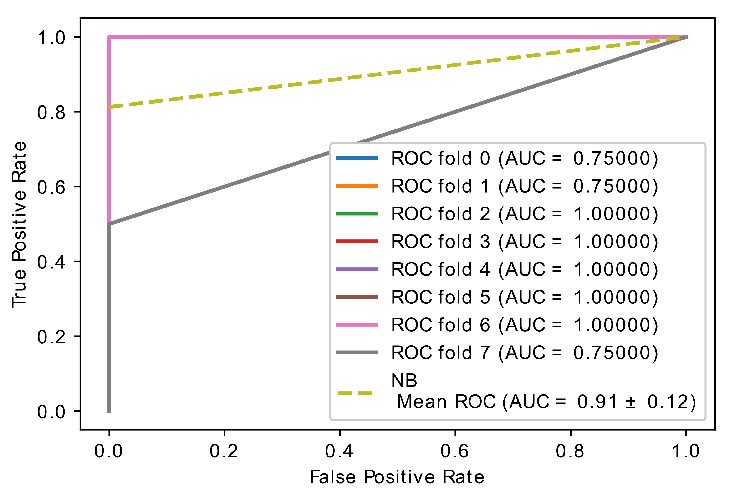
| Fold Number | Optimized CatBoost Classifier | |
|---|---|---|
| Train Accuracy | Test Accuracy | |
| 1 | 1.00 | 0.750 |
| 2 | 1.00 | 1.00 |
| 3 | 1.00 | 0.750 |
| 4 | 1.00 | 1.00 |
| 5 | 1.00 | 1.00 |
| 6 | 1.00 | 1.00 |
| 7 | 1.00 | 1.00 |
| 8 | 1.00 | 1.00 |
| Brain Cancer Dataset | CatBoost | Optimized CatBoost | ||||||
|---|---|---|---|---|---|---|---|---|
| Precision | Recall | f1-Score | Support | Precision | Recall | f1-Score | Support | |
| 0.0 | 0.85 | 0.79 | 0.81 | 14 | 0.92 | 0.79 | 0.85 | 14 |
| 1.0 | 0.80 | 0.86 | 0.83 | 14 | 0.81 | 0.93 | 0.87 | 14 |
| accuracy | 0.82 | 14 | 0.82 | 14 | ||||
| Macro avg | 0.82 | 0.82 | 0.82 | 28 | 0.82 | 0.82 | 0.82 | 28 |
| Weighted avg | 0.82 | 0.82 | 0.82 | 28 | 0.82 | 0.82 | 0.82 | 28 |
| Prob set | Gene ID | Gene Name | Diagnostic Marker | Prognostic Marker | Overexpression | Down Expression |
|---|---|---|---|---|---|---|
| 1860_at | 1860 | Tumor protein p53 binding protein 2(TP53BP2) | Unfavorable | + | ||
| 286_at | 286 | Histone cluster 2 H2A family member a4(HIST2H2AA4) | Yes | + | ||
| 31667_r_at | 31667_r | Nuclear receptor subfamily 2 group E member 3(NR2E3) | Yes | + | ||
| 33242_at | 33242 | TSR2, ribosome maturation factor(TSR2) | Yes | + | ||
| 34088_at | 34088 | Neurexophilin 4(NXPH4) | Unfavorable | + | ||
| 37055_at | 37055 | ETS variant 1(ETV1) | Unfavorable | + | ||
| 37701_at | 37701 | Regulator of G-protein signaling 2(RGS2) | Unfavorable | + | ||
| 40388_at | 40388 | DLG associated protein 1(DLGAP1) | Unfavorable | |||
| 41098_at | 41098 | Dishevelled associated activator of morphogenesis 2(DAAM2) | + | |||
| 1972_s_at | 1972_s | Microtubule associated protein 2(MAP2) | Unfavorable | + | ||
| 32647_at | 32647 | Vesicle transport through interaction with t-SNAREs 1B(VTI1B) | Yes | + | ||
| 36073_at | 36073 | Necdin, MAGE family member(NDN) | Unfavorable | + | ||
| 37360_at | 37360 | Lymphocyte antigen 6 complex, locus E(LY6E) | Yes | + | ||
| 38420_at | 38420 | Collagen type V alpha 2 chain(COL5A2) | Unfavorable | + | ||
| 39673_i_at | 39673_i | Extracellular matrix protein 2(ECM2) | Unfavorable | + | ||
| 41387_r_at | 41387_r | Lysine demethylase 6B(KDM6B) | Unfavorable | + | ||
| 41407_at | 41407 | MicroRNA 1236(MIR1236) | Unfavorable | + | ||
| 41725_at | 41725 | Casein kinase 1 gamma 2(CSNK1G2) | Unfavorable | + | ||
| 41732_at | 41732 | BolA family member 2(BOLA2) | Favorable | + | ||
| 103_at | 103 | Thrombospondin 4(THBS4) | Unfavorable | + | ||
| 1230_g_at | 1230_g | Myotubularin related protein 11(MTMR11) | Yes | + | ||
| 1396_at | 1396 | Insulin like growth factor binding protein 5(IGFBP5) | Unfavorable | + | ||
| 32988_at | 32988 | Chloride voltage-gated channel Ka(CLCNKA) | Unfavorable | + | ||
| 33854_at | 33854 | ATPase H+ transporting V1 subunit D(ATP6V1D) | Unfavorable | + | ||
| 37209_g_at | 37209_g | Phosphoserine phosphatase(PSPH) | Unfavorable | + | ||
| 35297_at | 35297 | NADH:ubiquinone oxidoreductase subunit AB1(NDUFAB1) | Unfavorable | + | ||
| 36155_at | 36155 | SPARC/osteonectin, cwcv and kazal-like domains proteoglycan 2(SPOCK2) | Favorable | + | ||
| 36534_at | 36534 | DIX domain containing 1(DIXDC1) | Unfavorable | + | ||
| 36617_at | 36617 | Inhibitor of DNA binding 1, HLH protein(ID1) | Unfavorable | + | ||
| 38440_s_at | 38440_s | Armadillo repeat containing, X-linked 6(ARMCX6) | Unfavorable | + | ||
| 39315_at | 39315 | Angiopoietin 1(ANGPT1) | Unfavorable | + | ||
| 39364_s_at | 39364_s | Protein phosphatase 1 regulatory subunit 3C(PPP1R3C) | Unfavorable | |||
| 39512_s_at | 39512_s | Inositol polyphosphate-4-phosphatase type I A(INPP4A) | + | |||
| 39850_at | 39850 | Ankyrin 2(ANK2) | Unfavorable | + | ||
| 755_at | 755 | Inositol 1,4,5-trisphosphate receptor type 1(ITPR1) | ||||
| 31386_at | 31386 | Immunoglobulin kappa variable 1/OR2-118 (IGKV1OR2-118) (pseudogene) | Unfavorable | + | ||
| 33580_r_at | 33580_r | Galanin receptor 3(GALR3) | + | |||
| 34193_at | 34193 | Cell adhesion molecule L1 like(CHL1) | Unfavorable | + | ||
| 35349_at | 35349 | COP9 signalosome subunit 3(COPS3) | Unfavorable | + | ||
| 35719_at | 35719 | PH domain and leucine rich repeat protein phosphatase 1(PHLPP1) | Unfavorable | + | ||
| 38967_at | 38967 | Chromosome 14 open reading frame 2(C14orf2) | Unfavorable | + | ||
| 39329_at | 39329 | Actinin alpha 1(ACTN1) | yes | Unfavorable | + | |
| 41530_at | 41530 | Acetyl-CoA acyltransferase 2(ACAA2) | Favorable | + | ||
| 38397_at | 38397 | DNA polymerase delta 4, accessory subunit(POLD4) | Unfavorable | |||
| 39008_at | 39008 | Ceruloplasmin(CP) | ||||
| 40767_at | 40767 | Tissue factor pathway inhibitor(TFPI) | Unfavorable | + | ||
| 41214_at | 41214 | Ribosomal protein S4, Y-linked 1(RPS4Y1) | Unfavorable | + | ||
| 31342_at | 31342 | Polypeptide N-acetylgalactosaminyltransferase 2(GALNT2) | Unfavorable | + | ||
| 32109_at | 32109 | FXYD domain-containing ion transport regulator 1(FXYD1) | yes | Unfavorable | + | |
| 32458_f_at | 32458_f | Proline rich protein BstNI subfamily 4(PRB4) | Unfavorable | + |
Publisher’s Note: MDPI stays neutral with regard to jurisdictional claims in published maps and institutional affiliations. |
© 2021 by the authors. Licensee MDPI, Basel, Switzerland. This article is an open access article distributed under the terms and conditions of the Creative Commons Attribution (CC BY) license (https://creativecommons.org/licenses/by/4.0/).
Share and Cite
Almars, A.M.; Alwateer, M.; Qaraad, M.; Amjad, S.; Fathi, H.; Kelany, A.K.; Hussein, N.K.; Elhosseini, M. Brain Cancer Prediction Based on Novel Interpretable Ensemble Gene Selection Algorithm and Classifier. Diagnostics 2021, 11, 1936. https://doi.org/10.3390/diagnostics11101936
Almars AM, Alwateer M, Qaraad M, Amjad S, Fathi H, Kelany AK, Hussein NK, Elhosseini M. Brain Cancer Prediction Based on Novel Interpretable Ensemble Gene Selection Algorithm and Classifier. Diagnostics. 2021; 11(10):1936. https://doi.org/10.3390/diagnostics11101936
Chicago/Turabian StyleAlmars, Abdulqader M., Majed Alwateer, Mohammed Qaraad, Souad Amjad, Hanaa Fathi, Ayda K. Kelany, Nazar K. Hussein, and Mostafa Elhosseini. 2021. "Brain Cancer Prediction Based on Novel Interpretable Ensemble Gene Selection Algorithm and Classifier" Diagnostics 11, no. 10: 1936. https://doi.org/10.3390/diagnostics11101936
APA StyleAlmars, A. M., Alwateer, M., Qaraad, M., Amjad, S., Fathi, H., Kelany, A. K., Hussein, N. K., & Elhosseini, M. (2021). Brain Cancer Prediction Based on Novel Interpretable Ensemble Gene Selection Algorithm and Classifier. Diagnostics, 11(10), 1936. https://doi.org/10.3390/diagnostics11101936