Survivability Analysis on a Cyber-Physical System

Abstract

A cyber-physical system (CPS) is composed of interdependent physical-resource and cyber-resource networks that are tightly coupled. The malfunction of nodes in a network may trigger failures to the other network and further cause cascading failures, which would potentially lead to the complete collapse of the entire system. The number and communication of operating nodes at stable state are closely related to the initial failure nodes and the topology of the network system. To address this issue, this paper studies the survivability of CPS in the presence of initial failure nodes, proposes (m, k)—survivability, which is defined as the probability that at least k nodes are still working in CPS after m nodes are attacked, and discusses the problem of cascading failure based on reliability (CFR). Further, we propose an algorithm to calculate (m, k)—survivability and find that the minimum survivability of system with regular allocation strategy decreases with k for a fixed m, and the proportion of initial failure node groups that cause the system to completely fragment increases with m. The simulation shows the properties and the result of CFR of the system with 12 nodes.

1. Introduction

A CPS consists of a physical network and a cyber network that are tightly coupled together and has been widely applied in many fields. Smart grid is a typical application of CPS. A power grid is covered on the computer network to realize the automation of the power grid and improve efficiency. The most striking feature of CPS is interdependency. Although interdependent networks make the system more intelligent and complex, Vespignani [1] showed that the system has greater vulnerability than a single network when facing attacks, failures, and natural disasters. A random removal of a small fraction of nodes from one network can cause an iterative cascade of failures in interdependent network and further lead to a disastrous impact on the overall cyber-physical system, such as 2003 blackout in the Northeastern United States and Southeastern Canada [2], and the electrical blackout that cause many losses in Italy on 28 September 2003 [3]. The cascading effect is one of the important characteristics of CPS. In the case of initial random node failures, cascading failures sometimes may not trigger complete collapse of CPS, resulting in several surviving nodes at steady state, such as micro grids. The network performance of surviving nodes is also an important issue to be addressed. In engineering, survivability is the quantified ability of a system, subsystem, equipment, process, or procedure to continue to function during and after a natural or man-made disturbance [4]. For CPS, the steady state is absolutely a subsystem of CPS and obtained after disturbance, i.e., random node failures. Survivability is consistent with the issue we address. Further, we focus on the communication ability of surviving nodes at steady state. Fortunately, reliability is an effective parameter to evaluate network performance and has been utilized in CPS [5]. In this article, we study the survivability of CPS based on reliability. For convenience, some definitions are listed as follows:

Definition 1 [6].

Suppose the edges of graph G never fail and the nodes fail independently with probability 1 − p, then the reliability of graph G is

$$R(G)={\displaystyle \sum _{r=1}^n{S}_r(G)P^r{(1-p)}^{n-r}}$$

(1)

where S_r(G) is the number of connected induced subgraphs of graph G that contain exactly r nodes.

All-terminal reliability with node failures describes the connectivity of all nodes in one network. Based on all-terminal reliability theory, Zhang et al. [5] gave k-reliability (denoted by R_k) which was defined as the probability that at least k surviving nodes of set V span an operating subgraph and defined cascading failures on reliability (CFR).

Definition 2 [5].

CFR, given constants k and R₀, if the number of surviving nodes at steady state in the case of random node failures is smaller than k or the k-reliability of steady state R_k < R₀, then random node failures have caused CFR of the CPS.

The definition is based on all-terminal reliability with node failures. For interdependence, cascading failures may occur after some nodes are attacked. All-terminal reliability with node failures can describe the connectivity of two networks. Therefore, it can represent the ability that the system can meet the required level of service when a certain number of nodes fail.

Based on these definitions, we propose (m, k)—survivability, which is defined as the probability that at least k nodes are still working in CPS after m nodes are attacked, and discuss the problem of cascading failure based on reliability. The proposed (m, k)—survivability reflects the connectivity of nodes in networks and illustrates the probability that the system meets the service requirements. Further, we propose an algorithm to calculate (m, k)—survivability and find that the minimum survivability of the system with a regular allocation strategy decreases with k for a fixed m, and the proportion of initial failure node groups that cause a system to fragment increases with m.

The rest of this paper is organized as follows. Section 2 shows background and related work. In Section 3, we introduce the definition of (m, k)—survivability and analyze cascading failures. Section 4 gives simulation and experiment to survivability of a CPS. The analysis and conclusion appear in Section 5 and Section 6, respectively.

2. Background and Related Work

The fragility of interdependent networks and designation of robust networks have been hot spots for CPS. Buldrev et al. [3] put forward a “one-to-one correspondence” model for interdependent networks and studied its robustness. They found that a random removal of a small fraction of nodes from one network can cause cascading failures and even complete fragmentation of interdependent networks. In order to estimate the robustness of the system, they calculated the size of functioning parts for each stage of cascading failures. Moreover, they presented a critical threshold p_c and showed that if the fraction of node failures 1 − p in one network satisfies p_c ≤ p, the two networks will completely fragment. Some literature [3] has received widespread attention and has aroused the interest of researchers in interdependent networks. Further research appears in different directions [7,8,9]. For instance, Buldyrev et al. [7] also considered the model in the case of “one-to-one correspondence,” but the difference from [3] is that mutually dependent nodes are assumed to have the same intraedges in their own networks. Shao et al. [9] considered multiple support-dependence relations between two coupled networks. They used a model where there existed some autonomously nodes in one network, meaning that these nodes can operate without supporting nodes from the other network. Furthermore, Yagan et al. [10] described the dynamic characteristics of cascading failures in the system where the topology of each individual network is unknown and showed that the regular allocation strategy has better robustness compared with all possible strategies. The above literature considers different CPS models and studies the robustness of CPS.

In engineering, survivability concepts appear in many other networks or research areas. For example, Neumann et al. [11] proposed the survivability definition of the network system for the first time. In a communication system, survivability is seen as the probability that its service is still available when the system is damaged or fails. Deutsh et al. [12] defined survivability in the context of software engineering, even if some parts of the system do not work and the basic services are reachable. Ellison et al. [13] discussed that survivability is the ability of the system to complete the task in time facing attacks, failures, and contingencies. Moitra et al. [14] argued that survivability is the ability of the system to resist the attack and to provide certain services after being attacked. In a wireless network, Panirahi [15] defined survivability as the ability of the system to complete its tasks in time for attacks, failures, and contingencies. Levitin et al. [16] argued that the survivability of information systems is the ability to maintain a working state when a fault event occurs. In the above article, the authors give different descriptive definitions of survivability. On the other hand, the study of survivability varies with researchers’ fields. Liang et al. [17] studied the survivability of time-varying networks and proposed a new survivability framework for time-varying networks. Wan et al. [18] researched the node survivability of a sensor network and considered how to schedule each sensor between active and sleep modes to maximize the network lifetime while meeting survival requirements. Petridou et al. [19] put forward a quantitative analysis for evaluating survivability of wireless sensor networks and defined four measures of network survivability: the frequency of failures, the data loss, the delay, and the compromised data under three different type of failures, namely, link, node, attack failures.

In the model of network reliability, K-terminal network reliability is the probability that G_k is connected, where G_k is a subgraph with specified k nodes [20]. Two nodes are connected to each other if there is a path between them in the network [21]. The following literature provides results ideal for calculating network reliability. Moskowitz [22] investigated a network model where nodes never fail, but each edge fails independently with probability. A factoring algorithm is put forward to calculate the reliability of network. On the basis of this result, Carlier et al. [23] applied a factoring algorithm and reductions to the network model in which vertices and edges may fail. As the calculation of network reliability is an NP-hard problem, the method of network reduction may reduce computation time. On the other hand, many studies have concentrated on approximating reliability. A discrete and dynamic model is defined to evaluate the reliability of telecommunication networks [24] and in this case, the set of terminals K of network is specified arbitrarily. Three methods were presented and they showed that failures have negative impact on service quality offered by network. Ayoub et al. [25] developed an algorithm that uses Monte–Carlo simulation and Breadth–First search to calculate the reliability of telecommunication networks. An exact reliability estimate was found by them in feasible and practical time after a sufficient number of simulations. The above researches on network reliability do not restrict the length of the path. Petingi et al. [26] proposed a polynomial-time algorithm for detecting and deleting irrelevant edges that make no difference to the source-to-terminal diameter constrained network reliability. They integrated this algorithm within an exact recursive factorization approach based upon Moskowitz’s edge decomposition, conducted on different real-world topologies and confirmed a substantial computational gain.

3. Survivability of Cyber-Physical Systems

A cyber-physical system is made up of two interacting networks, say, Networks A and B, both with N nodes, so the total number of nodes is n = 2N. We denote the node sets of A and B by 1, 2, …, N and N + 1, N + 2, …, n respectively. We call edges that connect different networks as interedges and those in the same network as intraedges. A node is functioning only if there is at least one interedge and one intraedge. We are concerned with whetheer the system exists functioning giant component [10] or completely separated when cascading failures occur.

Definition 3.

If m nodes are attacked, the probability that at least k nodes still operate is called (m, k)—survivability, denoted by S (m, k).

Discussion: Definition 3 does not indicate where the m nodes are located and thus imply the best-case and worst-case survivability. The parameter m is the number of failed nodes in the system, and the parameter k indexes the communication quality of surviving nodes with node failures. Actually, S (m, k) with all possible m and k is a matrix.

For any 1 ≤ k ≤ n, 1 ≤ m ≤ n,

$$S(m,k):=\left[\begin{array}{cccccc}{S}_{11}& S_{12}& S_{13}& \dots & S_{1,n-1}& S_{1n}\\ S_{21}& S_{22}& S_{23}& \dots & S_{2,n-1}& S_{2n}\\ S_{31}& S_{32}& S_{33}& \dots & S_{3,n-1}& S_{3n}\\ \dots & \dots & \dots & \dots & \dots & \dots \\ S_{n-1,1}& S_{n-1,2}& S_{n-1,3}& \dots & S_{n-1,n-1}& S_{n-1,n}\\ S_{n1}& S_{n2}& S_{n3}& \dots & S_{n,n-1}& S_{nn}\end{array}\right]$$

where S_ij denotes the probability that there has at least j nodes are still working after i nodes are attacked. Obviously, the locations of node failures may cause different steady state. Thus, S_ij is a vector where the elements denote the survivability after i nodes in different positions are invalidated. That is, S_ij = {S_x (i, j) | 1 ≤ x ≤ C_nⁱ}. The survivability S_x (i, j) is stated mathematically as follows:

$$S_x(i,j)={\displaystyle \sum _{r=j}^{\left|V_x\right|}{S}_r(G)P^r{(1-p)}^{\left|V_x\right|-r}}$$

(2)

where 1 ≤ x ≤ C_nⁱ, S_x (i, j) is the survivability of system after the xth combination of i nodes are invalidated. |V_x| is the number of nodes in the steady state.

We propose an Algorithm 1 based on network reliability method in the presence of initial node failures.

Algorithm 1: (m, k)—survivability in G = (V, E)

Input: A connected graph G = (V, E) with the node set V, edge set E, and node probability p require the number of normal work k and failure nodes m.

Output: (m, k)—survivability S (m, k) of G = (V, E).

Step 0. Let M = ∅.

Step 1. Choose all the endpoint groups with m numbers, and store them into the collection M.

Step 2. For each group v $\in$ M, obtain the adjacency matrix A of steady state.

Step 3. Let s = 0, r = k, S = ∅, Sr = 0.

Step 4. calculate the node number of steady state n1 for each terminal nodes groups, find all the connected endpoint sets of r, and stored in the collection S.

Step 5. Sr = |S|.

Step 6. R = R + Sr * pr * (1 − p )n1-r.

Step 7. r = r + 1, S = ∅, go to Step 4.

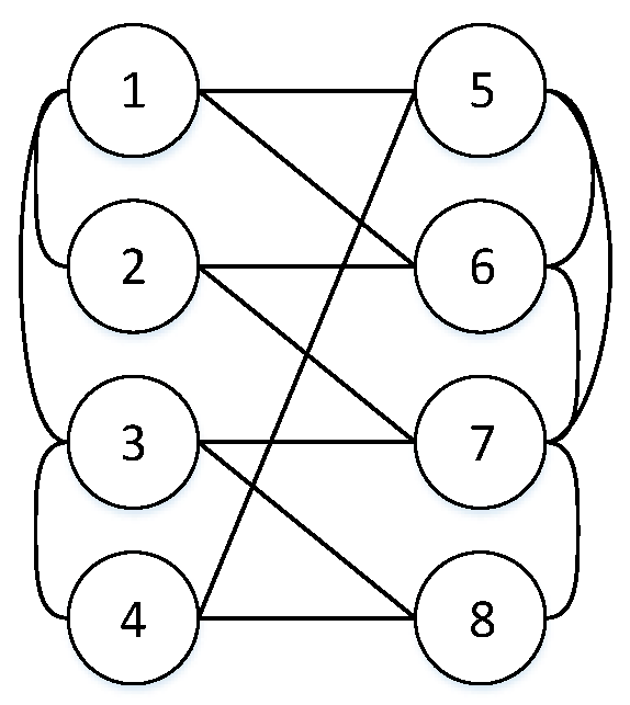
The complexity of computation: First step, choosing all groups is based on permutation and combination theory and belongs to the NP-hard problem. That is, for a given m, we need to choose $\left(\begin{array}{c}n\\ m\end{array}\right)=\frac{n!}{(n-m)!m!}$ groups of nodes. For example, in Figure 1, i = 1 and j = 2.

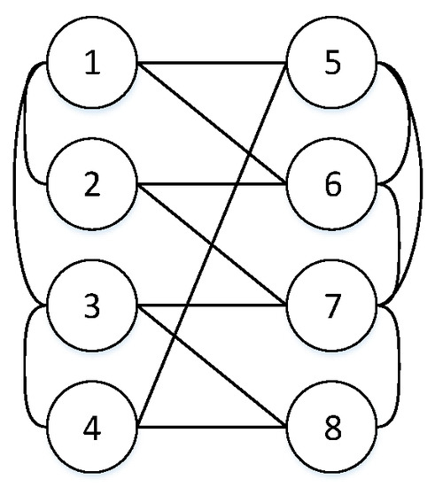
Figure 1. A CPS with 8 nodes.

Then, S (1,2) = {S_x (1,2) | 1 ≤ x≤ 8}. According to Equation (2), we can obtain

S (1,2) = {0.9898, 0.9950, 0.9979, 0.9973, 0.9877, 0.9877, 0.9869, 0.9885}.

Especially, if the indices i and j satisfy i + j > n, then the corresponding elements of the matrix are zero, and the actual situation means no surviving nodes. Therefore, the matrix can be written as

$$S(m,k)=\left[\begin{array}{cccccc}{S}_{11}& S_{12}& S_{13}& \dots & S_{1,n-1}& 0\\ S_{21}& S_{22}& S_{23}& \dots & 0& 0\\ S_{31}& S_{32}& S_{33}& \dots & 0& 0\\ \dots & \dots & \dots & \dots & \dots & \dots \\ S_{n-1,1}& 0& 0& \dots & 0& 0\\ 0& 0& 0& \dots & 0& 0\end{array}\right].$$

In order to explore the survivability of CPS, we analyze the nonzero elements in the matrix.

For any i and j, S_ij is a vector of length C_nⁱ. We use $\stackrel{-}{S}$_ij to denote the average of S_ij. The corresponding matrix is

$$\stackrel{-}{S_{mk}}=\left[\begin{array}{cccccc}{\stackrel{-}{S}}_{11}& {\stackrel{-}{S}}_{12}& {\stackrel{-}{S}}_{13}& \dots & {\stackrel{-}{S}}_{1,n-1}& 0\\ {\stackrel{-}{S}}_{21}& {\stackrel{-}{S}}_{22}& {\stackrel{-}{S}}_{23}& \dots & 0& 0\\ {\stackrel{-}{S}}_{31}& {\stackrel{-}{S}}_{32}& {\stackrel{-}{S}}_{33}& \dots & 0& 0\\ \dots & \dots & \dots & \dots & \dots & \dots \\ {\stackrel{-}{S}}_{n-1,1}& 0& 0& \dots & 0& 0\\ 0& 0& 0& \dots & 0& 0\end{array}\right]$$

An average is a measure of the trend in a set of data sets. Through the above matrix, we can get the average survival level of the system for different m- and k-values. If the average value is large, it shows that the system has strong survivability when m nodes are attacked. Otherwise, it has weak survivability.

For the interdependent network, whether the system is still to provide a certain service after some nodes are attacked is concerned problem. Thus, we give the following definition.

Definition 4.

Given a constant R₀, S (m, k) is associated with a pair of (m, k), 1 ≤ i ≤ C_n^m,

(1)

If max S_i (m, k) < R₀, we say the cyber-physical system is not (m, k)—survivable and has occurred cascading failures, denoted by (m, k)—CF.

(2)

If min S_i (m, k) > R₀, the cyber-physical system is robust (m, k)—survivable, denoted by (m, k)—RS.

(3)

If min S_i (m, k) < R₀ < max S_i (m, k), let Ω₁(m, k) denotes the set of the node groups that let S_i (m, k) < R₀ hold. The node groups in Ω₂(m, k) satisfy S_i (m, k) > R₀. | Ω₁(m, k) | and | Ω₂(m, k) | denote the number of node groups, respectively. If | Ω₁(m, k) | ≥ | Ω₂(m, k) |, we say the system is (m, k)—frail, denoted by (m, k)—FR. If | Ω₁(m, k) | < | Ω₂(m, k) |, the system is weak (m, k)—survivable, denoted by (m, k)—WS.

We consider a critical value to determine whether node-attacks cause cascading failures. Different from [5], we require the maximum, minimum survivability, and the number of node groups that are less or more than R₀. The situations where k = 0 or R₀ = 1 are specifically discussed in [2], and situation k = |V| indicates the all-terminal reliability of the system. |V| denotes the number of nodes at steady state. The value of R₀ is related to m and k.

For example, in Figure 1, R₀ = 0.98, and min S (1,2) > R₀, then the system is (1,2)—RS, max S (1,5) = 0.9743 < R₀ = 0.98, so the system is (1,5)—CF. | Ω₁(2,3) | = 9 < | Ω₂(2,3) | = 21, so the system is (2,3)—WS. Given an R₀ = 0.95, | Ω₁(2,4) | = 18 > | Ω₂(2,4) | = 10, so the system is (2,4)—FR.

The regular allocation strategy is to allocate the same number of bidirectional inter-links to each node of the system. We study the systems with regular allocation strategy and have the following results.

Proposition 1.

For a fixed m, the survivability of CPS decreases monotonously with k for the same locations.

Proof. 

Assume that the xth combination of m nodes are attacked, the number of nodes in steady state is |V_x|. For any 1 ≤ k ≤ |V_x|, 1 ≤ x ≤ C_n^m.

$$\begin{array}{l}{S}_x(m,k)={\displaystyle \sum _{r=k}^{\left|V_x\right|}{S}_r(G)p^r{(1-p)}^{\left|V_x\right|-r}}={\displaystyle \sum _{r=k+1}^{\left|V_x\right|}{S}_r(G)p^r{(1-p)}^{\left|V_x\right|-r}}\\ +S_k(G)p^k{(1-p)}^{\left|V_x\right|-k}\ge S_x(m,k+1).\end{array}$$

For example, in Figure 1a, m = 1 and 1 ≤ k ≤ 7, so

S₄(1, k) = {0.9973,0.9973,0.9972,0.9953,0.9743,0.8503,0.4783}.

Therefore, the survivability of CPS decreases monotonously with k at the same position.

Proposition 2.

The survivability of a graph G = (V, E) is not less than that of its subgraphs if same locations are attacked.

Proof. 

Assume that G* = (V*, E*) is a subgraph of G = (V, E), where V* $\subseteq$ V, E* $\subseteq$ E. |V^*_x| and |V_x| denote the number of nodes in steady state after the xth combination of m nodes are attacked and |V^*_x|<|V_x|.

First, if |V*| ≤ m, then the inequality is satisfied.

If |V*| > m and k < |V^*_x|, E_k denotes the events that k nodes work after m nodes are attacked. Hence, the survivability of G can be calculated by

S_x(m, k) = P(E_k ∪ E_k+1 ∪ ⋯ ∪ E_|Vx|).

The survivability of subgraph G* can be calculated by

S*_x(m, k) = P(E*_k ∪ E*_k+1 ∪ ⋯ ∪ E*_|V*x|)

where G* = (V*, E*) is a subgraph of G = (V, E), hence {E_k , …, E_|Vx|} $\supseteq$ {E*_k , …, E*_|V*x|}.

Let {E_k , …, E_|Vx|} = {E_k , …, E_|V*x|, E_|V*x|+1,…, E_|Vx|}, where E_k $\supseteq$ E*_k,…, E_|V*x| $\supseteq$ E*_|V*x|.

According to the probability theory, we obtain

S_i(m, k) = P(E_k ∪ E_k+1 ∪ ⋯ ∪ E_|Vx|) = P(E_k ∪ E_k+1 ∪ ⋯ ∪ E_|V*x| ∪ E_|V*x|+1 ∪ ⋯ E_|Vx|)

≥ P(E*_k∪E*_k+1 ∪ ⋯ ∪E*_|V*x|)

= S*_x(m, k).

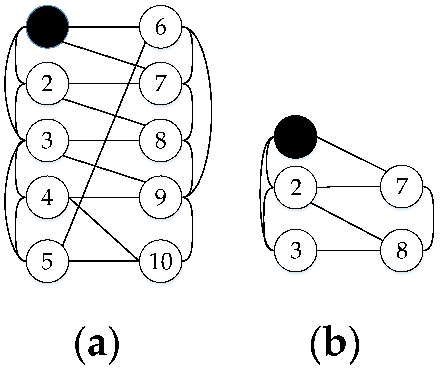
For example, Figure 2b is subgraph of (a), when same nodes are attacked, steady state of (b) is subgraph of (a). Accordingly, the survivability of (a) is better than (b).

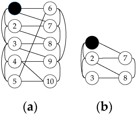
Figure 2. (a) is a CPS with 10 nodes and (b) is its subgraph.

From Propositions 1 and 2, the survivability of the system is closely related to m and k. Therefore, it is meaningful to evaluate CPS by checking m and k of the survivability.

Proposition 3.

For a fixed m, the number of initial failed node groups that provide the system with minimal survivability increases monotonically as k increases.

Proof.

According to Proposition 1, the survivability of CPS decreases monotonously with k at the same position. n_k and n_k+1 denote the number of initial failure node groups that provide the system with minimal survivability respectively. N_k and N_k+1 denote the set of initial failure node groups that provide the system with minimal survivability respectively. Then N_k ⊆ N_k+1, so n_k ≤ n_k+1.

We also study the robustness of system with regular allocation strategy. Let n_s denote the number of remain nodes of system at steady state. Then, for a fixed m, n_s is a vector of length C_n^m. We use average number of remain nodes of n_s (denoted by ANRN) to describe the robustness of entire system macroscopically. And we have follow result on robustness.

Proposition 4.

The proportion of node groups that cause the system to completely fragment increases with m.

Proof. 

V_m denote the set of node groups that cause the system to completely separate for a fixed m. Therefore, V_m ⊆ V_m+1. According to | V_m+1|≥C_n-m¹ | V_m | and C_n^m+1 = $\frac{m+1}{n-m}$ C_n^m, we can obtain $\frac{\left|V_m\right|}{{{\displaystyle C}}_n^m}\le \frac{\left|V_{m+1}\right|}{{{\displaystyle C}}_n^{m+1}}$.

4. Simulation and Examples

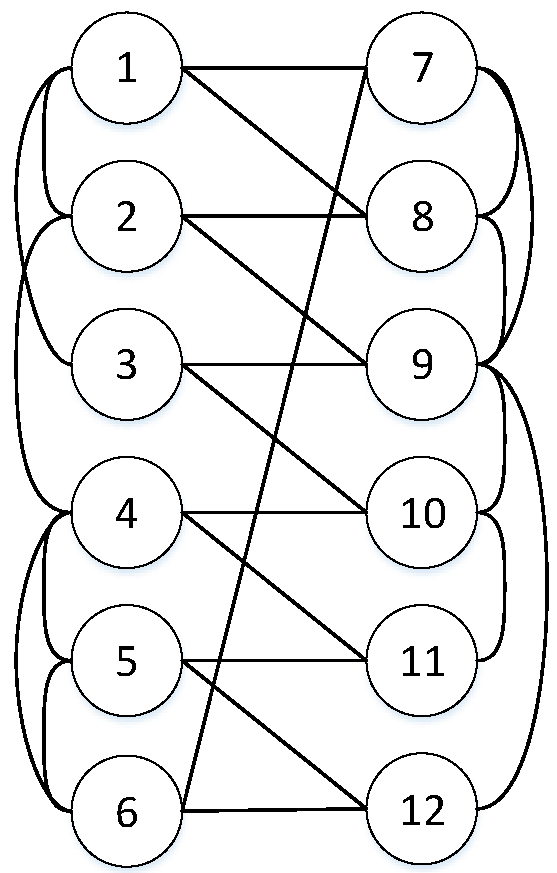
In this part, we choose a CPS with a regular allocation strategy to simulate and experiment. Each network has six nodes, and each node has the same interedges that are assumed to be bidirectional. Let the reliability of each node be p = 0.9. Network topology is shown in Figure 3.

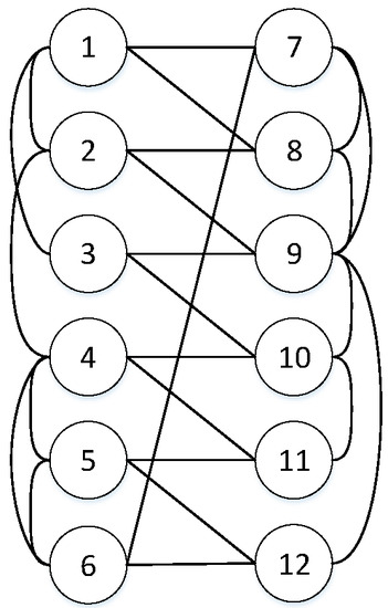
Figure 3. Instance with n = 12 nodes for survivability where Networks A and B have both six nodes.

According to the definition, we obtain the following (m, k)—survivability matrix:

$$S(m,k):=\left[\begin{array}{cccccc}{S}_{11}& S_{12}& S_{13}& \dots & S_{1,11}& S_{1,12}\\ S_{21}& S_{22}& S_{23}& \dots & S_{2,11}& S_{2,12}\\ S_{31}& S_{32}& S_{33}& \dots & S_{3,11}& S_{3,12}\\ \dots & \dots & \dots & \dots & \dots & \dots \\ S_{11,1}& S_{11,2}& S_{11,3}& \dots & S_{11,11}& S_{11,12}\\ S_{12,1}& S_{12,2}& S_{12,3}& \dots & S_{11,12}& S_{12,12}\end{array}\right]$$

Then, in order to analyze the survivability of this system, we need to calculate each element. First, according to the above results, if i + j > 12, S_ij = 0. Therefore, we get the following simplified matrix. The corresponding average matrix is

$$S(m,k)=:\left[\begin{array}{cccccc}{S}_{11}& S_{12}& S_{13}& \dots & S_{1,11}& 0\\ S_{21}& S_{22}& S_{23}& \dots & 0& 0\\ S_{31}& S_{32}& S_{33}& \dots & 0& 0\\ \dots & \dots & \dots & \dots & \dots & \dots \\ S_{11,1}& 0& 0& \dots & 0& 0\\ 0& 0& 0& \dots & 0& 0\end{array}\right]\stackrel{-}{S_{mk}}=:\left[\begin{array}{cccccc}{\stackrel{-}{S}}_{11}& {\stackrel{-}{S}}_{12}& {\stackrel{-}{S}}_{13}& \dots & {\stackrel{-}{S}}_{1,11}& 0\\ {\stackrel{-}{S}}_{21}& {\stackrel{-}{S}}_{22}& {\stackrel{-}{S}}_{23}& \dots & 0& 0\\ {\stackrel{-}{S}}_{31}& {\stackrel{-}{S}}_{32}& {\stackrel{-}{S}}_{33}& \dots & 0& 0\\ \dots & \dots & \dots & \dots & \dots & \dots \\ {\stackrel{-}{S}}_{11,1}& 0& 0& \dots & 0& 0\\ 0& 0& 0& \dots & 0& 0\end{array}\right]$$

Next, we analyze the remain elements of the matrix. The mean and minimum value of survivability for different m- and k-values are given, and we also obtain the number of initial failure node groups that provide the system with minimal survivability. The results are as follows (Table 1):

Table 1. The mean and minimum value of survivability for different m- and k-values and the number of initial failure node groups that provide the system with minimal survivability. (The first parameter indicates the mean survivability. The second parameter indicates minimum survivability. The third parameter indicates the number of node groups).

	k	2	4	6	8	9	10	11
m
1		0.9836	0.9836	0.9831	0.9492	0.8365	0.5811	0.2354
		0.9575	0.9574	0.9534	0.7748	0.3874	0	0
		1	1	1	1	1	1	1
2		0.9389	0.9081	0.8204	0.6462	0.4226	0.1585
		0	0	0	0	0	0
		2	2	8	13	21	36
3		0.7972	0.7336	0.5039	0.2483	0.0863
		0	0	0	0	0
		38	38	91	132	171
4		0.5712	0.4953	0.2062	0.0383
		0	0	0	0
		204	204	361	451
5		0.3429	0.2781	0.0497
		0	0	0
		515	515	731
6		0.1693	0.1282	0.0063
		0	0	0
		765	765	913
7		0.0634	0.0449
		0	0
		741	741
8		0.0139	0.0093
		0	0
		488	488
9		0
		0
		220
10		0
		0
		66

In Table 2, we give a constant R₀ for different m- and k-values to estimate the survivability of the system.

Table 2. Cascading failure evaluation for Figure 3.

m	k	R0	max	min	|Ω1|	|Ω2|	Survivability
1	2	0.99	0.9935	0.9575	7	5	(1,2)-FR
1	5	0.95	0.9935	0.9571	0	12	(1,5)-RS
2	4	0.98	0.9916	0	49	17	(2,4)-FR
2	6	0.90	0.9908	0	15	51	(2,6)-WS
3	5	0.90	0.9874	0	124	96	(3,5)-FR
4	6	0.7	0.9566	0	405	90	(4,6)-FR
5	4	0.8	0.9848	0	654	138	(5,4)-FR
6	4	0.7	0.9776	0	872	52	(6,4)-FR
7	3	0.7	0.9914	0	741	51	(7,3)-FR
8	4	0.5	0.6561	0	488	7	(8,4)-FR
9	1	0	0	0	220	0	(9,1)-CF
10	1	0	0	0	66	0	(10,1)-CF
11	1	0	0	0	12	0	(11,1)-CF

In Table 3, we give the number and proportion of node groups that cause the system to fragment and average remain nodes for any m. When m > 9, the system always collapses. Therefore, we just analyze m < 9.

Table 3. The number and proportion of node groups that cause the system to completely fragment and ANRN with 12 nodes.

m	Proportion	Number	ANRN	m	Proportion	Number	ANRN
1	0	0	10.6667	5	0.6505	515	1.6793
2	0.0303	2	8.4091	6	0.8279	765	0.7565
3	0.1727	38	5.6727	7	0.9356	741	0.2677
4	0.4121	204	3.2788	8	0.9859	488	0.0566

5. Discussion

The average survivability can represent a variation trend of survivability of a system for different m- and k-values macroscopically. From Table 1, the mean survivability of the system decreases with the parameters k and m. When both m and k are small, the system has a strong survivability; i.e., when m nodes are attacked, the system has a great probability that k nodes are still working. It represents that the ability which the system satisfies the specified level of service is great. Otherwise, the system has weak survivability; i.e., the system has a small probability that k nodes are still working and the ability which the system satisfies the specified level of service is not good. Moreover, when m > 9, the mean survivability is always equal zero. It shows that the system always collapses as m > 9. For other values, some node groups cause the system to collapse, and the system has the best survivability after it is attacked by other node groups. The second parameter indicates that the minimum survivability decreases with k for a fixed m. That is, the minimum probability that k nodes are still functioning decreases with k when m nodes are attacked. We also find the number of initial failure node groups that provide the system with minimal survivability increase with k for a fixed m. Let $p=n_k/C_n^m$ if an intelligent adversary chooses some nodes to attack, we can know what the probability of getting the worst impact is. From Table 2, the survivability of the system changes as R₀, m and k vary. R₀ is a critical threshold to determine the impact that random attacks cause. Moreover, the system experiences cascading failure as m > 9 and R₀ = 0. From Table 3, we can see that the average of the remain node decreases with m. The nodes groups that cause the system to fragment increases with m. The other two sets of data illustrate this point. The more nodes of failure there are, the less ability to reach the specified service the system will have.

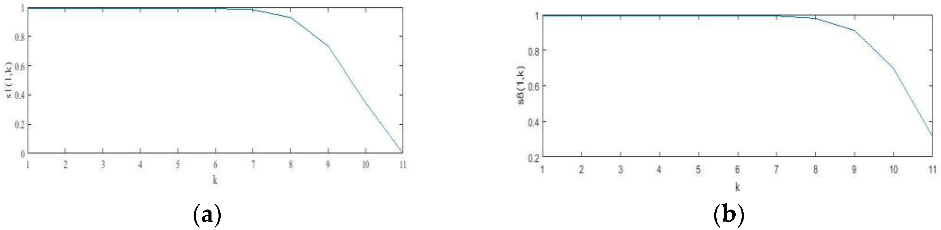
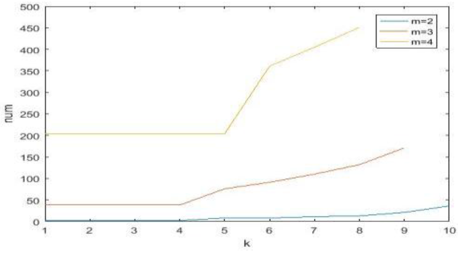
For a clearer explanation of Propositions 1 and 3, see Figure 4, wherein the image of S₁(1, k), S₈(1, k) changes with k. The image of num changes with k for a fixed m in Figure 5.

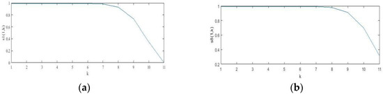
Figure 4. The image of (a) S₁(1, k); (b) S₈(1, k) with different k-values.

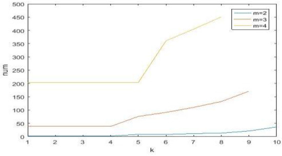
Figure 5. The image of num with different k-values.

6. Conclusions

We investigate the survivability problem of a cyber-physical system and define survivability of the cyber-physical system, namely (m, k)—survivability. By analyzing (m, k)—survivability, we find that the survivability of a system with a regular allocation strategy is not less than that of its subsystem for given node failures and for a fixed m, the number of initial failed node groups that provide the system with minimal survivability increases monotonically as k increases. We also find that the proportion of node groups that cause the system to completely fragment increases with m. Therefore, the survivability of a system is closely related to m and k. Our results are beneficial for network design. For example, the evaluation of survivability can be used to predict whether a designed network can meet given requirements and a certain level of communication quality. As for future work, we will research the survivability of a system with a random allocation strategy and a unidirectional interedge allocation strategy. Furthermore, we will investigate the relationship between threshold R₀ and the network.

References

- Vespignani, A. Complex networks: The fragility of interdependency. Nature 2010, 464, 984–985. [Google Scholar] [CrossRef] [PubMed]
- Parshani, R.; Buldyrev, S.V.; Havlin, S. Interdependent networks: Reducing the coupling strength leads to a change from a first to second order percolation transition. Phys. Rev. Lett. 2010, 105, 048701. [Google Scholar] [CrossRef] [PubMed]
- Buldyrev, S.V.; Parshani, R.; Paul, G.; Stanley, H.E.; Havlin, S. Catastrophic cascade of failures in interdependent networks. Nature 2010, 464, 1025–1028. [Google Scholar] [CrossRef] [PubMed]
- Wikipedia. Available online: https://en.wikipedia.org/wiki/Survivability (accessed on 31 July 2017).
- Zhang, Z.Y.; An, W.; Shao, F.M. Cascading Failures on Reliability in Cyber-Physical System. IEEE Trans. Reliab. 2016, 65, 1745–1754. [Google Scholar] [CrossRef]
- Wang, Y.-Q. Nearly regular complete bipartite graphs are locally most reliable. Appl. Math. J. Chin. Univ. 2003, 18, 365–370. [Google Scholar]
- Buldyrev, S.V.; Shere, N.W.; Cwilich, G.A. Interdependent Networks with Identical Degrees of Mutually Dependent Nodes. Phys. Rev. E 2011, 83, 016112. [Google Scholar] [CrossRef] [PubMed]
- Cho, W.; Goh, K.I.; Kim, I.M. Correlated Couplings and Robustness of Coupled Networks. arXiv, 2010; arXiv:arXiv:1010.4971v1. [Google Scholar]
- Shao, J.; Buldyrev, S.V.; Havlin, S.; Stanley, H.E. Cascade of Failures in Coupled Network Systems with Multiple Support Dependent Relations. Phys. Rev. E. 2011, 83, 036116. [Google Scholar] [CrossRef] [PubMed]
- Yagan, O.; Qian, D.J.; Zhang, J.; Cochran, D. Optimal allocation of inter-connecting links in cyber-physical systems: Interdependence, cascading failures and robustness. IEEE Trans. Parallel Distrib. Syst. 2012, 23, 1708–1720. [Google Scholar] [CrossRef]
- Neumann, P.G.; Barnes, A.H. Survivable Computer-Communication Systems: The Problem and Working Group Recommendations; Technical Report VAL-CE-TR-92-22; US Army Research Laboratory: Washington, DC, USA, 1993. [Google Scholar]
- Deutsch, M.S.; Willis, R.R. Software Quality Engineering: A Total Technical and Management Approach; Prentice-Hall: Englewood Cillfs, NJ, USA, 1988. [Google Scholar]
- Ellison, R.J.; Fisher, D.A.; Linger, C. Survivability: Protecting Your Critical Systems. IEEE Int. Comput. 1999, 3, 55–63. [Google Scholar] [CrossRef]
- Moitra, S.D.; Konda, S.L.A. Simulation Model for Managing Survivability of Network Information Systems; Technical Report CMU/SEI-2000-TR-020; Software Engineering Institute–Carnegie Mellon University: Pittsburgh, PA, USA, 2000. [Google Scholar]
- Panirahi, D. Survivable network design problems in wireless networks. In Proceedings of the Twenty-Second Annual ACM-SIAM Symposium on Discrete Algorithms, San Francisco, CA, USA, 23–25 January 2011; pp. 1014–1027. [Google Scholar]
- Levitin, G.; Hausken, K.; Taboada, H.A.; Coit, D.W. Survivability vs. security in information systems. Reliab. Eng. Syst. Saf. 2012, 100, 19–27. [Google Scholar] [CrossRef]
- Liang, Q.; Modiano, E. Survivability in Time-varying Networks. IEEE Trans. Mob. Comput. 2016. [Google Scholar] [CrossRef]
- Wan, X.; Wu, J.; Shen, X. Maximal Lifetime Scheduling for Roadside Sensor Networks With Survivability k. IEEE Trans. Veh. Technol. 2015, 64, 5300–5313. [Google Scholar] [CrossRef]
- Petridou, S.; Basagiannis, S.; Roumeliotis, M. Survivability Analysis Using Probabilistic Model Checking: A Study on Wireless Sensor Networks. IEEE Syst. J. 2013, 7, 4–12. [Google Scholar] [CrossRef]
- Wood, R.K. Factoring algorithms for computing K-terminal network reliability. IEEE Trans. Reliab. 1986, R-35, 269–278. [Google Scholar] [CrossRef]
- Bollob´as, B. Random Graphs. Cambridge Studies in Advanced Math; Cambridge University Press: Cambridge, UK, 2001. [Google Scholar]
- Moskowitz, F. The analysis of redundancy networks. AIEE Trans. Commun. Electron. 1958, 39, 627–632. [Google Scholar] [CrossRef]
- Carlier, J.; Theologou, O. Factoring & reductions for networks with imperfect vertices. IEEE Trans. Reliab. 1991, 40, 210–217. [Google Scholar]
- Adjabi, S.; Bouchama, K. K-terminal reliability evaluation of a telecommunications network represented by a discret and a dynamic model. Int. J. Oper. Res. 2011, 8, 34–43. [Google Scholar]
- Ayoub, J.N.; Saafm, W.H.; Kahhaleh, B.Z. K-terminal reliability of communication network. In Proceedings of the 7th IEEE International Conference on Electronics, Circuits and Systems, Jounieh, Lebanon, 17–20 December 2000; Volume 1, pp. 374–377. [Google Scholar]
- Cancela, H.; Petingi, L.A. Polynomial-time topological reductions that preserve the diameter constrained reliability of a communication network. IEEE Trans. Reliab. 2011, 60, 845–851. [Google Scholar] [CrossRef]
© 2017 by the authors. Licensee MDPI, Basel, Switzerland. This article is an open access article distributed under the terms and conditions of the Creative Commons Attribution (CC BY) license (http://creativecommons.org/licenses/by/4.0/).