Sensorless Sector Determination of Brushless DC Motors Using Maximum Likelihood Estimation

Abstract

Brushless DC motors are widely used for their high power density and efficiency. However, sensorless control remains challenging due to the difficulty of accurate rotor position detection, especially at low speeds. This paper proposes a novel sensorless trapezoidal control method based on Maximum Likelihood Estimation (MLE) for rotor sector detection. Unlike conventional back-EMF zero-crossing techniques, the proposed method uses a statistical algorithm to generate a probability map from prior motor state data, enabling accurate rotor position estimation without sensors. The MLE method operates with a typical computation time of 50–100 $\mathrm{\mu }$s, offering a balanced tradeoff between speed and accuracy. It is significantly faster than Kalman filter-based approaches (200–1000 $\mathrm{\mu }$s) and comparable to observer-based methods (20–80 $\mathrm{\mu }$s), while being more robust than zero-crossing techniques (<5 $\mathrm{\mu }$s). This makes it a practical and cost-effective solution for applications demanding high efficiency and reliability, such as electric mobility systems.

1. Introduction

Brushless DC motors are increasingly extensive across the computing, automotive and consumer appliance, and industrial automation sectors thanks to their efficiency, compact size, torque density, wide speed controllability, and minimal maintenance requirements. Placing permanent magnets on the rotor side provides brushless DC machines with significantly higher power density and efficiency compared to both brushed DC and induction motors [1,2].

Their ability to achieve accurate commutation timing is crucial to preventing locked-rotor conditions and enabling high-performance operation. Traditional solutions rely on mechanical shaft encoders or Hall-effect sensors to sensitively determine rotor position [3,4]; however, these sensors increase system cost, reduce reliability, and complicate maintenance. Consequently, sensorless control methods which eliminate physical sensors while maintaining performance have become a major research focus.

Among sensorless approaches, the Zero-Crossing Point Detection (ZCPD) method remains the simplest and most widely used method in industrial applications. It detects back-EMF (Back Electromotive Force) zero crossings via voltage comparators and filtering circuits [5,6,7,8,9]. While the simplicity of ZCPD is suitable for low-cost systems, it has drawbacks due to its sensitivity to Pulse Width Modulation (PWM) interference and Electromagnetic Interference (EMI). Its analog filtering also causes delay and distortion, especially under high-speed changes.

Advanced alternatives of this method have been proposed in recent years, one of which is back-EMF integration. This method improves sensitivity, but can accumulate error over time [10]. Other methods include flux-linkage-based techniques such as those employing motor magnetic models; these offer more precise estimation but are highly dependent on accurate modeling, which becomes problematic under parameter variations such as temperature or saturation [11]. In addition to those strategies, methods such as freewheeling conduction detection increase hardware complexity without universally improving robustness [12].

Recently, machine learning-based and data-driven methods have gained popularity for sensorless brushless DC motor control. Wang et al. applied back-EMF feature classification using support vector machines [11], while Chen et al. introduced deep learning-based torque and position estimation frameworks [13]. These techniques demonstrate significant changes in the field; however, the extensive training datasets and heavy computational complexity problems of these methods challenges real-time embedded deployment.

To address the tradeoffs between robustness, accuracy, and implementation simplicity, a novel sensorless commutation strategy based on Maximum Likelihood Estimation (MLE) is proposed in this paper. In the proposed method, commutation sector detection is formulated as a probabilistic classification task from back-EMF signals for each predefined sector. These are modeled using probability density functions, and the most probable sector is estimated statistically. The proposed strategy enhances robustness over a wide speed range without the need for complex modeling or additional hardware. Moreover, because the likelihood computation involves a fixed number of multiplications and additions, the method has high computational efficiency, making it particularly suitable for embedded implementation on microcontrollers such as those in the Texas Instruments C2000 family (Dallas, TX, USA).

It is worth noting that recent studies such as those by Soni and Tripathi [14] have investigated sensorless brushless DC control at ultra-high speeds exceeding 10,000 rpm. These works demonstrate the relevance of such regimes for specialized high-speed drive systems. However, in the present study the focus is placed on Light Electric Vehicle (LEV) applications, where such extreme rotational speeds are not typically encountered due to drivetrain limitations, safety standards, and motor design constraints. Therefore, the operating speed envelope considered in this paper is intentionally bounded within the practical range of LEV use cases. Despite this, the proposed MLE-based algorithm is not inherently limited to moderate speeds, and its extension to ultra-high-speed regimes remains a promising direction for future work.

2. Mathematical Model of Brushless DC Motor

Brushless DC motors are often used in the powertrains of light electric vehicles due to their high power density and efficiency. As in all electromechanical energy conversion systems, brushless DC motors are modeled with equations for both the electrical and mechanical sides. Due to the very low electrical conductivity of permanent magnets, the induced voltages and losses on the rotor can be neglected in the brushless DC motor model [15]. The electrical-side equations obtained for each phase winding are provided in (1), where $V_a$, $V_b$, and $V_c$ have applied stator voltage, R is stator resistance, L is stator inductance, and $e_a$, $e_b$, and $e_c$ are the back-EMF for each phase [16].

$$V_{abc}=R{i}_{abc}+L{\displaystyle \frac{d{i}_{abc}}{dt}}+e_{abc}$$

(1)

The term back-EMF is a type of reverse voltage induced on the stator side by the movement of permanent magnets in the rotor, and its behavior should be modeled as a function of rotor position [17]. The back-EMF equations are given in (2)–(4) for each phase. where $K_e$ is the back-EMF constant, ${\theta }_e$ is rotor angle, ${\omega }_m$ is rotor angular speed, $f\left({\theta }_e\right)$ is the trapezoidal back-EMF generator function.

$$e_a=K_{e}f\left({\theta }_e\right){\omega }_m$$

(2)

$$e_b=K_{e}f({\theta }_e-{\displaystyle \frac{2\pi }{3}}){\omega }_m$$

(3)

$$e_c=K_{e}f({\theta }_e+{\displaystyle \frac{2\pi }{3}}){\omega }_m$$

(4)

$$f\left({\theta }_e\right)=\left\{\begin{array}{cc}1,\hfill & 0\le {\theta }_e<{\displaystyle \frac{\pi }{6}}\hfill \\ 1-{\displaystyle \frac{6}{\pi }}\left({\theta }_e-{\displaystyle \frac{\pi }{6}}\right),\hfill & {\displaystyle \frac{\pi }{6}}\le {\theta }_e<{\displaystyle \frac{\pi }{2}}\hfill \\ -1,\hfill & {\displaystyle \frac{\pi }{2}}\le {\theta }_e<{\displaystyle \frac{5\pi }{6}}\hfill \\ -1+{\displaystyle \frac{6}{\pi }}\left({\theta }_e-{\displaystyle \frac{5\pi }{6}}\right),\hfill & {\displaystyle \frac{5\pi }{6}}\le {\theta }_e<{\displaystyle \frac{7\pi }{6}}\hfill \\ 1,\hfill & {\displaystyle \frac{7\pi }{6}}\le {\theta }_e<{\displaystyle \frac{3\pi }{2}}\hfill \\ 1-{\displaystyle \frac{6}{\pi }}\left({\theta }_e-{\displaystyle \frac{3\pi }{2}}\right),\hfill & {\displaystyle \frac{3\pi }{2}}\le {\theta }_e<{\displaystyle \frac{11\pi }{6}}\hfill \\ -1,\hfill & \mathrm{otherwise}\hfill \end{array}\right.$$

(5)

The mechanical structure of the brushless DC motor consists of a rotating rotor part and a shaft connected to the rotor by ball bearings; the mechanical side equation can be obtained by applying Newton’s first law of motion [18]. The mechanical side equation is given in (6), where $T_e$ is shaft torque, $T_m$ is load torque, B is viscous friction coefficient, and J is the equivalent inertia of all drive systems.

$$T_e-T_m=B{\omega }_m+J{\displaystyle \frac{d{\omega }_m}{dt}}$$

(6)

The connection between the electrical- and mechanical-side equations is given in (7), where $i_a$, $i_b$, and $i_c$ are phase currents and $P_e$ is the electrical power transferred to the rotor.

$$P_e=e_a{i}_a+e_b{i}_b+e_c{i}_c$$

(7)

3. Maximum Likelihood Estimation

3.1. Maximum Likelihood Estimation Theory

Maximum Likelihood Estimation (MLE) is a type of commonly used machine learning method first introduced by R.A. Fisher in 1912 [19]. This method uses prior knowledge obtained from the system to classify newly measured data points. In general, the likelihood term causes confusion with the probability term. Both have different meanings in statistics. The meaning of the word “likelihood” can be described as a measure of the goodness of curve fitting with uncertain parameters.

The MLE method aims to find the parameters that maximize the selected likelihood function. In order to find these parameters, the type of likelihood function is selected and the parameters of the likelihood function are determined. First, selection of the likelihood function is performed by analyzing the collected dataset. The histogram of the collected data provides information about the frequency behavior of the data and the type of probability density function. According to the central limit theory, which deals with the behavior of randomly collected variables, the appropriate distribution can be selected for the dataset [20]. After selection of the likelihood function, the Probability Distribution Function (PDF) parameters are determined.

In this paper, density functions are chosen as normal Gaussian distribution type because of the behavior of the measured dataset. All calculations given hereafter will continue based on this assumption. The probability of independent events occurring is calculated by multiplying the probabilities of the events. With this approach, the likelihood function can be defined as shown in (8), where $L\left(\right)$ is the likelihood function, $\mu$ is the mean value, ${\sigma }^2$ is the variance, and $x1$, …, $xn$ are measured data points [21].

$$L(\mu ,{\sigma }^2;x_1,\dots ,x_n)=\prod _{j=1}^n{\displaystyle \frac{1}{\sigma \sqrt{2\pi }}}{e}^{-{\displaystyle \frac{{(x_j-\mu )}^2}{2{\sigma }^2}}}$$

(8)

The calculation of the parameters can be done by finding the $\mu$ and ${\sigma }^2$ value which maximizes the given likelihood function. This task is much more complicated with exponential functions; therefore, a simplified function with similar behavior is determined by eliminating the exponential terms. The function that best fits this definition is the logarithm function, and this newly defined function is called the log-likelihood function. The log-likelihood function is given in (9), where $l(\dots )$ is the log-likelihood function. After the necessary algebraic operations, Equation (10) is obtained.

$$l(\mu ,{\sigma }^2;x_1,\dots ,x_n)=\ln \left(L(\mu ,{\sigma }^2;x_1,\dots ,x_n)\right)$$

(9)

$$l(\mu ,{\sigma }^2;x_1,\dots ,x_n)=-{\displaystyle \frac{n}{2}}\ln \left(2\pi \right)-{\displaystyle \frac{n}{2}}\ln \left({\sigma }^2\right)-{\displaystyle \frac{1}{2{\sigma }^2}}\sum _{j=1}^n{(x_j-\mu )}^2$$

(10)

Obtaining the parameters that maximize the log-likelihood function is expressed by (11).

$$\underset{\mu ,{\sigma }^2}{\max }l(\mu ,{\sigma }^2;x_1,\dots ,x_n)=\widehat{\mu ,{\sigma }^2}$$

(11)

The parameters that maximize the log-likelihood function are calculated by setting the partial derivatives to zero, which are given in (12)–(15) [22,23].

$${\displaystyle \frac{\partial }{\partial \mu }}l(\mu ,{\sigma }^2;x_1,\dots ,x_n)=0$$

(12)

$${\displaystyle \frac{\partial }{\partial {\sigma }^2}}l\left(\mu ,{\sigma }^2;x_1,\dots ,x_n\right)=0$$

(13)

$${\displaystyle \frac{\partial }{\partial \mu }}l(\mu ,{\sigma }^2;x_1,\dots ,x_n)={\displaystyle \frac{1}{{\sigma }^2}}((\sum _{j=1}^n{x}_j)-n\mu )$$

(14)

$${\displaystyle \frac{\partial }{\partial {\sigma }^2}}l\left(\mu ,{\sigma }^2;x_1,\dots ,x_n\right)={\displaystyle \frac{1}{2{\sigma }^2}}[{\displaystyle \frac{1}{{\sigma }^2}}\sum _{j=1}^n{(x_j-\mu )}^2-n]$$

(15)

MLE can be obtained by using (16) and (17), where n is the population size, $\widehat{\mu }$ is the estimated mean value, and $\widehat{{\sigma }^2}$ is the estimated variance value. By calculating the class probability density functions, new measured data can be classified into categories [24].

$$\widehat{\mu }={\displaystyle \frac{1}{n}}\sum _{j=1}^n{x}_j$$

(16)

$$\widehat{{\sigma }^2}={\displaystyle \frac{1}{n}}\sum _{j=1}^n{(x_j-\mu )}^2$$

(17)

3.2. Sector Determination Algorithm

Post-filtering or pre-filtering improves precision in contemporary methods such as machine learning and neural network-based methods. The MLE-based sector detection algorithm is based on the same principle as post- or pre-filtering. Unlike standard filters, the MLE-based filtering process does not cause delays in predictions due to its probabilistic nature. The general logic of the MLE-based sector determination algorithm is given in Algorithm 1.

Algorithm 1 Motor commutation control with ADC interrupt

1: Enable ADC Interrupt 2: while True do 3:       Sort the Sector’s PDF and Detect the Sector 4:       Commutate Motor 5:       if Is there any Error? then 6:             Terminate Algorithm 7:       end if 8: end while

Because there is initially no position information in sensorless control methods, the MLE-based sector determination algorithm starts by running the brushless DC with an open-loop ramp generator. When there is enough speed for back-EMF calculations, the back-EMF waveforms are obtained from the measurement data. Obtained back-EMF waveforms are converted from three-phase axes ($abc$) to two-phase axes ($\alpha \beta$) using the Clarke transform [25]. Clarke transformation converts the stator phase voltages ${[v_a,v_b,v_c]}^T$ into two orthogonal components, as provided in (18).

$$\left[\begin{array}{c}{v}_{\alpha }\\ v_{\beta }\end{array}\right]={\displaystyle \frac{2}{3}}\left[\begin{array}{ccc}1& -{\displaystyle \frac{1}{2}}& -{\displaystyle \frac{1}{2}}\\ 0& {\displaystyle \frac{\sqrt{3}}{2}}& -{\displaystyle \frac{\sqrt{3}}{2}}\end{array}\right]\left[\begin{array}{c}{v}_a\\ v_b\\ v_c\end{array}\right]$$

(18)

These outputs, $v_{\alpha }$ and $v_{\beta }$, are treated as feature vectors $x={[v_{\alpha },v_{\beta }]}^T\in {\mathbb{R}}^2$. The back-EMF values obtained from the ($\alpha \beta$) axes are used as inputs to each sector’s PDF function to calculate the most probable sector. Let $y\in \mathcal{Y}=\{001,101,100,110,010,011\}$ denote the true Hall sensor state. The system can be modeled using the feature vector x given a Hall sensor state $y\in \mathcal{Y}$ using a multivariate Gaussian distribution, as provided in (19):

$$x\mid y\sim \mathcal{N}({\mu }_y,{\mathrm{\Sigma }}_y)$$

(19)

where ${\mu }_y\in {\mathbb{R}}^2$ is the mean vector and ${\mathrm{\Sigma }}_y\in {\mathbb{R}}^{2\times 2}$ is the full covariance matrix for state y. The likelihood is given in (20).

$$\begin{array}{cc}\hfill P(x\mid y)& ={\displaystyle \frac{1}{2\pi |{\mathrm{\Sigma }}_y{|}^{1/2}}}exp\left(-{\displaystyle \frac{1}{2}}{(x-{\mu }_y)}^T{\mathrm{\Sigma }}_y^{-1}(x-{\mu }_y)\right)\hfill \end{array}$$

(20)

As understood from its name, which chases the maximum likelihood point, the MLE classifier is defined as given in (21).

$$\widehat{y}=arg\underset{y\in \mathcal{Y}}{max}logP(x\mid y)$$

(21)

The logarithm operation which reduces for evaluating can be obtained as in (22), which is called the log-likelihood function.

$$l_y\left(x\right)=-{\displaystyle \frac{1}{2}}log\left|{\mathrm{\Sigma }}_y\right|-{\displaystyle \frac{1}{2}}{(x-{\mu }_y)}^T{\mathrm{\Sigma }}_y^{-1}(x-{\mu }_y)$$

(22)

For each Hall state y, let $\{x_1,\dots ,x_N\}$ be the set of Clarke-transformed samples. The sample mean can be calculated as given in (23).

$${\mu }_y={\displaystyle \frac{1}{N}}\sum _{i=1}^N{x}_i$$

(23)

In addition, the sample covariance matrix of the each class can computed as given in (24).

$${\mathrm{\Sigma }}_y={\displaystyle \frac{1}{N-1}}\sum _{i=1}^N(x_i-{\mu }_y){(x_i-{\mu }_y)}^T$$

(24)

In expanded matrix form, this can be seen from (25), where the off-diagonal covariance is given in (26).

$${\mathrm{\Sigma }}_y=\left[\begin{array}{cc}\mathrm{Var}\left(v_{\alpha }\right)& \mathrm{Cov}(v_{\alpha },v_{\beta })\\ \mathrm{Cov}(v_{\alpha },v_{\beta })& \mathrm{Var}\left(v_{\beta }\right)\end{array}\right]$$

(25)

$$\mathrm{Cov}(v_{\alpha },v_{\beta })={\displaystyle \frac{1}{N-1}}\sum _{i=1}^N(v_{\alpha ,i}-{\mu }_{\alpha })(v_{\beta ,i}-{\mu }_{\beta })$$

(26)

After estimation of the sector parameters with the help of these parameters, newly measured $(v_{\alpha },v_{\beta })$ values can be used as inputs to the sector PDF functions. After the calculation of each sector probability, values from the sector PDF functions are sorted to find the maximum possible sector. The sector with the highest probability is then used as the actual commutation sector where the rotor is positioned.

The most important part of the MLE-based sector determination algorithm is the calibration process of the method. The mean and covariance values of each sectors are determined by first calibrating this algorithm so that the brushless DC motor has at least one position sensor for data collection. The position sensor can be an encoder, Hall sensor, or another magnetic contactless position sensor which obtains the mechanical angle from rotor. After obtaining position information from the sensor, a current measurement system for at least two phase allows calculation of the back-EMF waveforms of the brushless DC motor directly. Position data and calculated back-EMF sectors can be discriminated into boundaries. The position value of the motor can discriminate the motor into sectors. After finding which value belongs to which class, we can calculate its mean and covariance matrices. Using these, the mean and variance value classifications of the data can be realized. The calibration process algorithm is provided in Algorithm 2.

In this method, the PDF function, mean, and variance parameters of each sector should be determined before the application. In this paper, sector parameters obtained by sampling a large amount of data under different loading conditions are used to determine the parameters. For clarifying how the MLE based sector determination process works, we provide a numerical example with pre-calculated mean and covariance values. To illustrate the classification process, consider the parameters in Table 1 for three Hall states.

Algorithm 2 Statistical Characterization of Back-EMF in $\alpha \beta$ Frame Under Load Variations

Require:  Back-EMF samples $\{e_{\alpha }\left(k\right),e_{\beta }\left(k\right)\}$, load labels $y\left(k\right)$ Ensure:  Mean vector ${\mu }_y$ and covariance matrix ${\mathrm{\Sigma }}_y$ for each load class y   1: Initialize empty datasets ${\mathcal{D}}_y\leftarrow \varnothing$ for all load levels y   2: for each sample index k do   3:       $e_{\alpha \beta }\left(k\right)\leftarrow {\left[e_{\alpha }\left(k\right)e_{\beta }\left(k\right)\right]}^T$   4:       Append $e_{\alpha \beta }\left(k\right)$ to dataset ${\mathcal{D}}_{y\left(k\right)}$   5: end for   6: for each load class y do   7:       $N_y\leftarrow \left|{\mathcal{D}}_y\right|$   8:       ${\mu }_y\leftarrow 0$   9:       for each $e_{\alpha \beta }\left(k\right)\in {\mathcal{D}}_y$ do 10:             ${\mu }_y\leftarrow {\mu }_y+e_{\alpha \beta }\left(k\right)$ 11:       end for 12:       ${\mu }_y\leftarrow {\mu }_y/N_y$ 13:       ${\mathrm{\Sigma }}_y\leftarrow 0_{2\times 2}$ 14:       for each $e_{\alpha \beta }\left(k\right)\in {\mathcal{D}}_y$ do 15:             $d\left(k\right)\leftarrow e_{\alpha \beta }\left(k\right)-{\mu }_y$ 16:             ${\mathrm{\Sigma }}_y\leftarrow {\mathrm{\Sigma }}_y+d\left(k\right)d^T\left(k\right)$ 17:       end for 18:       ${\mathrm{\Sigma }}_y\leftarrow {\mathrm{\Sigma }}_y/(N_y-1)$ 19: end for 20: return $\{{\mu }_y,{\mathrm{\Sigma }}_y\}$ for all load classes

Table 1. Class-dependent means and covariances.

Hall State	Mean ${\mathit{\mu }}_{\mathit{y}}$	Covariance ${\mathbf{\Sigma }}_{\mathit{y}}$
001	$\left[\begin{array}{c}1.0\\ 0.0\end{array}\right]$	$\left[\begin{array}{cc}0.01& 0\\ 0& 0.02\end{array}\right]$
101	$\left[\begin{array}{c}0.0\\ 1.0\end{array}\right]$	$\left[\begin{array}{cc}0.02& 0\\ 0& 0.01\end{array}\right]$
100	$\left[\begin{array}{c}-1.0\\ 0.0\end{array}\right]$	$\left[\begin{array}{cc}0.015& 0\\ 0& 0.015\end{array}\right]$

Given a new measurement vector, as seen in (27)

$$x=\left[\begin{array}{c}0.95\\ 0.10\end{array}\right],$$

(27)

the problem definition here seeks to classify the corresponding Hall state according to its probability value. Let the discriminant function for a given class y be defined as $l_y\left(x\right)$. Then, we can evaluate the $l_y\left(x\right)$ output value for each class. First, for Hall State 001, the class evaluation procedure proceeds as shown below.

$$|{\mathrm{\Sigma }}_{001}|=0.0002,{\mathrm{\Sigma }}_{001}^{-1}=\left[\begin{array}{cc}100& 0\\ 0& 50\end{array}\right]$$

(28)

The error vector of this class can be calculated with the help of a pre-calculated mean value, as shown below.

$$e=x-{\mu }_{001}=\left[\begin{array}{c}-0.05\\ 0.10\end{array}\right]$$

(29)

The Mahalanobis distance, which is a measure of the distance between the point and probability distribution, can be calculated as shown below.

$$d^2=e^T{\mathrm{\Sigma }}_{001}^{-1}e=0.25+0.5=0.75.$$

(30)

After calculating the Mahalanobis distance, the log-likelihood value for Hall state 001 can be obtained as below.

$$l_{001}\left(x\right)=-{\displaystyle \frac{1}{2}}log\left(0.0002\right)-{\displaystyle \frac{1}{2}}\left(0.75\right)\approx 4.429.$$

(31)

As provided in Algorithm 1, the MLE classifier is an iterative process. Because log-likelihood values for each sector must be calculated, a three-class example will be used to clarify the operation. For Hall State 101, the calculation can be realized as follows:

$$|{\mathrm{\Sigma }}_{101}|=0.0002,{\mathrm{\Sigma }}_{101}^{-1}=\left[\begin{array}{cc}50& 0\\ 0& 100\end{array}\right].$$

(32)

The error vector of this class can be calculated with the help of the pre-calculated mean value, obtained as shown below.

$$e=x-{\mu }_{101}=\left[\begin{array}{c}0.95\\ -0.9\end{array}\right]$$

(33)

The Mahalanobis distance can be calculated as shown below.

$$d^2={\left(0.95\right)}^2\left(50\right)+{(-0.9)}^2\left(100\right)=45.125+81=126.125.$$

(34)

Again, the log-likelihood value for Hall State 101 can be obtained as below.

$$l_{101}\left(x\right)=-{\displaystyle \frac{1}{2}}log\left(0.0002\right)-{\displaystyle \frac{1}{2}}\left(126.125\right)\approx -58.258.$$

(35)

For Hall State 100, predictions can be calculated as follows.

$$|{\mathrm{\Sigma }}_{100}|=0.000225,{\mathrm{\Sigma }}_{100}^{-1}=\left[\begin{array}{cc}66.\overline{6}& 0\\ 0& 66.\overline{6}\end{array}\right]$$

(36)

The error vector can now be calculated for Hall State 100.

$$e=x-{\mu }_{100}=\left[\begin{array}{c}1.95\\ 0.10\end{array}\right]$$

(37)

Again, the Mahalanobis distance is calculated for Hall State 100 as follows.

$$d^2={\left(1.95\right)}^2(66.\overline{6})+{\left(0.10\right)}^2(66.\overline{6})\approx 253.5+0.6667=254.1667.$$

(38)

The log-likelihood value for Hall State 100 can be obtained as shown below.

$$l_{100}\left(x\right)=-{\displaystyle \frac{1}{2}}log\left(0.000225\right)-{\displaystyle \frac{1}{2}}\left(254.1667\right)\approx -122.388.$$

(39)

The log-likelihood values are summarized in Table 2.

Table 2. The log-likelihood values of Hall state.

Hall State	Discriminant Value ${\mathit{g}}_{\mathit{y}}\left(\mathit{x}\right)$
001	$4.429$
101	$-58.258$
100	$-122.388$

The highest value corresponds to Hall State 001. Therefore, the final classification or the most probable rotor position can be denoted as Hall State 001 for the given input vector.

$$y=001$$

(40)

The MLE-based sector determination method requires high speed in computing PDF functions of the back-EMF signals in the microcontroller. Because these calculations include integration and derivation, the speed of the selected microcontroller hardware is very important for this method. In addition, the speed of the algorithm is highly dependent on the sorting algorithm. As mentioned above, the MLE-based sector determination method is an iterative process. In this study, the bubble sorting algorithm was used to sort probability values. Other sorting algorithms can be preferred to increase the overall algorithm speed. The bubble sorting algorithm pseudocode is available from [26].

4. Results and Discussion

4.1. Simulation Results

Brushless DC motors have trapezoidal back-EMF waveforms due to their driving algorithms, as described earlier. When the alpha and beta components of the back-EMF waveform are plotted, a hexagonal graph is obtained, as shown in Figure 1. Each edge of this hexagon corresponds to a single commutation sector of the brushless DC motor, and each corner corresponds to the commutation points of the brushless DC motor.

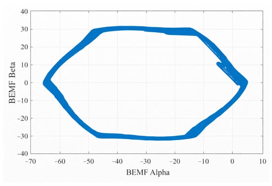
Figure 1. General outline of the waveform of $e_{\alpha }$ vs. $e_{\beta }$.

According to the sensor data, Figure 1 can be redrawn according to the different sector separation logic. The sector parameters of the system are determined and the classification process can be performed. Figure 2 shows the alpha and beta ($\alpha -\beta$) components of the back-EMF for no-load operation divided according to the Hall effect sensor data.

Figure 2. Waveform of $e_{\alpha }$ vs. $e_{\beta }$ according to different sectors for no-load operation.

When the brushless DC motor is under load, the shape of the hexagon starts to rotate according to the load rate. In order to determine the sectors correctly, the mean and variance values of the PDF functions are obtained under different loading conditions. Figure 3 shows the state of the hexagons at different loading conditions.

Figure 3. Waveform of $e_{\alpha }$ vs. $e_{\beta }$ according to different sectors for different load operation.

Using the back-EMF data for a different load operation, the PDF functions of each sector can be illustrated in Figure 4. As can be seen in Figure 4, each Gaussian has a different peak value due to their estimated components in the alpha and beta axes. This ability makes the proposed algorithm more powerful and more flexible than its counterparts due to its parameters being tunable according to the relevant application.

Figure 4. PDF functions behavior graph of brushless DC motor with newly measured data.

The proposed MLE-based commutation sector classifier models the Clarke-transformed back-EMF vector as a two-dimensional Gaussian random variable with a mean that rotates according to the rotor position and scales with electrical speed, while noise and disturbances such as PWM ripple or electromagnetic interference are absorbed into the covariance. The classifier then selects the most likely commutation sector by comparing how close the measured vector is to the expected sector mean, weighted by the variability of the noise. This decision rule is Bayes-optimal under the Gaussian assumption, meaning that it minimizes the probability of misclassification among all possible rules. The reliability of the classifier depends on the statistical separation between the distributions of adjacent commutation sectors. At low speeds, the back-EMF amplitude is small and the separation is narrow, making errors more likely, whereas at higher speeds the separation grows proportionally with the electrical speed and the probability of misclassification rapidly decreases. Load disturbances primarily add constant or slowly varying offsets to the back-EMF vector, which statistically shift the mean and broaden the covariance. If the training or calibration process covers such operating points, the MLE approach continues to provide optimal classification. Parameter inaccuracies such as errors in resistance or inductance values introduce additional bias into the mean or covariance. Robustness is achieved as long as these biases remain smaller than the decision margin, which itself increases with speed and with signal-to-noise ratio. Because most errors occur near sector boundaries, the commutation jitter can be understood as the residual uncertainty between adjacent classes, which becomes negligible once the statistical separation is large enough. Because the mean estimates converge quickly in two dimensions, only modest amounts of training data are needed, and simple online updating rules allow the system to track gradual parameter drift such as that caused by temperature changes. Computationally, the method requires evaluating a small number of arithmetical operations for each classification step (on the order of a hundred additions and multiplications), which is well within the real-time capabilities of low-cost microcontrollers. The simulated system represents a closed-loop speed-controlled BLDC motor drive incorporating a sensorless MLE-based sector determination algorithm. The reference speed is compared with the estimated motor speed to generate a speed error, which is regulated by a PID controller. The PID output defines the duty command used for commutation.

After designating the necessary parameters, the proposed closed loop control scheme can be seen in Figure 5. In Figure 5, $E_{abc}$ denotes the estimated Hall signals. Instead of physical Hall sensors, the commutation logic is driven by the MLE-based sector determination block, which estimates the active electrical sector using the measured three-phase currents $i_{abc}$ and reconstructed back-EMF components $e_{abc}$. Based on the estimated sector, the Hall table generates six-step switching signals for to control the inverter.

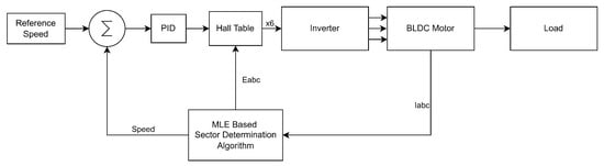
Figure 5. General closed-loop block diagram of the system.

The inverter supplies the BLDC motor, which drives a mechanical load. The motor phase currents are continuously fed back to the MLE algorithm for real-time sector estimation, while the estimated speed is fed back to the outer speed control loop. This structure enables fully sensorless operation while maintaining stable speed regulation and correct commutation.

4.2. Experimental Results

The brushless DC motors have numerous advantages; in addition to these positive sides, however, it has a huge drawback in that it requires an auxiliary control circuit. Eliminating the need for an auxiliary control circuit is possible by using a three-phase inverter. Hence the experimental setup accommodates an inverter, a measurement unit, and a DC generator, which is directly connected to the shaft of the brushless DC motor by a 1:1 speed ratio to simulate the load conditions on the rotor shaft. Figure 6 shows a general view of the experimental setup.

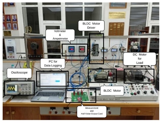
Figure 6. Experimental setup.

The specifications for the brushless DC motor outline key are provided by Table 3. The motor is well-suited for mid-power applications requiring compact, efficient, and responsive operation. The maximum current of 42 A suggests the need for robust power electronics capable of handling high peak loads, especially during acceleration or torque-intensive operations. A maximum speed of 1500 rpm indicates moderate rotational capability, ideal for precision motion control or industrial automation scenarios.

Table 3. Operational parameters of the brushless DC motor.

Max Power	1 kW
Max Speed	1500 rpm
Max Current	42 A
Voltage	24 V
Poles	8

The experimental platform was developed to validate the effectiveness of the proposed sensorless commutation algorithm under realistic operating conditions. The test bench is centered around a brushless DC motor, which is mechanically coupled to a separately excited DC machine used as a controllable load. This arrangement enables the application of variable torque by adjusting the field and armature currents of the DC machine, thereby allowing the brushless DC motor to be tested across a wide range of load conditions. Figure 7 shows the block diagram of experimental setup. In Figure 7, $H_{abc}$ denotes the Hall signals from the motor, while $E_{abc}$ denotes the estimated Hall signals from the algorithm.

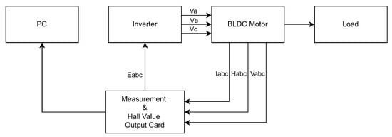
Figure 7. Experimental setup closed-loop block diagram.

The control and signal processing tasks are carried out on a Texas Instruments F28027F LaunchPad digital signal controller (Dallas, TX, USA), which is based on the C2000 family. This platform provides high-speed computational capability, low-latency PWM generation, and integrated peripherals for motor control applications. The use of the F28027F also facilitates seamless interfacing with current sensors, position sensors, and external measurement equipment. Accurate current measurement is essential for both performance evaluation and validation of the proposed estimation algorithm. To this end, a Hall effect-based current sensor is employed. The sensor provides galvanic isolation, wide measurement range, and adequate resolution for capturing both steady-state and transient current dynamics. The measured current signals are fed directly into the ADC channels of the F28027F for real-time processing and monitoring. Figure 8 shows the measurement and Hall value output card detailed view.

Figure 8. Measurement and Hall value output card (detailed view).

For position reference, in the experimental setup the brushless DC motor is equipped with three digital Hall-effect sensors embedded in the stator. These signals are used solely for benchmarking purposes, serving as a reference to evaluate the accuracy of the proposed sensorless commutation method. During the experiments, the Hall sensor outputs were recorded and compared with the algorithm’s estimated commutation signals to quantify deviations. All signals, including phase currents, Hall sensor outputs, and estimated variables, were simultaneously logged using a high-resolution digital oscilloscope and Texas Instruments F28027F LaunchPad digital signal controller. The combination of these tools allowed for detailed observation of back-EMF waveforms, Zero-Crossing Points (ZCPs), commutation instants, and overall current quality. The mechanical speed of the brushless DC motor was monitored indirectly through the coupled DC motor’s voltage output, providing an additional means of validating speed-related performance.

This experimental arrangement ensures that both low-speed and high-speed performance of the proposed algorithm can be evaluated in a controlled manner. The ability to vary load conditions, monitor electrical and mechanical quantities, and compare estimated commutation points with Hall sensor feedback provides a comprehensive validation environment for assessing the robustness, accuracy, and practical applicability of the sensorless control strategy.

In sensorless trapezoidal control methods, it can be said that undoubtedly the most important stage is the determination of the brushless DC motor’s parameters. After the brushless DC motor parameter determination process, rotor position can be estimated by simulating the brushless DC motor model consisting of dynamical equations and motor parameters used to generate the inverter switching signals. These parameters have to be determined in the MLE-based control method as well. The aforementioned motor parameters in the MLE-based method consist of neither phase inductance nor phase resistance. At this point, the meaning of the parameters consists of the sector PDF’s constants such as the class mean and variance. To determine these parameters, the brushless DC motor’s position indication signals are initially run under no-load operation with the help of the ZCPD method; then, PDF parameters for each sector are calculated according to (16) and (17). In Figure 9, measured back-EMF waveforms are shown as blue and zero-crossing points are shown as red, which are the references for position determination under no-load operation.

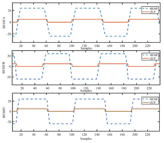
Figure 9. ZCPD-based measured back-EMF waveforms.

As seen in Figure 9, each brushless DC motor has three different phase variables in the time domain. If this concept is evaluated under vector math with the help of vector projection calculation to axes, the number of variables can be reduced from three to two, which is called Clarke transformation. The most important point in the MLE-based method is to decouple the variables from the time. For this purpose, these signals can be plotted against each other to make the process time independent. The $e_{\alpha }$ vs. $e_{\beta }$ graph in Figure 10 is time-independent.

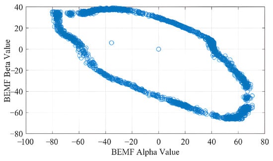
Figure 10. The $e_{\alpha }$ vs. $e_{\beta }$ graph of the brushless DC motor in ZCPD.

The final step in the parameter determination stage can be performed by grouping Figure 10 according to the sensor signals which are obtained from the ZCPD method. Each of the groups corresponds to the value pairs $e_{\alpha }$–$e_{\beta }$ where the rotor is in that region. Due to brushless DC motors having six different sensor value combinations, the number of sectors is six. PDF functions were obtained by calculating each of the discriminated group’s mean and variance values. Figure 11 shows the discriminated $e_{\alpha }$–$e_{\beta }$ graph. In order to examine the behavior of the brushless DC motor with the algorithm developed under load using the parameters obtained after the parameter determination process was completed, the relevant measurements were recorded by applying a reverse load on the DC generator connected to the brushless DC motor shaft. In the first stage, the brushless DC motor was loaded with 0.25 Nm and the current data were recorded. Figure 12 presents the motor phase currents at a load of 0.25 Nm along with the corresponding oscilloscope raw data and ADC-acquired signals. The oscilloscope raw data and the ADC-measured data in Figure 12 are provided together to show the accuracy of the ADC acquisition. The digital measurements used by the proposed algorithm demonstrate that the actual motor signals are faithfully represented. Then, using this current data, the brushless DC motor’s back-EMF voltages can be obtained using the brushless DC motor’s parameters, as shown in Figure 13.

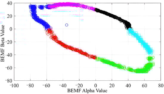
Figure 11. The $e_{\alpha }$ vs. $e_{\beta }$ graph of the brushless DC motor according to sectors (no-load).

Figure 12. Phase current waveforms: (a) oscilloscope raw data and (b) ADC-measured data under 0.25 Nm load.

Figure 13. Measured back-EMF waveform of brushless DC motor under 0.25 Nm load.

Finally, the Clarke transformation of the obtained back-EMF signals is obtained and applied to the each of PDF functions. As a result, the behavior of the PDF functions determined for each sector in Figure 14 under 0.25 Nm load is obtained. Then, the same operations are repeated for 1 Nm load; the related current and back-EMF voltage waveform graphs are given in Figure 15 and Figure 16, respectively. When these collected data are applied to PDF functions, the individual behaviors of the PDF functions for each sector are obtained with the same method, as can be seen in Figure 17. Finally, it can be seen that the probability value of each PDF function is higher than the probability values of other sectors at different times, as demonstrated by Figure 14 and Figure 17.

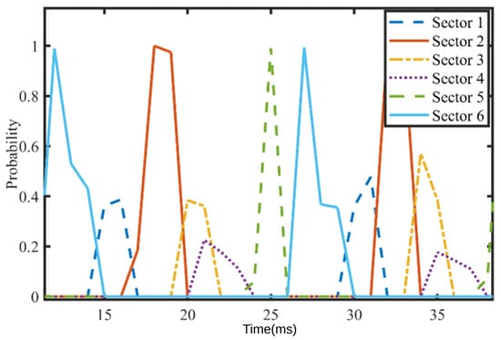
Figure 14. Sector probability density function of brushless DC motor under 0.25 Nm load.

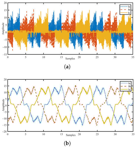
Figure 15. Phase current waveforms: (a) oscilloscope raw data and (b) ADC-measured data under 1 Nm load.

Figure 16. Measured back-EMF waveform of brushless DC motor under 1 Nm load.

Figure 17. Sector probability density function of brushless DC motor under 1 Nm load.

This situation constitutes a suitable statistical background for realizing switching for safe brushless DC motor operation. If the probability value of a sector is higher than other sectors, this clearly shows that the rotor is located in that sector. In addition, when the amount of load is increased, it can be observed that the points where the probability shapes of the sectors intersect are separated with sharper lines. Figure 18 clearly shows that this method outperforms the classical ZCPD method in low-speed and load transition situations. For this reason, based on the obtained results it is convenient to say that the proposed method applies the ZCPD method in a wider speed and load region.

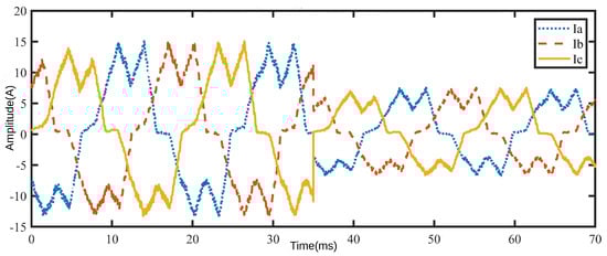
Figure 18. Phase current waveform under load transition (0.25–1 Nm).

The Zero-Crossing Point Detection (ZCPD) method is sensitive to measurement noise due to its strong relation with back-EMF zero-crossing events. Figure 19 shows the sector determination results of two rival methods. Maximum Likelihood Estimation (MLE) uses a statistical framework that accounts for noise characteristics over an observation window, providing significantly higher confidence in noisy operating conditions.

Figure 19. Sector determination results of different methods.

5. Interpretation on Results

5.1. Comparison of the Methods

To better clarify the computational complexity, the computational load of four widely used sensorless brushless DC rotor position estimation methods is compared by counting the Floating Point Operations (FLOPs) per control step. The methods selected are a two-dimensional Gaussian maximum likelihood estimator, zero-crossing point detection, a four-state extended Kalman filter, and a sliding-mode observer. All counts rely on multiplications and additions; divisions, square-roots, and transcendental functions are not included in the FLOP counting procedure.

The Gaussian MLE requires a very modest arithmetical effort. Each class evaluation involves computing the difference between the observation and the class mean, performing a two-by-two matrix–vector multiplication, evaluating a scalar product, and applying a scaling constant. When these operations are counted, roughly thirteen FLOPs per class (or between eighty to one hundred FLOPs in total across six classes) can be obtained. Because the inverse covariance matrices and log determinants can be precomputed offline, runtime complexity remains low, making this method lightweight for embedded implementation.

The zero-crossing detection approach is essentially free from FLOPS. In its simplest form, it relies on sign comparisons, which are integer or logic operations. If a minimal filter is included, such as a first-order Infinite Impulse Response (IIR) applied to one or two channels, the complexity increases slightly to perhaps between eight to sixteen FLOPs per step. From a computational complexity point of view, this method is lightest.

The Extended Kalman Filter (EKF) in a four-state and two-measurement configuration represents the most computationally demanding method among those considered. The prediction step requires a state update and a covariance propagation involving two four-by-four multiplications. The update step of the EKF involves innovation calculation, innovation covariance evaluation, a two-by-two matrix inversion, Kalman gain computation, state correction, and covariance correction. As a result of these steps, the hand-counted FLOPs across these operations amount to approximately 650 to 800 per step. Nonlinear EKFs or sigma-point filters increase the complexity even more.

The sliding-mode or Luenberger-type observer occupies a middle ground. A typical sliding-mode observer includes $\alpha$–$\beta$ Clarke transformation, a linear prediction step, a nonlinear sign or saturation function, error feedback injection, and low-pass filtering of back-EMF estimates. A minimal configuration of this observer may require fifty FLOPs per step; for more realistic versions with filters and gain matrices, the complexity demand of the observer increase to between 150 and 300 FLOPs. This makes observers heavier than MLE, but significantly lighter than EKF.

Among the methods compared in Table 4, the MLE approach stands out as a promising method between computational cost and robustness. With execution times in the range of approximately 50–100$\mathrm{\mu }$s, MLE is well-suited for medium-speed control loops (e.g., <5 kHz) and offers superior classification capabilities, particularly in systems that work at different load conditions. Although not as lightweight as ZCPD or classical observers, MLE provides advantages in noisy environments and systems requiring more precise rotor position estimation.

Table 4. Computational time comparison of brushless DC motor control algorithms.

Method	Typical Time ($\mathbf{\mu }$s)
MLE (2D, 6 classes)	50–100 $\mathrm{\mu }$s
ZCPD	<5 $\mathrm{\mu }$s
Kalman Filter (EKF, 4 states)	200–1000+ $\mathrm{\mu }$s
Observer (e.g., SMO)	20–80 $\mathrm{\mu }$s

For future applications, the MLE method holds substantial potential, especially when combined with modern embedded processing capabilities such as multicore microcontrollers. Real-time implementation of probabilistic models could allow MLE-based controllers to adapt dynamically to changing motor characteristics or load disturbances. Moreover, the development of simplified or hardware-accelerated MLE variants could enable use in higher-frequency control loops, making it a strong candidate for next-generation brushless DC drives in automotive, robotics, and industrial automation applications. Continued research should also explore online training or self-tuning mechanisms for MLE parameters in order to reduce calibration effort and enhance system adaptability over time.

To better position the proposed method within the context of the existing literature, providing a comparative analysis with state-of-the-art sensorless control approaches is important. Conventional Zero-Crossing Detection (ZCPD) methods offer simplicity and low computational cost, but are highly sensitive to noise and typically fail under low-speed conditions. Back-EMF integration techniques improve noise immunity but suffer from phase delay, which can decrease commutation accuracy at medium to high speeds. More advanced approaches such as the Extended Kalman Filter (EKF) provide accurate estimation across a wide operating range but require significant computational resources, which is not feasible for low-cost embedded controllers. High-Frequency Injection (HFI) is effective in the startup region and for low-speed limitations, but increases control complexity and can add additional current harmonics to the system.

In contrast, the proposed MLE-based sector determination method achieves robust commutation in the practical speed range of applications without requiring additional hardware or computationally complex algorithms. Its statistical nature provides resilience against waveform distortions and noise, leading to improved reliability compared to conventional ZCPD or back-EMF integration techniques. MLE has lower complexity than EKF or HFI-based schemes; a summary of the comparative evaluation is provided in Table 5, highlighting the relative advantages and limitations of the proposed method against existing approaches.

Table 5. Comparative analysis of sensorless control methods.

Method	Complexity	Extra Hardware	Low-Speed Capability	Noise Immunity	Suitability for LEVs
Zero-Crossing Detection (ZCPD)	Very low	None	Poor; fails at low speed	Low; distortion-sensitive	Limited; only mid/high speed
Back-EMF Integration	Low	None	Moderate; phase delay	Moderate	Moderate; limited at low speed
Sliding Mode Observer (SMO)	Medium	None	Good; effective from medium to low speed	High; robust to parameter variation	High; widely used, suitable for embedded platforms
Extended Kalman Filter (EKF)	High	None	Good; wide speed range	High	Limited; high computational demand
High-Frequency Injection (HFI)	High	Yes; injection circuit	Excellent; works from standstill	High	Limited; complex and lossy
Proposed MLE-Based Sector Determination	Moderate	None	Moderate; robust after low speed	High; statistical resilience	High; hardware-friendly

One of the limitations of sensorless control methods is their inability to operate at standstill and very low speeds, where the back-EMF signal is not sufficiently high to provide reliable position information. To overcome this issue, a startup strategy is required to enable smooth transition from standstill to the operating region where the proposed sensorless algorithm is effective.

In Section 5.2, an extension of the proposed method will incorporate an open-loop alignment and acceleration strategy. During alignment, the rotor is forced into a known initial position by applying a fixed stator voltage vector. This ensures a deterministic starting point for subsequent commutation. Following alignment, a predefined open-loop commutation sequence is applied to gradually accelerate the motor up to a speed where measurable back-EMF becomes available. When this threshold is reached, the MLE-based sector determination algorithm takes over the control to provide accurate and error-free commutation across the medium and high-speed ranges.

In addition to the above methods, alternative strategies can be considered to enhance robustness. High-frequency signal injection techniques can be used for rotor position estimation based on saliency characteristics; in this way, sensorless operation can be realized at very low speeds. Furthermore, a hybrid scheme employing low-cost Hall sensors or an incremental encoder only for startup, with subsequent switching to full sensorless operation, could also be adopted for practical implementation in light electric vehicles due to safety regulations. These developments remain promising directions for future research aimed at achieving reliable operation across the entire speed spectrum, including startup and low-speed conditions.

5.2. Low Speed Startup Algorithm

In general, sensorless motor drives commonly rely on open-loop startup strategies at standstill and very low speeds to account for the absence of reliable back-EMF information. In open-loop operation, predefined voltage or current vectors are applied to the stator without closed-loop feedback from rotor position or speed estimators. This approach enables the generation of an initial electromagnetic torque that aligns and accelerates the rotor in a controlled manner. Although open-loop startup does not provide rotor position information and may leads to torque oscillations or misalignment under load disturbances, it remains a practical and widely adopted solution for initiating motor motion. To mitigate the inherent uncertainties of open-loop operation, auxiliary techniques such as current-based sector detection or sensitive position estimation are often integrated to detect the rotor’s electrical sector and improve startup reliability. When the rotor reaches a sufficient speed and the signal-to-noise ratio of the observer inputs becomes acceptable, the control system can seamlessly transition from open-loop excitation to closed-loop sensorless control.

6. Conclusions

This study proposes a novel sensorless control method for brushless DC motors based on Maximum Likelihood Estimation (MLE). The proposed approach addresses the limitations of conventional back-EMF zero-crossing techniques. The method utilizes a probability map generated from previously-acquired motor data to improve rotor position estimation accuracy, particularly under noisy conditions.

Compared to traditional zero-crossing detection, the proposed MLE-based approach offers improved noise resilience, prevents rotor locking, and supports reliable commutation over a wider speed range. It also adapts better to load variations, enhancing system robustness in dynamic operating environments.

The results in this paper demonstrate that the proposed method not only increases the efficiency and reliability of the control system but can also enable safer and more stable operation in applications such as electric vehicles and industrial drives in the future. While the use of exponential functions introduces some computational overhead, future work will focus on optimizing this aspect for real-time embedded applications.

References

- Kim, T.-H.; Ehsani, M. Sensorless control of the BLDC motors from near-zero to high speeds. IEEE Trans. Power Electron. 2004, 19, 1635–1645. [Google Scholar] [CrossRef]
- Shao, J.; Nolan, D.; Teissier, M.; Swanson, D. A novel sensorless brushless DC (BLDC) motor drive for automotive fuel pumps. In Proceedings of the Power Electronics in Transportation, Auburn Hills, MI, USA, 24–25 October 2002; pp. 53–59. [Google Scholar]
- Pillai, N.S.; Vipin, A.M.; Radhakrishnan, R. Analysis and simulation studies for position sensorless BLDC motor drive with initial rotor position estimation. In Proceedings of the 2015 International Conference on Nascent Technologies in the Engineering Field (ICNTE), Navi Mumbai, India, 9–10 January 2015; pp. 1–6. [Google Scholar]
- Buchnik, Y.; Rabinovici, R. Speed and position estimation of brushless DC motor in very low speeds. In Proceedings of the 2004 23rd IEEE Convention of Electrical and Electronics Engineers in Israel, Tel-Aviv, Israel, 6–7 September 2004; pp. 317–320. [Google Scholar]
- Shao, J.; Nolan, D.; Hopkins, T. A novel direct back EMF detection for sensorless BLDC motor drives. In Proceedings of the APEC. Seventeenth Annual IEEE Applied Power Electronics Conference and Exposition, Dallas, TX, USA, 10–14 March 2002; Volume 1, pp. 33–37. [Google Scholar]
- Shao, J.; Nolan, D.; Hopkins, T. Improved direct back EMF detection for sensorless BLDC motor drives. In Proceedings of the Eighteenth Annual IEEE Applied Power Electronics Conference and Exposition, APEC ’03, Miami Beach, FL, USA, 9–13 February 2003; Volume 1, pp. 300–305. [Google Scholar]
- Jin, H.; Liu, G.; Li, H.; Chen, B.; Zhang, H. A fast commutation error correction method for sensorless BLDC motor considering rapidly varying rotor speed. IEEE Trans. Ind. Electron. 2021, 69, 3938–3947. [Google Scholar] [CrossRef]
- Zhang, H.; Li, H. Fast commutation error compensation method of sensorless control for MSCMG BLDC motor with nonideal back EMF. IEEE Trans. Power Electron. 2020, 36, 8044–8054. [Google Scholar] [CrossRef]
- Veeramsetty, V.; Edudodla, B.R.; Salkuti, S.R. Zero-crossing point detection of sinusoidal signal in presence of noise and harmonics using deep neural networks. Algorithms 2021, 14, 329. [Google Scholar] [CrossRef]
- Park, M.; Sohn, S.-m.; Kwon, D.-S. High-reliable sensorless positioning of BLDC motor using mutation programming. IEEE Trans. Veh. Technol. 2022, 71, 1643–1654. [Google Scholar]
- Wang, Y.; Chen, S.; Liu, Z. A back-EMF based machine learning approach for accurate commutation timing in sensorless BLDC motors. IEEE Trans. Ind. Inf. 2023, 19, 4567–4576. [Google Scholar]
- Kim, T.-H.; Ehsani, M. An error analysis of the sensorless position estimation for BLDC motors. In Proceedings of the 38th IAS Annual Meeting on Conference Record of the Industry Applications Conference, Salt Lake City, UT, USA, 12–16 October 2003; Volume 1, pp. 611–617. [Google Scholar]
- Chen, L.; He, Y.; Zhao, M. Deep learning-based sensorless torque and position estimation for high-performance BLDC drives. IEEE J. Emerg. Sel. Topics Power Electron. 2024, early access. [Google Scholar]
- Soni, U.K.; Tripathi, R.K. Sensorless control of high-speed BLDC motor using equal area criterion based precise commutation scheme with fuzzy based phase delay compensation. Int. Trans. Electr. Energy Syst. 2021, 31, e13001. [Google Scholar] [CrossRef]
- Reuben, J.; Onah, C.O.; Agber, J.U. Modeling and simulation of three phase induction motor electrical faults using MATLAB/Simulink. Int. J. Mod. Trends Eng. Res. (IJMTER) 2018, 5, 176–187. [Google Scholar]
- Balogh, T.; Fedak, V.; Durovský, F. Modeling and simulation of the BLDC motor in MATLAB GUI. In Proceedings of the 2011 IEEE International Symposium on Industrial Electronics, Gdansk, Poland, 27–30 June 2011; pp. 1403–1407. [Google Scholar]
- Kelek, M.M.; Çelik, İ.; Fidan, U.; Oğuz, Y. The simulation of mathematical model of outer rotor BLDC motor. SETSCI Conf. Proc. 2019, 9, 412–415. [Google Scholar]
- Rao, A.P.C.; Obulesh, Y.P.; Babu, C.S. Mathematical modeling of BLDC motor with closed loop speed control using PID controller under various loading conditions. ARPN J. Eng. Appl. Sci. 2012, 7, 1321–1328. [Google Scholar]
- Millar, R.B. Maximum Likelihood Estimation and Inference: With Examples in R, SAS and ADMB; Wiley: Hoboken, NJ, USA, 2011. [Google Scholar]
- Le Cam, L. The central limit theorem around 1935. Statist. Sci. 1986, 1, 78–91. [Google Scholar]
- Cowan, G. Statistical Data Analysis; Lecture Notes; Royal Holloway University: London, UK, 2025; Available online: https://www.pp.rhul.ac.uk/~cowan/stat/stat_5.pdf (accessed on 14 May 2025).
- Pan, J.-X.; Fang, K.-T. Maximum likelihood estimation. In Growth Curve Models and Statistical Diagnostics; Springer: New York, NY, USA, 2002; pp. 77–158. [Google Scholar]
- Abdulali, B.A.A.; Bakar, M.A.A.; Ibrahim, K.; Ariff, N.M. Extreme value distributions: An overview of estimation and simulation. J. Probab. Stat. 2022, 2022, 5449751. [Google Scholar] [CrossRef]
- Purcell, S. Maximum Likelihood Estimation. 2007. Available online: http://statgen.iop.kcl.ac.uk/bgim/mle/sslike_3.html (accessed on 20 December 2024).
- O’Rourke, C.J.; Qasim, M.M.; Overlin, M.R.; Kirtley, J.L. A geometric interpretation of reference frames and transformations: dq0, Clarke, and Park. IEEE Trans. Energy Convers. 2019, 34, 2070–2083. [Google Scholar] [CrossRef]
- Astrachan, O. Bubble sort: An archaeological algorithmic analysis. ACM SIGCSE Bull. 2003, 35, 1–5. [Google Scholar] [CrossRef]
Disclaimer/Publisher’s Note: The statements, opinions and data contained in all publications are solely those of the individual author(s) and contributor(s) and not of MDPI and/or the editor(s). MDPI and/or the editor(s) disclaim responsibility for any injury to people or property resulting from any ideas, methods, instructions or products referred to in the content. |
© 2025 by the authors. Licensee MDPI, Basel, Switzerland. This article is an open access article distributed under the terms and conditions of the Creative Commons Attribution (CC BY) license.