Fuzzy Adaptive Impedance Control Method for Underwater Manipulators Based on Bayesian Recursive Least Squares and Displacement Correction

Abstract

During constant-force operations in complex marine environments, underwater manipulators are affected by hydrodynamic disturbances and unknown, time-varying environment stiffness. Under classical impedance control (IC), this often leads to large transient contact forces and steady-state force errors, making high-precision compliant control difficult to achieve. To address this issue, this study proposes a Bayesian recursive least-squares-based fuzzy adaptive impedance control (BRLS-FAIC) strategy with displacement correction for underwater manipulators. Within a position-based impedance-control framework, a Bayesian Recursive Least Squares (BRLS) stiffness identifier is constructed by incorporating process and measurement noise into a stochastic regression model, enabling online estimation of the environment stiffness and its covariance under noisy, time-varying conditions. The identified stiffness is used in a displacement-correction law derived from the contact model to update the reference position, thereby removing dependence on the unknown environment location and reducing steady-state force bias. On this basis, a three-input/two-output fuzzy adaptive impedance tuner, driven by the force error, its rate of change, and a stiffness-perception index, adjusts the desired damping and stiffness online under amplitude limitation and first-order filtering. Using an underwater manipulator dynamic model that includes buoyancy and hydrodynamic effects, MATLAB simulations are carried out for step, ramp, and sinusoidal stiffness variations and for planar, inclined, and curved contact scenarios. The results show that, compared with classical IC and fuzzy adaptive impedance control (FAIC), the proposed BRLS-FAIC strategy reduces steady-state force errors, shortens force and position settling times, and suppresses peak contact forces in variable-stiffness underwater environments.

1. Introduction

With the continuous development of marine resource utilization and underwater operation technologies, underwater manipulators and other subsea robotic systems have become crucial equipment for performing complex tasks, and are widely employed in underwater exploration and inspection, deep-sea specimen collection, and hull and infrastructure maintenance [1,2,3]. Vision- and learning-based methods have also been introduced to enhance environment perception and task execution, including image-recognition-based grasp control for manipulators and deep-learning-based optical remote sensing scene classification for representing large-scale ocean scenes and providing prior information for marine operations [4,5]. However, such sensing capabilities do not change the physical interaction between the manipulator and its environment. When the end-effector comes into contact with its surroundings, hydrodynamic effects-such as fluid added mass, viscous drag, buoyancy, and flow-induced disturbances-together with unknown, time-varying environment stiffness, readily give rise to force fluctuations and pose deviations, thereby degrading operational stability and task accuracy. Consequently, achieving stable and compliant control under these conditions has become one of the key challenges in underwater manipulation [6]. Compliant control aims to maintain appropriate compliance during interaction so that the manipulator can track the desired motion stably while avoiding excessive contact forces that may cause damage. Among various approaches, impedance control is a representative paradigm: by establishing a dynamic relationship involving mass, damping, and stiffness between the desired and actual interaction forces, it enables coordinated position-force regulation. Impedance control has been widely applied in industrial assembly, medical procedures, and service robotics, for example by adjusting parameters to accommodate different assembly tolerances or by enhancing safety and comfort in human–robot interaction [7,8,9].

To address contact control in complex environments, many studies have concentrated on impedance control [10,11,12,13,14,15] and admittance control [16,17,18,19]. Gu et al. [20] proposed a fractional-order Proportional-Integral-Derivative (PID) adaptive impedance control strategy for unknown environment force tracking, in which environment parameters are estimated online within a classical impedance framework to generate reference trajectories and reduce force error; a fractional-order PID controller is further employed to enhance model adaptability and transient performance, and closed-loop stability is proven. Simulation results indicate that, compared with several impedance-based baseline methods, this strategy achieves superior robustness and faster convergence; however, its performance is sensitive to the selection of fractional orders and gains, and improper tuning may lead to longer settling times or larger steady-state errors. Zheng et al. [21] developed a fuzzy adaptive sliding-mode impedance control scheme for reset robots, where a force-residual observer enables sensorless end-effector force estimation, inverse dynamics combined with Proportional-Derivative control is used for system linearization, and a sliding-mode robust term together with a fuzzy adaptive switching gain is introduced to suppress chattering. Simulations show that the method outperforms comparative strategies in both position and force tracking; nevertheless, it remains sensitive to initial conditions and model accuracy, and large estimation or modeling errors may cause inappropriate gain scheduling and slower convergence. Khan et al. [22] proposed an end-effector force-tracking method for nuclear-power-plant dismantling, employing impedance control driven by super-twisting sliding-mode control (STSMC) and tuning the parameters via particle swarm optimization (PSO); comparative studies demonstrate smoother and more robust force tracking under uncertainties. However, the performance is influenced by the gain and constraint settings of STSMC and PSO, and inadequate tuning can degrade chattering suppression and convergence. Fu et al. [23] presented an optimization-based variable-impedance control approach for medical contact tasks, in which the optimal stiffness is obtained via online quadratic programming and a passivity-ensuring energy tank is introduced. Experiments show better force tracking and consistency than fixed-stiffness control and manual operation, but the method is sensitive to cost weights and constraints, and its real-time capability and stability margins may be limited in fast or strongly noisy scenarios.

However, compared with terrestrial environments, the underwater environment exhibits stronger nonlinearity and uncertainty. Conventional impedance control is difficult to effectively cope with variations in environmental stiffness and hydrodynamic disturbances, often leading to large steady-state force errors and oscillatory transient responses. To address these issues, extensive studies have been conducted and various improved strategies have been proposed. Zhang et al. [24] developed a model-reference adaptive impedance control method for underwater manipulators with model uncertainties. By introducing a desired impedance model and a bounded-gain forgetting adaptive law, coordinated convergence of end-effector force and position is achieved. Simulation results demonstrate good robustness and stability under uncertain dynamics; however, the performance is sensitive to the selection of the reference model and forgetting gains, and improper tuning may result in slower convergence or increased steady-state bias. For multi-objective grasping tasks of underwater manipulators, Zhang et al. [25] proposed an adaptive impedance control scheme. Within a position-based impedance framework, impedance parameters are identified online via Recursive Least Squares (RLS), and the desired force and desired position are jointly adjusted to realize compliant force control and reduce steady-state error. Nevertheless, this method relies heavily on the accuracy and latency of online identification; under rapidly time-varying or strongly noisy conditions, estimation errors can propagate to the coupled regulation of desired force and position, thereby degrading tracking performance. Lu et al. [26] proposed two force-tracking schemes for compliant grasping: an identification-based impedance controller that updates the environment stiffness online using a forgetting-factor RLS, and an adaptive impedance controller that adjusts the target stiffness and desired position with additional compensation terms. Simulation and real underwater experiments show that the former is less sensitive to the response speed of the inner position loop and exhibits better robustness, but it strongly depends on identification quality and the choice of forgetting factor, so that under strong noise or rapidly changing environments parameter lag may occur and reduce stability margins. Yu et al. [27] presented a robust impedance-control method for constant contact-force regulation, in which a virtual control input is introduced into the impedance framework and combined with sliding-mode control and a disturbance observer to enhance disturbance rejection and contact-force accuracy. Simulations under various seabed conditions indicate that this method can effectively suppress contact-force fluctuations and improve motion stability. However, its performance is sensitive to the modeling of seabed uncertainties and the tuning of observer parameters; when seabed geometry or medium properties change rapidly and measurement noise increases, disturbance estimation tends to lag, thereby deteriorating constant-force accuracy and stability margins. Dai et al. [28] applied sliding-mode impedance control to I-AUV contact intervention, realizing integrated force-position control from non-contact to contact phases. Simulations and full-scale/bench experiments that account for model uncertainties and hydrodynamic disturbances verify good tracking performance in both position and contact force, supporting offshore maintenance and related tasks. Nevertheless, the method is sensitive to sliding-mode gains, switching-layer thickness, and the timing of phase transitions; in the presence of sensor noise and time delays, its chattering-suppression capability and stability margins are still limited.

However, despite the above advances, existing approaches still exhibit several limitations. First, the characterization of time-varying environment stiffness is often inadequate, and the impedance parameters cannot adapt promptly under abrupt changes, linear drifts, or periodic variations. Second, disturbance and noise handling typically relies on fixed gains or offline parameter tuning, which leads to fluctuating stability margins under varying operating conditions. Third, the lack of a unified mechanism for parameter updating and safety constraints may cause overshoot, oscillations, and steady-state errors during rapid contact transitions. From a broader perspective, learning-based policy optimization has also been explored for contact regulation, with deep reinforcement learning controllers such as DDPG and TD3 being representative examples. Comparisons against such policies could provide a complementary baseline and help further contextualize the interpretability and safety-constrained tuning advantages of the proposed controller under contact uncertainties [29].

Based on the above analysis, this paper develops a BRLS-FAIC scheme with displacement correction for underwater manipulators. The main contributions are summarized as follows:

• A BRLS stiffness identifier is embedded into a position-based impedance-control framework. By explicitly modeling process and measurement noise within a stochastic regression model and updating the parameter covariance via a prediction-correction mechanism, the proposed BRLS estimator provides noise-robust, real-time environment-stiffness estimates under both slowly and rapidly varying conditions, without relying on heuristic tuning of forgetting factors.
• A novel displacement-correction mechanism is derived from the end-effector-environment contact model and integrated into the reference-trajectory generation. The stiffness identified by BRLS is used to reconstruct the effect of the unmeasured environment position and to compensate the reference displacement, thereby removing the explicit dependence of the steady-state force error on the unknown contact location. In addition, a linear feedforward term based on the force error is incorporated to mitigate large position steps at stiffness jumps and contact onset, improving constant-force regulation and reducing transient impact forces.
• A stiffness-aware fuzzy adaptive impedance tuner with three inputs and two outputs is designed to coordinate damping and stiffness adaptation. Using the force error, its time derivative, and a normalized stiffness-perception index as inputs, the tuner adjusts the desired damping and stiffness online under amplitude limitation and first-order filtering, achieving a trade-off between peak-force suppression, transient response speed, and steady-state tracking accuracy across soft-hard environment transitions and planar, inclined, and curved contact geometries.

2. Materials and Methods

2.1. Dynamic Modeling and Analysis of an Underwater Manipulator

Dynamic modeling provides a foundation for analyzing the motion behavior and control properties of manipulators. Common modeling approaches include the Lagrange method, the Newton–Euler method, and the Kane method, and an appropriate formulation can be selected according to the manipulator structure, number of degrees of freedom, and analysis objectives. In this paper, a systematic model of the underwater manipulator is developed based on the Lagrangian dynamics framework [30,31].

When hydrodynamic effects are neglected, the joint-space dynamics of the manipulator can be expressed as follows:

$$M(q)\ddot{q}+C(q,\dot{q})\dot{q}+G(q)={\tau }_m-{\tau }_f-{\tau }_e$$

(1)

where $M(q)$ is the inertia matrix; $C(q,\dot{q})$ is the Coriolis and centrifugal matrix; $G(q)$ represents the generalized gravity, including the combined effects of gravity and buoyancy; ${\tau }_m$, ${\tau }_f$, and ${\tau }_e$ denote the actuator driving torque, joint friction torque, and interaction torque between the end-effector and the environment, respectively; and $q$, $\dot{q}$, $\ddot{q}$ are the joint position, velocity, and acceleration.

In an underwater environment, the motion of the underwater manipulator is influenced by hydrodynamic effects such as added mass, hydrodynamic drag, and buoyancy. For modeling and analysis convenience, the combined effect of gravity and buoyancy is represented by an equivalent gravity term [32]. According to hydrostatic theory, this equivalent gravity can be expressed as:

$$G_{eq}=G-F_b=mg-{\rho }_{w}gV=mg(1-{\displaystyle \frac{{\rho }_w}{{\rho }_r}})$$

(2)

where $m$ is the mass of the manipulator, $V$ is the volume of water displaced by the manipulator, ${\rho }_w$ and ${\rho }_r$ are the water density and the material density of the manipulator, respectively, and $g$ denotes the gravitational acceleration. Equation (2) shows that buoyancy partially counteracts gravity, thereby reducing the equivalent gravitational load of the system.

In addition, underwater motion is subject to significant hydrodynamic loads, mainly including inertial effects induced by added mass and velocity-dependent fluid drag [33]. The corresponding hydrodynamic torque can be expressed as:

$${\tau }_h={\tau }_d+{\tau }_i$$

(3)

where ${\tau }_i$ denotes the inertial torque induced by the added-mass effect and ${\tau }_d$ denotes the fluid-drag torque associated with the joint velocity. Together, they represent the additional load exerted by the fluid on the manipulator.

By substituting Equations (2) and (3) into Equation (1), the dynamic equation of the underwater manipulator can be written as:

$$M(q)\ddot{q}+C(q,\dot{q})\dot{q}+G_{eq}(q)={\tau }_m-{\tau }_f-{\tau }_e-{\tau }_h$$

(4)

Equation (4) describes the joint-space motion of the manipulator in an underwater environment under the combined effects of inertia, buoyancy, friction, and hydrodynamic forces.

Compared with a joint-space formulation, a task-space representation provides a more direct description of end-effector motion and interaction forces [34]. The relationship between the end-effector linear velocity and the joint velocity can be expressed as:

$$\dot{x}=J(q)\dot{q}$$

(5)

where $J(q)$ denotes the Jacobian matrix. According to the principle of coordinate transformation, the above equation can be rewritten in the task-space form as:

$$M_x(q)\ddot{x}+C_x(q,\dot{q})\dot{x}+G_x(q)=F_m-F_f-F_e-F_h$$

(6)

where $M_x$, $C_x$ and $G_x$ denote the equivalent inertia matrix, the Coriolis/centrifugal term, and the equivalent gravity term in the task space, respectively, while $F_m$, $F_f$, $F_e$ and $F_h$ represent the driving force, friction force, environmental interaction force, and hydrodynamic force, respectively. Since the subsequent impedance and force control laws are designed in the task space, Equation (6) is used as the basic model for controller derivation, and the explicit expressions of each term are omitted for brevity.

2.2. Position-Based Impedance Control

Impedance control is a typical compliant control approach that models the manipulator as a virtual mass-spring-damper system, enabling the robot to generate appropriate motion responses to external forces and thereby realize compliant interaction and force regulation. According to different control objectives, impedance control can be classified into position-based and force-based schemes. In position-based impedance control, the contact force is adjusted indirectly by regulating the desired end-effector position, and a virtual spring-damper relationship is established using position and velocity errors, so that compliant modulation of the end-effector motion is achieved in task space [35,36]. A one-dimensional representation of the desired impedance is shown in Figure 1.

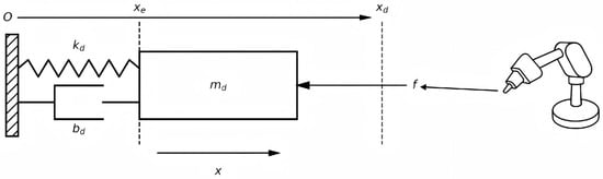
Figure 1. One-dimensional mass-spring-damper impedance model.

For simplicity of analysis, this study considers only the one-dimensional motion of the end-effector along the normal contact direction. This simplifying assumption does not affect the generality of the results, since the same modeling form and control law can be applied to each axis of a multi-degree-of-freedom system [37]. In practical multi-DOF contact, cross-axis coupling induced by kinematics and contact geometry may generate tangential-normal interactions, so that the effective stiffness perceived along a nominal contact direction can be influenced by motion in other axes. Under such conditions, a full task-space implementation with matrix impedance and coupling-aware stiffness processing can reduce performance degradation; otherwise, cross-axis effects enter the outer loop as additional bounded perturbations and may mainly appear as increased transient force ripple or slower convergence. Let $x$ denote the actual position of the end-effector and $f$ denote the actual contact force at the end-effector. Then, the position-based impedance control model can be expressed as:

$$m_d(\ddot{x}-{\ddot{x}}_d)+b_d(\dot{x}-{\dot{x}}_d)+k_d(x-x_d)=f-f_d$$

(7)

where $m_d$, $b_d$ and $k_d$ denote the desired mass, desired damping, and desired stiffness parameters of the impedance model, respectively; $x$, $\dot{x}$ and $\ddot{x}$ represent the actual position, velocity, and acceleration of the end-effector; $x_d$, ${\dot{x}}_d$ and ${\ddot{x}}_d$ represent the desired position, velocity, and acceleration of the end-effector; $f$ and $f_d$ denote the actual and desired contact forces at the end-effector, respectively.

The environment stiffness is denoted by $k_e$ and the environment position by $x_e$. When the end-effector is in contact with the environment, the contact-force model can be expressed as:

$$f=\left\{\begin{array}{l}{k}_e(x-x_e)\\ 0\end{array}\right.\begin{array}{l},x\ge x_e\\ ,x<x_e\end{array}$$

(8)

When the steady-state error is zero, the actual contact force satisfies $f=f_d$, and the steady-state force error ${\mathrm{e}}_{fss}=f-f_d$ can be derived from the impedance model in Equation (7) as:

$$e_{fss}=f-f_d={\displaystyle \frac{k_d}{k_d+k_e}}\left[k_e(x_d-x_e)-f_d\right]$$

(9)

In practical operation environments, the equivalent stiffness $k_e$ is typically unknown and time-varying, while the environment position $x_e$ is also difficult to measure directly. Equation (9) indicates that the steady-state force error $e_{fss}$ depends on the stiffness $k_e$ and environment position $x_e$ as well as the chosen reference position $x_d$. Therefore, to eliminate the steady-state force error, the reference position should be chosen as:

$$x_d=x_e+{\displaystyle \frac{f_d}{k_e}}$$

(10)

That is, if the environment stiffness $k_e$ and environment position $x_e$ were known and remained constant, adopting this reference position would guarantee zero steady-state force error. In practical applications, however, these conditions are rarely satisfied simultaneously, and fixed impedance parameters usually cannot ensure zero steady-state error; unavoidable residual bias arises due to uncertainties in environment stiffness and contact location. Therefore, the remainder of this paper focuses on online identification of the environment stiffness and the treatment of environment-position uncertainty, and, on this basis, develops a displacement-correction strategy to reduce the steady-state force error.

Based on the above analysis, the block diagram of the impedance-control scheme can be constructed, as illustrated in Figure 2. In this structure, a position controller is placed in the inner loop and a force-control loop is arranged outside; the contact force is regulated indirectly by adjusting the displacement compensation at the end-effector. In the diagram, $x_d$ denotes the desired position, $x_r$ denotes the reference position after displacement correction, $x$ is the actual position, ${\mathrm{e}}_x$ and ${\mathrm{e}}_f$ are the position and force errors, respectively, $f_d$ denotes the desired contact force, $f$ is the actual contact force, and $△x$ is the displacement compensation generated by the impedance controller. The position controller is typically implemented using a PID algorithm to ensure system stability and satisfactory tracking performance. This structure has been widely adopted in studies on compliant control and provides the basis for the subsequent design of adaptive and fuzzy controllers.

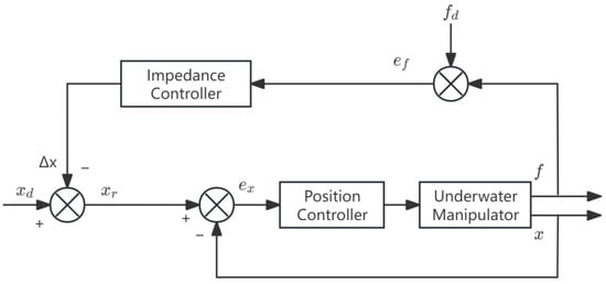
Figure 2. Position based impedance control block diagram.

3. Parameter Identification and Novel Displacement Correction Based on Bayesian Recursive Least Squares

3.1. Recursive Least Squares Method

Recursive least squares (RLS) is a commonly used adaptive estimation algorithm for online parameter identification. By updating parameter estimates recursively using streaming input-output data, RLS enables real-time tracking of time-varying characteristics [38]. Compared with conventional batch least-squares estimation, the recursive formulation features low per-sample computational cost and fast updates, and has therefore been widely applied to robotic force control and environment-parameter identification.

When the manipulator performs planar constant-force tracking tasks, the environment stiffness $k_e$ directly affects the steady-state performance of impedance control. According to the previous dynamic and impedance analysis, the steady-state force error is directly related to $k_e$ and to the environment-position mismatch. In hard-contact scenarios, if $k_e$ and $x_e$ are not explicitly treated, the force-tracking error will be significantly amplified. To achieve accurate constant-force tracking under unknown or time-varying stiffness, an online parameter-identification and displacement-correction strategy is introduced within the impedance framework. The environment stiffness $k_e$ is estimated in real time using an RLS method, and the contact model is exploited to transform $x_e$ into a function of measurable quantities and $k_e$, thereby removing the explicit dependence on $x_e$ in the generation of the reference position.

A general linear regression model can be written as:

$$y_k={\varphi }_k^{\top }\theta +v_k$$

(11)

Based on this model, a weighted least-squares criterion with a forgetting factor $\lambda \in (0.95,1]$ is adopted, whose cost function is defined as:

$$J_k(\theta )={\displaystyle \sum _{i=1}^k{\lambda }^{k-i}}{\left(y_i-{\varphi }_i^{\top }\theta \right)}^2$$

(12)

where $\lambda$ denotes the forgetting factor used to attenuate the weights of past samples, $y_k$ denotes the measured output, ${\varphi }_k$ denotes the regression vector, and $\theta$ denotes the parameter vector to be estimated.

The standard recursive form of the RLS algorithm can be written as:

$$\left\{\begin{array}{l}{K}_k={\displaystyle \frac{P_{k-1}{\varphi }_k}{\lambda +{\varphi }_k^{\top }{P}_{k-1}{\varphi }_k}}\\ {\widehat{\theta }}_k={\widehat{\theta }}_{k-1}+K_k\left(y_k-{\varphi }_k^{\top }{\widehat{\theta }}_{k-1}\right)\\ P_k={\lambda }^{-1}\left(P_{k-1}-K_k{\varphi }_k^{\top }{P}_{k-1}\right)\end{array}\right.$$

(13)

where $P_k$ denotes the covariance matrix and $K_k$ denotes the gain matrix. The algorithm has a simple structure and a low computational burden, and it is capable of providing real-time estimates of the environment stiffness. In the subsequent stiffness-identification scheme, $y_k$ is taken as the force increment, ${\varphi }_k$ as the displacement increment, and $\theta$ as the environment stiffness.

3.2. Bayesian Recursive Least Squares (BRLS)

When the environment stiffness varies abruptly or the measurement noise is significant, the conventional RLS algorithm with a fixed forgetting factor tends to suffer from estimation lag or oscillation. To improve the adaptability of the algorithm in non-stationary environments, adaptive forgetting factors have been introduced in existing studies, where the forgetting factor is adjusted online according to the signal error so as to accelerate the update when the error is large and to maintain smooth estimates when the error is small.

In contrast to the above approaches that rely on tuning the forgetting factor, this paper develops a BRLS algorithm from a Bayesian estimation perspective, aiming to further enhance the stability and dynamic response of stiffness identification. In the proposed method, process noise and measurement noise are explicitly modeled within the conventional RLS framework, and the covariance matrix is updated through an adaptive prediction-correction mechanism, thereby improving the robustness of parameter estimation under complex noise conditions without additional dependence on a forgetting factor. Specifically, BRLS performs a covariance prediction driven by the assumed process-noise variance ${\sigma }_w^2(k)$, and then applies a covariance correction using the current innovation together with the measurement-noise variance ${\sigma }_v^2(k)$, following the standard Bayesian recursion. In this sense, the update is inherently adaptive: the gain $K(k)$ in Equation (16) is data-dependent and varies online with the current excitation $\varphi (k)$, the predicted covariance, and the innovation level, thereby accelerating parameter tracking when informative increments are present while remaining conservative under low excitation or noisy measurements to suppress estimation jitter.

The stiffness identification is formulated through an incremental force-displacement relation, in which the unknown stiffness appears linearly as a regression coefficient. This structure naturally motivates a least-squares recursion, while BRLS further propagates parameter uncertainty through a Bayesian prediction-correction update. EKF-type joint estimation and adaptive-observer formulations provide a general route for parameter adaptation, but they are typically tied to an explicit nonlinear state-space description and associated model-based design choices, which increases implementation complexity and places stronger requirements on model fidelity. In contrast, BRLS matches the incremental regression structure adopted here and yields a lightweight estimator with an explicit covariance update, thereby facilitating stable stiffness tracking and seamless integration with the displacement-correction loop.

The present identification focuses on stiffness as the dominant contact property and adopts a quasi-static incremental relation. If environment dynamics such as relative-velocity-dependent damping are explicitly included, the measurement relation must be augmented with additional parameters and a richer excitation is generally required to maintain reliable separation between stiffness and damping effects. Under such augmentation, the BRLS recursion remains applicable in principle, while the estimator order and the tuning of process and measurement covariances would need to be adjusted to preserve stable convergence.

To characterize the time-varying nature of the environment stiffness, the parameter to be identified is modeled as a stochastic process, and its state evolution and measurement relations are expressed as:

$$\left\{\begin{array}{l}\theta (k)=\theta (k-1)+w(k-1)\\ y(k)={\varphi }^T(k)\theta (k)+v(k)\end{array}\right.$$

(14)

where $\theta (k)$ denotes the stiffness parameter at the k-th sampling instant, $\varphi (k)$ denotes the regression vector, $y(k)$ denotes the measured output, and $w(k)$ and $v(k)$ denote the process noise and measurement noise, respectively. Both noise terms are assumed to be zero-mean Gaussian white noise, i.e.:

$$\left\{\begin{array}{l}w(k)~\mathcal{N}\left(0,{\sigma }_w^2(k)\right)\\ v(k)~\mathcal{N}\left(0,{\sigma }_v^2(k)\right)\end{array}\right.$$

(15)

where ${\sigma }_w^2(k)$ and ${\sigma }_v^2(k)$ denote the variances of the process noise and the measurement noise, respectively. In underwater measurements, occasional outliers may violate the Gaussian assumption and yield large innovations, which can introduce transient bias in the stiffness update.

When the force measurement is severely corrupted, the innovation can be dominated by measurement fluctuations and the stiffness update becomes less informative; in such cases, conservative signal conditioning together with update gating can help maintain stable tracking performance. Under these assumptions, the recursive form of the BRLS algorithm can be derived based on Bayesian recursion as follows:

$$\left\{\begin{array}{ll}P(k|k-1)=P(k-1)+{\sigma }_w^2(k)\hfill & \hfill \\ K(k)={\displaystyle \frac{P(k|k-1)\varphi (k)}{{\varphi }^T(k)P(k|k-1)\varphi (k)+{\sigma }_v^2(k)}}\hfill & \hfill \\ e(k)=y(k)-{\varphi }^T(k)\widehat{\theta }(k-1)\hfill & \hfill \\ \widehat{\theta }(k)=\widehat{\theta }(k-1)+K(k)e(k)\hfill & \hfill \\ P(k)=P(k|k-1)-K(k){\varphi }^T(k)P(k|k-1)\hfill & \hfill \end{array}\right.$$

(16)

where $\widehat{\theta }(k)$ denotes the parameter estimate at the k-th sampling instant, $e(k)$ denotes the current measurement residual, and $P(k)$ denotes the parameter covariance matrix. By appropriately selecting and adaptively tuning ${\sigma }_w^2(k)$ and ${\sigma }_v^2(k)$ according to the residual information, the BRLS algorithm maintains estimation stability while significantly enhancing its tracking capability for time-varying stiffness, thereby providing more accurate and robust environment-stiffness information for the subsequent displacement correction and online impedance-parameter adjustment.

From an implementation perspective, RLS, AF-RLS, and BRLS share the same incremental regression structure in this work and therefore admit lightweight online updates. Since the identified parameter is scalar stiffness, the per-sample computations reduce to a small number of arithmetic operations, and BRLS only adds a simple covariance prediction–correction step without changing the order of complexity. When extended to a parameter vector of dimension n, the dominant cost is the covariance update, which scales quadratically in $n$ in both time and memory.

3.3. Novel Displacement Correction Scheme

To utilize the online-identified environment stiffness for constant-force tracking control, a reference-trajectory generation mechanism that ensures consistency between force and displacement needs to be incorporated into the impedance-control framework. When impedance control is employed to achieve constant-force output, if the desired position is not adjusted according to the variation of environment stiffness, significant steady-state force bias may occur under hard-contact conditions, and even instability may be induced. Therefore, based on the aforementioned BRLS-based stiffness identification, a displacement-correction scheme is developed that balances steady-state accuracy and dynamic performance.

Assuming that the end-effector undergoes elastic contact along the normal direction and that the zero steady-state error condition is satisfied, the relationship between the contact force and the environment position can be described by a linear contact model, which is expressed as:

$$\left\{\begin{array}{l}f=k_e(x-x_e)\\ x_d=x_e+{\displaystyle \frac{f_d}{k_e}}\end{array}\right.$$

(17)

Although Equation (17) adopts a linear stiffness form for derivation, the proposed framework is not restricted to strictly linear media. For contacts exhibiting nonlinear compression, the identified stiffness can be interpreted as an equivalent incremental stiffness over each sampling interval, so that the same incremental force-displacement regression and BRLS recursion remain applicable as a local update. In this sense, the controller operates on a time-varying tangent stiffness, while pronounced nonlinearity may manifest as larger identification residuals and short-lived force deviations during rapid deformation.

To avoid the explicit appearance of the environment position $x_e$, which is difficult to measure directly, in the regression model, directly substituting $f=k_e(x-x_e)$ into the identification equation would introduce $x_e$ as an additional disturbance term and thereby weaken the robustness of the estimation. Therefore, an incremental regression model is adopted to eliminate this effect. Let the contact force and displacement at two consecutive sampling instants be $f_k$, $x_k$ and $f_{k-1}$, $x_{k-1}$, and define $\Delta f_k=f_k-f_{k-1}$, $\Delta x_k=x_k-x_{k-1}$, where $f_k$ and $x_k$ denote the end-effector contact force and displacement at the k-th sampling instant, respectively. According to the contact model, this yields:

$$\Delta f_k=\Delta x_k{\mathrm{k}}_e+{\epsilon }_k$$

(18)

where $\Delta f_k=f_k-f_{k-1}$ and $\Delta x_k=x_k-x_{k-1}$ denote the force and displacement increments between two consecutive samples, and ${\epsilon }_k$ denotes the measurement noise. Based on this formulation, the regression variables and the parameter to be identified are selected as:

$$\left\{\begin{array}{l}{y}_k=\Delta f_k\\ {\varphi }_k=\Delta x_k\\ \theta =k_e\end{array}\right.$$

(19)

where $y_k$ is taken as the regression output, ${\varphi }_k$ is taken as the regression input, and $\theta$ is the stiffness parameter to be estimated. The resulting identified model is a static (zero-order) regression with a single unknown parameter $k_e$, and its time variation is handled by the BRLS recursion.

In this way, the environment-stiffness identification problem is converted into a standard linear regression form, which facilitates the use of the BRLS algorithm to recursively obtain the online estimate ${\widehat{k}}_e$. In practical implementation, the update is performed only when $\left|{\varphi }_k\right|>\epsilon$ in order to avoid parameter jitter caused by very small displacement increments and low signal-to-noise ratios. Moreover, a projection constraint ${\widehat{k}}_e\in [k_{\min },k_{\max }]$ is imposed to ensure physical consistency and numerical stability. Although differencing attenuates constant bias, slow drift and limited sensor resolution can still degrade the effective signal-to-noise ratio of incremental measurements over long durations. These considerations further justify the thresholded update and the projection constraint, which mitigate spurious updates and estimate jitter in practical implementations.

Intermittent loss of contact may occur in practical underwater operations. In such intervals, the incremental excitation becomes weak and the regression is poorly conditioned; therefore, the BRLS recursion is effectively suspended by the adopted thresholded-update logic and the stiffness estimate is held at its last valid value. Once a reliable contact condition is re-established and the displacement increment exceeds the update threshold, the recursion resumes, thereby avoiding spurious stiffness jumps during free motion.

Before introducing the displacement correction, the steady-state force-error condition given in Equation (9) indicates that the term $k_e(x_d-x_e)$ is one of the main sources of steady-state bias. Since the environment position $x_e$ is difficult to measure accurately, it is not estimated separately in this work; instead, it is equivalently represented via the contact model as:

$$x_e=x-{\displaystyle \frac{f}{k_e}}$$

(20)

By substituting Equation (20) into the zero steady-state error condition in Equation (17) and replacing the unknown environment stiffness $k_e$ with its online estimate ${\widehat{k}}_e$, the basic displacement-correction law proposed in this paper is obtained as:

$$x_d=x+{\displaystyle \frac{f_d-f}{{\widehat{k}}_e}}$$

(21)

This expression adaptively adjusts the reference position according to the identified environment stiffness, so that the reference displacement varies with the environment stiffness, which helps to reduce the steady-state bias in constant-force control.

However, in the presence of stiffness jumps or at the instant of contact, Equation (21) may induce a large position step, which can cause impact forces and prolong the settling time. Moreover, during the free-motion-to-contact transition, a short regulation delay may remain because the interaction force must build up beyond the sensing and filtering threshold before the displacement-correction and stiffness-update loops become fully effective. This transient is ultimately bounded by the force-loop bandwidth and the update period, and it can be mitigated in practice by adopting a slightly more compliant pre-contact impedance and activating stiffness updates once a reliable contact condition is detected, thereby reducing impact peaks without altering the proposed architecture. During aggressive contact manipulation, this finite sensing-and-update latency can become more pronounced; in practice, tuning the update threshold, smoothing factor, and filtering bandwidth provides a direct trade-off between impact attenuation and responsiveness. To alleviate this effect, a linear feedforward term of the force error is further introduced, leading to an improved displacement-correction law:

$$x_d=x+w{\displaystyle \frac{f_d-f}{{\widehat{k}}_e}}$$

(22)

where $w$ is a smoothing factor that determines the influence of the force-error feedforward on the reference displacement, with $0<w\le 1$. A smaller $w$ leads to smoother displacement correction. This structure preserves the displacement-correction capability while suppressing transient force peaks caused by rapid variations in stiffness.

In practice, force-loop delay introduces phase lag and reduces the damping margin during contact transitions. Accordingly, the smoothing factor is selected to avoid overly aggressive correction, thereby mitigating oscillatory rebounds about the force setpoint under switching contact conditions.

In addition, when the force sensor approaches saturation or exhibits noticeable nonlinearity at high loads, the measured force and force error can become clipped or distorted, which may attenuate the effective correction action and temporarily bias stiffness updates. In practical deployment, ensuring sufficient sensor range and applying saturation-aware handling to the force signal can prevent prolonged performance degradation during high-load events.

By substituting the displacement-correction law into the steady-state force-error expression in Equation (9) and combining it with the identified stiffness, the steady-state force error of the constant-force control can be expressed as:

$$e_{fss}={\displaystyle \frac{k_d}{k_d+k_e}}\left(1-w{\displaystyle \frac{k_e}{{\widehat{k}}_e}}\right)(f-f_d)$$

(23)

Equation (23) shows that the influence of the environment-position error has been explicitly removed by the displacement correction in Equation (21); the steady-state force bias is now solely caused by the stiffness estimation error ${\widehat{k}}_e\to k_e$. When ${\widehat{k}}_e$ approaches $k_e$, the force error $e_f$ tends to zero and only a very small residual error remains. Moreover, a larger environment stiffness further attenuates this error, thereby improving the constant-force tracking accuracy.

On the basis of the BRLS-based stiffness identification and the novel displacement-correction principle derived above, a position-based impedance-control scheme with displacement correction is constructed, as illustrated in Figure 3. This structure augments the classical impedance controller by incorporating a BRLS stiffness-identification module and a displacement-correction module. The BRLS module provides real-time estimates of the environment stiffness $k_e$, whereas the displacement-correction module dynamically updates the reference position according to the identified stiffness, effectively eliminating the steady-state bias induced by the environment-position term. The corrected reference displacement is then fed into the inner position-control loop, enabling stable constant-force contact and high-accuracy tracking in variable-stiffness environments. This scheme serves as an intermediate step toward the proposed BRLS-FAIC system and lays the foundation for the subsequent introduction of the fuzzy adaptive tuning mechanism.

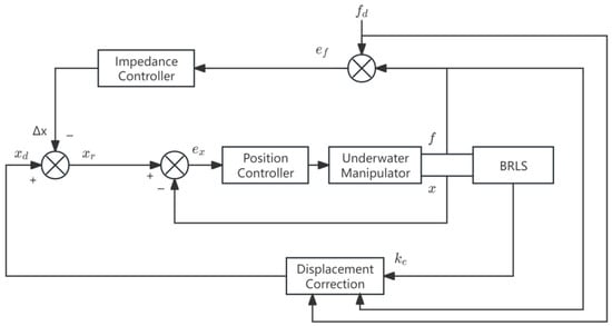
Figure 3. Position-based impedance control block diagram with displacement correction.

4. Fuzzy Adaptive Impedance Control Based on Novel Displacement Correction

Fuzzy control, which exploits fuzzy set theory and fuzzy-logic inference to handle uncertainty and nonlinearity, has demonstrated good engineering applicability and robustness in robotic manipulation, servo drives, and human-robot interaction [39,40]. However, constant-force underwater operations are often carried out in complex environments involving inclined and curved surfaces as well as heterogeneous materials. Under such conditions, system parameters are time-varying and external disturbances are significant, and a fuzzy controller with a single fixed universe of discourse cannot simultaneously suppress force peaks, shorten settling time, and reduce steady-state error. To improve control consistency and robustness under such working conditions, various enhanced schemes, such as variable-universe fuzzy control and adaptive fuzzy-parameter tuning, have been proposed, and their effectiveness in reducing overshoot and improving dynamic performance has been validated in many industrial applications.

4.1. Design of the Fuzzy Adaptive Controller

To exploit the environment stiffness identified online by BRLS for fuzzy adaptive impedance tuning, the estimated stiffness is first passed through a low-pass filter and normalized to construct a dimensionless stiffness-perception variable $\xi \left(\mathrm{k}\right)$, which is defined as:

$$\left\{\begin{array}{l}{\tilde{k}}_e(k)=(1-\beta ){\widehat{k}}_e(k)+\beta {\tilde{k}}_e(k-1)\\ \xi (k)={\mathrm{sat}}_{[0,1]}\left({\displaystyle \frac{{\tilde{k}}_e(k)-k_{\mathrm{soft}}}{k_{\mathrm{hard}}-k_{\mathrm{soft}}}}\right)\end{array}\right.$$

(24)

In this definition, ${\widehat{k}}_e(k)$ denotes the environment-stiffness estimate obtained by the BRLS algorithm, ${\tilde{k}}_e(k)$ denotes its low-pass-filtered value, $\beta \in (0,1)$ is the filtering coefficient, $k_{\mathrm{soft}}$ and $k_{\mathrm{hard}}$ are the reference stiffness values for soft and hard environments, respectively, and ${\mathrm{sat}}_{[0,1]}(\cdot )$ is the saturation operator on the interval [0, 1], ensuring that the stiffness perception $\xi \in [0,1]$, with $\xi =0$ indicating a relatively soft environment and $\xi =1$ indicating a relatively stiff environment.

During the first few contact samples, the stiffness estimate can be biased by small displacement increments and contact transients, which may otherwise lead to overly aggressive or overly conservative impedance scheduling. To prevent such early-frame misperception from propagating directly into force regulation, the estimate is low-pass filtered, normalized, and saturated to form the stiffness-perception variable, and the impedance parameters are further updated under amplitude limitation and first-order filtering. This design confines the influence of early estimation errors to a short transient and avoids persistent degradation of force-tracking performance.

To match the fuzzy linguistic sets and to allow signals with different physical units to be processed within a common universe of discourse, the force error $e_f$, the force-error rate ${\dot{e}}_f$, and the stiffness perception $\xi$ are normalized. The normalized variables are defined as:

$$\left\{\begin{array}{l}{\overline{e}}_f={\displaystyle \frac{e_f}{S_f}}\\ {\overline{\dot{e}}}_f={\displaystyle \frac{{\dot{e}}_f}{S_{\dot{f}}}}\\ \overline{\xi }=2\xi -1\end{array}\right.$$

(25)

where ${\overline{e}}_f$, ${\overline{\dot{e}}}_f$ and $\overline{\xi }$ denote the normalized inputs, with $\overline{\xi }\in$ [−1, 1]; $S_f$ and $S_{\dot{f}}$ are positive scaling factors that map $e_f$ and ${\dot{e}}_f$ into the working range [−1, 1], which is convenient for defining the fuzzy linguistic terms.

A fuzzy adaptive impedance controller with three inputs and two outputs is adopted in this paper. The input variables consist of the force error $e_f$, the rate of change of the force error ${\dot{e}}_f$ and the stiffness perception $\xi$ obtained from online identification, whereas the output variables are the desired damping $b_d$ and the desired stiffness $k_d$. To match the task contact force, system bandwidth, and actuator capability, the nominal operating ranges of the non-normalized variables are specified as $e_f\in$ [−6, 6], ${\dot{e}}_f\in$ [−60, 60], $\xi \in$ [0, 1], ${\mathrm{b}}_d\in$ [10, 40], and ${\mathrm{k}}_d\in$ [200, 450]. These bounds are selected as nominal operating ranges under the simulation conditions in Section 5, so that the normalized inputs in Equation (25) remain within [−1, 1] for typical transients, while the saturation operator handles rare out-of-range peaks. The damping and stiffness bounds are consistent with the amplitude limits enforced in Equation (27), which are set according to the closed-loop bandwidth and conservative safety margins. Both inputs and outputs adopt a seven-level fuzzy linguistic set {NB, NM, NS, ZO, PS, PM, PB} (negative big, negative medium, negative small, zero, positive small, positive medium, positive big). Gaussian membership functions are employed and are evenly distributed over their respective universes of discourse, with approximately 50% overlap between adjacent functions and moderate extension at the boundaries to ensure smooth defuzzification. These universes and membership functions also facilitate subsequent fine-tuning of the centers and widths based on experimental data. The fuzzy tuner adopts a standard rule-based inference procedure: the rule base in Table 1 determines the activation of the output linguistic terms, and the resulting aggregated activations are mapped to continuous impedance parameters via centroid defuzzification.

Table 1. Baseline rule table (baseline linguistic levels based on $e_f$ and ${\dot{e}}_f$; outputs: damping level/stiffness level).

${\mathit{e}}_{\mathit{f}}/{\dot{\mathit{e}}}_{\mathit{f}}$	NB	NM	NS	ZO	PS	PM	PB
NB	NS/PB	NS/PM	ZO/PM	ZO/NM	ZO/NM	PS/NS	PS/NS
NM	NS/PM	ZO/PM	ZO/PM	ZO/NS	PS/NS	PS/NS	PM/ZO
NS	ZO/PM	ZO/PM	PS/PS	PS/NS	PS/ZO	PM/ZO	PM/NS
ZO	ZO/PM	PS/PS	PS/ZO	ZO/ZO	PS/ZO	PM/NS	PM/NS
PS	PS/PM	PS/PS	PM/ZO	PM/ZO	PM/ZO	PM/NS	PB/NS
PM	PS/PM	PM/PS	PM/PS	PM/ZO	PM/NS	PB/NS	PB/ZO
PB	PM/PM	PM/PS	PM/ZO	PM/ZO	PB/NS	PB/ZO	PB/PS

4.2. Construction of the Fuzzy Rule Table

To obtain stable and reasonable parameter settings under fixed universes of discourse and predefined membership functions, a rule table is first constructed according to the force error $e_f$ and its rate of change ${\dot{e}}_f$, thereby determining the baseline linguistic levels of the desired damping and desired stiffness [41]. The design of the rules follows the principles below:

• When $\left|e_f\right|$ is large and ${\dot{e}}_f$ > 0 (the error is increasing), the damping should be increased and the stiffness should be moderately raised in order to suppress transient force peaks and accelerate convergence.
• When $e_f$ < 0 and ${\dot{e}}_f$ < 0 (the error is changing in the opposite direction), strong damping and relatively weak stiffness are selected to reduce overshoot and secondary rebound.
• In the small-error region ($e_f$ ≈ 0, ${\dot{e}}_f$ ≈ 0), both outputs should approach zero or be adjusted only slightly so as to avoid parameter chattering induced by measurement noise.

The rule base is constructed to be consistent with standard impedance-tuning intuition, and the linguistic partitions are kept symmetric to avoid biased scheduling. In addition, the subsequent amplitude limitation and first-order filtering reduce sensitivity to small modifications of individual rules, such that moderate retuning primarily affects transient aggressiveness rather than closed-loop stability. In this study, the rule table is obtained through expert-guided design and empirical refinement in simulation, and no automated optimization is required to reproduce the reported results.

In Table 1, each cell specifies the linguistic variables of the two outputs in the form “damping level/stiffness level”, using the linguistic set {NB, NM, NS, ZO, PS, PM, PB}. The third input (stiffness perception) does not introduce an additional rule dimension; instead, it applies a bounded level bias to the baseline output levels obtained from Table 1, as detailed in Table 2 and Table 3.

Table 2. Scheduling of the desired damping based on the stiffness perception.

$\mathit{\xi }$ Level	Bias on Desired Damping
Low	Decrease by one level
Mid	No adjustment
High	Increase by one level

Table 3. Scheduling of the desired stiffness based on the stiffness perception.

$\mathit{\xi }$ Level	Bias on Desired Stiffness
Low	Increase by one level
Mid	No adjustment
High	Decrease by one level

The rule base is formulated on normalized inputs and outputs, which facilitates reuse across different manipulators and task settings. For a new platform, the primary adaptation typically lies in rescaling the normalization bounds and membership-function widths to match actuator capability and sensing resolution, while the qualitative rule logic remains unchanged. When facing substantially different interaction regimes, the same structure can be extended by introducing task-specific scaling layers rather than expanding the rule table indiscriminately.

While the proposed fuzzy inference provides an interpretable and implementation-friendly tuning mechanism, data-driven alternatives could be used to learn or refine the tuning map under stability-preserving bounds. Exploring such learning-based tuning is beyond the scope of this study and is left for future work.

After obtaining the baseline levels in Table 1, the stiffness perception $\xi$ is further used to bias the desired damping level. In general, a “harder” environment (large $\xi$) requires a higher damping level to suppress contact-force peaks, whereas a “softer” environment (small $\xi$) favors a lower damping level to avoid excessive viscosity. Concretely, a bias of “increase one level/no adjustment/decrease one level” is superimposed on the baseline levels in Table 1, and saturation is applied at the boundaries of the linguistic set {NB, NM, NS, ZO, PS, PM, PB}. The detailed mapping from $\xi$ levels to the corresponding damping offsets is given in Table 2.

Similarly, the desired stiffness is scheduled using the same strategy. In a soft environment, the stiffness is moderately increased to improve force response and positioning rigidity, whereas in a hard environment, the stiffness is moderately reduced to attenuate transient contact-force peaks and overshoot. Concretely, a stiffness bias of “increase one level/no adjustment/decrease one level” is superimposed on the baseline levels in Table 1, and saturation is applied at the boundaries of the linguistic set {NB, NM, NS, ZO, PS, PM, PB}. The detailed mapping from $\xi$ levels to the corresponding stiffness offsets is given in Table 3.

4.3. Defuzzification and Parameter-Update Strategy

Based on the fuzzy rule base and the membership functions, the aggregated activation degrees of all output linguistic terms at the current time instant are first obtained. To convert this distribution into deterministic parameters that can be directly used in the control law, the centroid method of fuzzy sets is adopted for defuzzification, and the corresponding expression is given by:

$$\left\{\begin{array}{l}{b_d}^{*}={\displaystyle \frac{{\displaystyle \sum _{j=1}^7{\mu }_j^{(b)}}{b}_j}{{\displaystyle \sum _{j=1}^7{\mu }_j^{(b)}}}}\\ {k_d}^{*}={\displaystyle \frac{{\displaystyle \sum _{j=1}^7{\mu }_j^{(k)}}{k}_j}{{\displaystyle \sum _{j=1}^7{\mu }_j^{(k)}}}}\end{array}\right.$$

(26)

where ${b_d}^{*}$ and ${k_d}^{*}$ denote the defuzzified desired damping and desired stiffness, respectively; ${\mu }_j^{(b)}$ and ${\mu }_j^{(k)}$ represent the aggregated activation degrees of the j-th output linguistic term over the seven levels from NB to PB; $b_j$ and $k_j$ are the representative values of that linguistic term in the corresponding output universes of discourse. Equation (26) essentially performs a weighted centroid operation over all activated rules: the larger the activation degree, the greater the contribution to the final defuzzified value. Compared with the max-membership method, the centroid method produces smoother outputs and is less sensitive to noise, making it more suitable for online parameter tuning.

Considering actuator capability and closed-loop bandwidth constraints, amplitude limits are imposed on the defuzzified parameters in Equation (26) to avoid unrealizable excitation due to parameter saturation. These amplitude limits also help moderate actuation demand during fast transitions, which is beneficial for power-limited underwater platforms. This yields:

$$\left\{\begin{array}{l}{b}_{\mathrm{tgt}}=\mathrm{sat}(b_d;b_{\min },b_{\max })\\ k_{\mathrm{tgt}}=\mathrm{sat}(k_d;k_{\min },k_{\max })\end{array}\right.$$

(27)

where $b_{\mathrm{tgt}}$ and $k_{\mathrm{tgt}}$ denote the target damping and stiffness after amplitude limiting, and $\mathrm{sat}(\cdot )$ is the saturation function that clips its argument to the bounds $[b_{\min },b_{\max }]$ or $[k_{\min },k_{\max }]$. The limits $b_{\min }$, $b_{\max }$, $k_{\min }$ and $k_{\max }$ are determined by the system bandwidth, actuator capability, and safety margins. Equation (27) thus prevents excessively large desired damping and stiffness, avoiding unrealizable control commands caused by actuator saturation and overly fast inner-loop updates.

To suppress discontinuities and transient oscillations induced by abrupt parameter changes, the target parameters obtained from Equation (27) are further processed by a first-order lag filter in discrete form as:

$$\left\{\begin{array}{l}{b}_d(k)=b_d^{+}(k-1)+{\displaystyle \frac{T_s}{{\tau }_b}}\left(b_{\mathrm{tgt}}-b_d^{+}(k-1)\right)\\ k_d(k)=k_d^{+}(k-1)+{\displaystyle \frac{T_s}{{\tau }_k}}\left(k_{\mathrm{tgt}}-k_d^{+}(k-1)\right)\end{array}\right.$$

(28)

where $b_d(k)$ and $k_d(k)$ denote the final online impedance parameters that are applied to the control law at the k-th sampling instant, $T_s$ is the sampling period, and ${\tau }_b$ > 0 and ${\tau }_k$ > 0 are the time constants for parameter updating, which regulate the tracking speed and smoothness of the adaptation. Consequently, the variables $(e_f,{\dot{e}}_f,\xi )$ are mapped, through the sequence “rule base → defuzzification → amplitude limitation → first-order filtering”, to continuous and realizable impedance parameters $b_d$ and $k_d$.

The transient performance is ultimately limited by the effective bandwidth of sensing, estimation, and inner-loop tracking. When the environment stiffness varies on a time scale comparable to the closed-loop bandwidth, a finite adaptation lag may remain unavoidable, which can manifest as short transient force peaks despite the adopted smoothing and rate limiting.

Accordingly, the filtering bandwidth introduces a practical trade-off between responsiveness and noise rejection. Smaller time constants yield faster parameter adaptation and improved transient responsiveness, but they transmit more measurement noise and may increase high-frequency force ripple. Conversely, larger time constants improve smoothness and robustness to noise at the cost of increased adaptation lag during rapid stiffness variations.

Building on the impedance-control structure with novel displacement correction, a fuzzy adaptive tuning mechanism is further introduced to form the final compliant control system, as illustrated in Figure 4. The fuzzy-logic block serves as a supervisory impedance-parameter tuner for the position-based impedance controller, rather than a standalone controller that directly generates the actuation command. The fuzzy controller adjusts the impedance parameters in real time, so that the damping and stiffness automatically adapt to large variations in both contact force and environment stiffness, thereby achieving coordinated force-displacement regulation. By exploiting the environment-stiffness information provided by the BRLS-based identification module, the system can adaptively modify the control parameters under continuous-contact conditions, maintaining stability and compliance during interaction. This control architecture is particularly suitable for underwater manipulator operations, as it effectively suppresses external disturbances in complex variable-stiffness environments, improves the accuracy of end-effector contact-force regulation, and enhances operational safety.

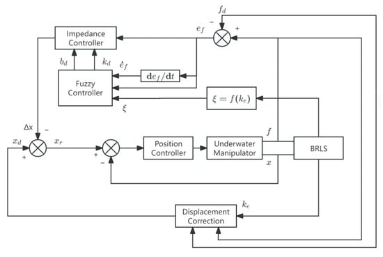
Figure 4. Block diagram of displacement-corrected fuzzy adaptive impedance control.

4.4. Stability and Boundedness Analysis

This stability analysis concerns the outer displacement-compensation dynamics embedded in the position-based impedance-control framework in Figure 4. The inner position-control loop is assumed to be stable and sufficiently fast, such that the residual position-tracking mismatch can be treated as a bounded perturbation in the outer-loop dynamics, consistent with the inner-loop fast-tracking approximation adopted in Equation (30). For clarity, the variables appearing in Equations (29)–(41) are explicitly defined in the text, and the ISS argument follows standard Lyapunov and comparison-lemma results in nonlinear systems theory [42]. Here, the force error is formed by the force reference and the measured contact force, and the disturbance term aggregates the effects of the unmeasured environment position, stiffness-identification error, measurement noise, and bounded inner-loop imperfections.

For convenience of analysis, let the final reference displacement be defined as $x_r=x_d+\Delta x$, and define the force error as $e_f=f-f_d$. The dynamic response of the displacement-compensation subsystem to the force error can be written as:

$$\Delta \ddot{x}+b_d(t)\Delta \dot{x}+k_d(t)\Delta x=-e_f$$

(29)

where $b_d(t)$ > 0 and $k_d(t)$ > 0 denote the final online impedance parameters entering the control law after the “defuzzification → amplitude limitation → first-order filtering” process.

From the contact model $f=k_e(x-x_e)$ and the inner-loop fast-tracking approximation $x\approx x_r=x_d+\Delta x$, this yields:

$$e_f=k_e\Delta x+\left[\begin{array}{c}{k}_e(x_d-x_e)-f_d\end{array}\right]$$

(30)

where $a(t)\in {\mathcal{L}}_{\infty }$ collects the effects of the unmeasured environment position, stiffness-identification error, and measurement noise as a bounded disturbance.

In practice, finite inner-loop bandwidth, actuator backlash, and latency can introduce a nonzero tracking error between the reference and the actual position. From the outer-loop perspective, these imperfections enter the displacement-compensation dynamics as additional bounded perturbations and can be absorbed into the disturbance term. The ISS conclusion therefore remains applicable provided that the inner-loop tracking error is bounded, although degraded inner-loop accuracy may enlarge the ultimate bound and slow the outer-loop transient response.

Substituting Equation (30) into Equation (29) yields the closed-loop equation in terms of $\Delta x$:

$$\Delta \ddot{x}+b_d(t)\Delta \dot{x}+\left(k_d(t)+k_e(t)\right)\Delta x=-\alpha (t)$$

(31)

Assume that there exist positive constants $b_{\min }>0$, $k_{\min }>0$ and ${\overline{k}}_1>0$ such that $b_d(t)\in [b_{\min },b_{\max }]$, $k_d(t)\in [k_{\min },k_{\max }]$, and $|{\dot{k}}_d(t)+{\dot{k}}_e(t)|\le \overline{k}$, and that $\alpha (t)\in {\mathcal{L}}_{\infty }$. Define: $\underset{\_}{k}:={\inf }_t(k_d(t)+k_e(t))>0$.

These boundedness conditions are consistent with practical hardware constraints of underwater manipulators operated under actuator saturation, workspace limitations, and safety-constrained interaction forces. In implementation, the amplitude limitation and first-order filtering mechanisms explicitly keep the scheduled impedance parameters within realizable ranges, while the inner position servo and sensor conditioning are designed to maintain tracking errors and measurement noise within finite envelopes. Under such hardware-imposed limits, the aggregated disturbance term admits a bounded representation, thereby supporting the applicability of the ISS-based stability analysis.

By applying the comparison lemma to the Lyapunov differential inequality obtained from Equation (31), the ISS conclusion follows. Under the above assumptions, system (31) is input-to-state stable (ISS) with respect to the input $a(t)$. Moreover, if $\alpha (t)\to 0$ and $k_d(t)$, ${\dot{k}}_e(t)$ converge asymptotically to constant values, then $\Delta x(t)\to 0$ and $\Delta \dot{x}(t)\to 0$.

Proof: Consider the Lyapunov function:

$$V={\displaystyle \frac{1}{2}}\Delta {\dot{x}}^2+{\displaystyle \frac{1}{2}}\left(k_d(t)+k_e(t)\right)\Delta x^2$$

(32)

Differentiating Equation (31) and rearranging yields:

$$\dot{V}=-b_a(t)\Delta {\dot{x}}^2-\alpha (t)\Delta \dot{x}+{\displaystyle \frac{1}{2}}\left({\dot{k}}_a(t)+{\dot{k}}_e(t)\right)\Delta x^2$$

(33)

By Young’s inequality, for any $\eta >0$, we have:

$$-\alpha \Delta \dot{x}\le {\displaystyle \frac{\eta }{2}}\Delta {\dot{x}}^2+{\displaystyle \frac{1}{2\eta }}{\alpha }^2(t)$$

(34)

Combining Equation (34) with the bound $\left|{\dot{k}}_a(t)+{\dot{k}}_e(t)\right|\le {\overline{k}}_1$ yields:

$$\dot{V}\le -\left(b_a(t)-{\displaystyle \frac{\eta }{2}}\right)\Delta {\dot{x}}^2+{\displaystyle \frac{{\overline{k}}_1}{2}}\Delta x^2+{\displaystyle \frac{1}{2\eta }}{\alpha }^2(t)$$

(35)

Moreover, since:

$$V\ge {\displaystyle \frac{1}{2}}\Delta {\dot{x}}^2+{\displaystyle \frac{1}{2}}{k}_{*}\Delta x^2$$

(36)

we obtain the bounds:

$$\Delta {\dot{x}}^2\le 2V,\hspace{1em}\Delta x^2\le {\displaystyle \frac{2}{k_{*}}}V$$

(37)

Consequently, substituting the bounds in Equations (36) and (37) into the right-hand side of Equation (34) yields:

$$\dot{V}\le -\left(2b_{\min }-\eta -{\displaystyle \frac{{\overline{k}}_1}{k_{*}}}\right)V+{\displaystyle \frac{1}{2\eta }}{\alpha }^2(t)$$

(38)

Let:

$${\beta }_1:=2b_{\min }-\eta -{\displaystyle \frac{{\overline{k}}_1}{k_{*}}}>0,\hspace{1em}{\beta }_3:={\displaystyle \frac{1}{2\eta }}$$

(39)

and choose $\eta \in (0,2b_{\min }-{\displaystyle \frac{{\overline{k}}_1}{k_{*}}})$ so that ${\beta }_1$ > 0. Then Equation (38) can be rewritten as:

$$\dot{V}\le -{\beta }_{1}V+{\beta }_3{\alpha }^2(t)$$

(40)

Accordingly, since Equation (40) is derived in the presence of the bounded disturbance term aggregated in Equation (30), it is not required to be strictly negative for all time. In Equation (40), the coefficient $\eta$ is defined in Equation (39) and is enforced to be strictly positive by an appropriate choice of $\epsilon$. With $\eta$ > 0, the dissipative part in Equation (40) dominates whenever the Lyapunov function is sufficiently large, which guarantees that the solution enters and remains in a bounded neighborhood whose size depends on the disturbance bound. This is the standard input-to-state stability (ISS) interpretation adopted in the analysis.

By the comparison lemma, Equation (40) implies:

$$V(t)\le e^{-{\beta }_{1}t}V(0)+{\displaystyle \frac{{\beta }_3}{{\beta }_1}}\underset{0\le \tau \le t}{\sup }{\alpha }^2(\tau )$$

(41)

Using the equivalence between V and $(\Delta x,\stackrel{.}{\Delta x})$, the closed-loop system is input-to-state stable with respect to $\alpha (t)$. Furthermore, when $\alpha (t)\to 0$ and $k_a(t)$, $k_e(t)$ converge to constant values (equivalently, ${\dot{k}}_a(t),{\dot{k}}_e(t)\to 0$), one has $V(t)\to 0$, i.e., $\Delta x(t)\to 0$ and $\Delta \dot{x}(t)\to 0$.

5. Results

To evaluate the effectiveness of the proposed BRLS-FAIC scheme, MATLAB R 2022a simulations of coordinated force-position control at the end-effector are conducted based on the established underwater manipulator dynamic model and the overall control architecture. For online stiffness identification, three estimators are implemented and compared: recursive least squares (RLS), adaptive-forgetting recursive least squares (AF-RLS), and BRLS. The test conditions cover three representative stiffness profiles (step, linear ramp, and sinusoidal variation) and three typical contact geometries (planar, inclined-plane, and sinusoidal surfaces), thereby emulating a broad range of underwater contact tasks. Classical impedance control (IC) and fuzzy adaptive impedance control (FAIC) are implemented as baselines under an identical inner position-control loop and the same manipulator parameters to ensure a fair and systematic comparison. The main simulation parameters and identification settings are summarized in Table 4.

Table 4. Main simulation parameters.

Parameter	Description	Value
$f_d$	Reference contact force	20 N
$m_d$	Target mass	1 kg
$b_d$	Initial target damping	0.08 N·s/mm
$k_d$	Initial target stiffness	1.2 N/mm
$k_0$	Initial environment stiffness	10 N/mm
$P_0$	Initial covariance	10,000 $I$
Q	Nominal process-noise variance	0.0001
R	Nominal measurement-noise variance	0.001
$\alpha$	Force-error smoothing factor	0.94
${\tau }_b$	Damping update time constant	0.05 s
${\tau }_k$	Stiffness update time constant	0.08 s
$T_s$	Sampling period	0.002 s

All simulations are conducted with a sampling period of 0.002 s. A lower sampling rate reduces the effective bandwidth of sensing and estimation updates and may increase the apparent scheduling latency; accordingly, the smoothing and update time constants should be re-tuned to preserve stability margins and tracking smoothness under low-frequency perception hardware.

Force-tracking performance is evaluated from the contact-force trajectory and force-tracking error, whereas position-tracking performance is evaluated from the end-effector trajectory and position error. In addition, the overshoot and settling time of both force and position responses are extracted from the simulation data, enabling quantitative comparison of transient behavior and steady-state accuracy among the different estimators and control schemes.

In this study, the term “external perturbations” is mainly represented by abrupt or continuous variations of the interaction conditions, rather than by an additional injected disturbance signal. The stiffness step in Figure 5 and Figure 6 constitutes a step-like perturbation at the contact interface, and the linear and sinusoidal stiffness profiles in Figure 7, Figure 8, Figure 9 and Figure 10 represent slowly varying and periodic perturbations, respectively. The contact-surface cases in Figure 11, Figure 12, Figure 13, Figure 14, Figure 15 and Figure 16 further evaluate robustness against geometry-induced coupling disturbances in planar, inclined, and curved contacts.

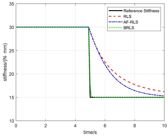
Figure 5. Environment-stiffness identification under a step change.

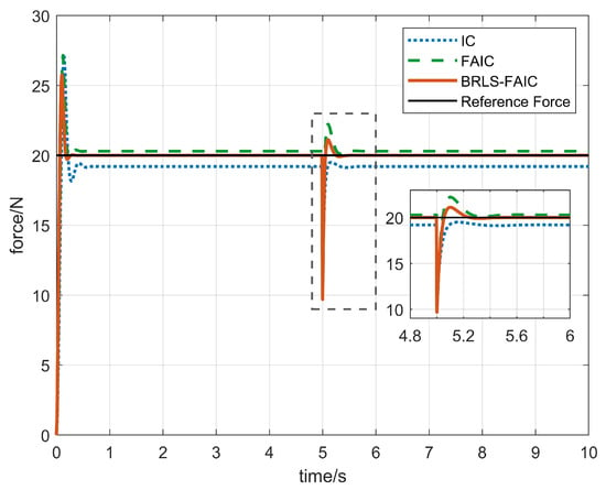
Figure 6. Force-tracking response under a step change in environment stiffness.

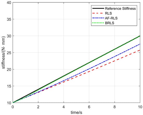
Figure 7. Environment-stiffness identification under a linear variation.

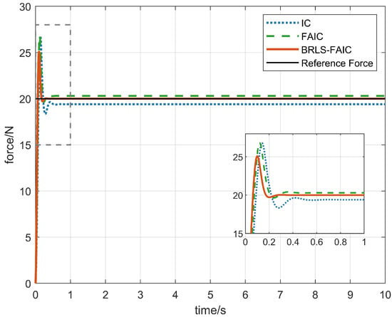
Figure 8. Force-tracking response under a linear variation in environment stiffness.

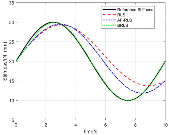
Figure 9. Environment-stiffness identification under sinusoidal stiffness variation.

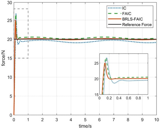
Figure 10. Force-tracking response under a sinusoidal variation in environment stiffness.

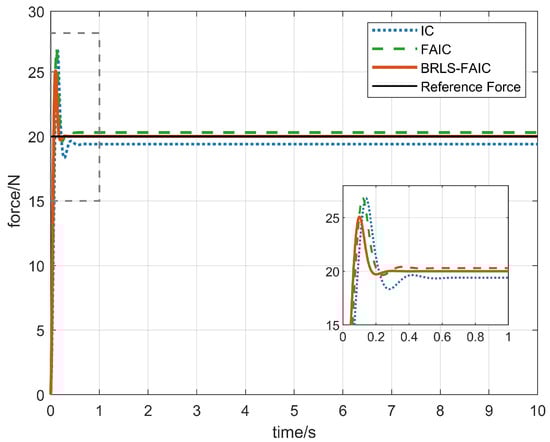
Figure 11. Force-tracking response for planar contact.

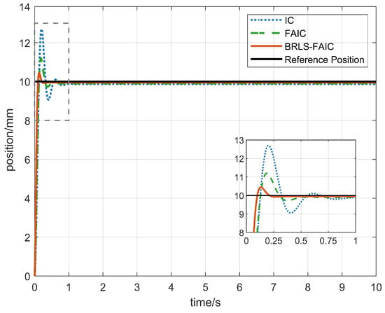
Figure 12. Position-tracking response for planar contact.

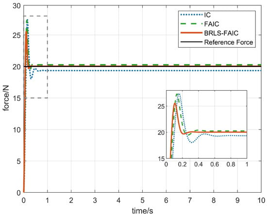
Figure 13. Force-tracking response for inclined-plane contact.

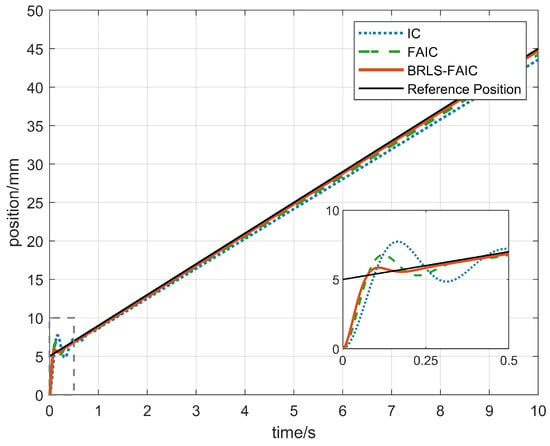
Figure 14. Position-tracking response for inclined-plane contact.

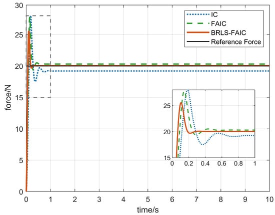
Figure 15. Force-tracking response for curved-surface contact.

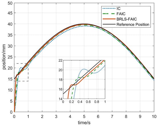
Figure 16. Position-tracking response for curved-surface contact.

5.1. Force Tracking Under a Step Change in Environment Stiffness

Figure 5 compares the reference environment stiffness with the outputs of three online identification methods. The end-effector is in contact with the environment; the stiffness is 30 N/mm for 0–5 s and steps to 15 N/mm at t = 5 s. After the jump, RLS and AF-RLS exhibit a noticeable lag accompanied by overshoot and undershoot, requiring a longer transient to settle to the new stiffness. In contrast, BRLS rapidly approaches the reference after the jump with small overshoot and a short transient, and then almost coincides with the reference curve, indicating better adaptability and robustness to abrupt parameter changes.

Figure 6 shows the corresponding force-tracking responses with a 20 N reference force. All methods display a short initial regulation phase, and all present a momentary undershoot at the stiffness step at t = 5 s. IC yields the largest undershoot, the slowest decay of oscillations, and a nonzero steady-state bias. FAIC reduces the bias to some extent, but post-jump oscillations remain evident. BRLS-FAIC produces a smaller undershoot, shorter and weaker oscillations, and the fastest return to the reference; in the interval 5.0–5.6 s, its recovery speed and stability are clearly superior to those of the two comparative methods.

Taken together, Figure 5 and Figure 6 indicate that, under stiffness jumps, BRLS-FAIC outperforms the comparative methods IC and FAIC in terms of dynamic response, disturbance rejection, and steady-state force-tracking error, and recovers more quickly to maintain a contact force close to the reference.

5.2. Force Tracking Under a Linear Variation of Environment Stiffness

Figure 7 shows the identification results under a linearly varying environment stiffness. The reference stiffness increases linearly from 10 N/mm to 30 N/mm. Throughout the process, RLS exhibits pronounced lag and a negative bias; AF-RLS improves the tracking ability but still maintains a visible gap from the reference. In contrast, BRLS nearly coincides with the reference, exhibiting the smallest overall lag and the most accurate tracking, and thus provides stable online estimates under continuously varying parameters.

Figure 8 presents the corresponding force-tracking responses with a 20 N reference force. All three control schemes show a short initial overshoot and oscillation. IC has a longer settling time and a steady-state force slightly below the reference; FAIC yields a steady-state bias slightly above the reference and more pronounced early oscillations. BRLS-FAIC exhibits smaller overshoot and faster convergence in the magnified interval 0–1 s, and subsequently maintains close adherence to the reference force with small fluctuations as the environment stiffness continues to increase.

Overall, Figure 7 and Figure 8 indicate that, under linearly varying stiffness, BRLS-FAIC outperforms the comparative methods IC and FAIC in terms of dynamic response speed, disturbance suppression, and steady-state force-tracking error, thereby enabling more stable force tracking for underwater manipulator tasks.

5.3. Force Tracking Under a Sinusoidal Variation of Environment Stiffness

Figure 9 reports the identification results under a sinusoidally varying environment stiffness. The reference stiffness oscillates between 10–30 N/mm, with a peak near t ≈ 3 s and a trough near t ≈ 7 s. RLS exhibits pronounced phase lag and amplitude bias throughout, with insufficient tracking on both the rising and falling segments; AF-RLS reduces the lag but still shows visible gaps around the peaks and valleys. In contrast, BRLS closely follows the reference, aligning well with both peak/trough locations and amplitudes, and tracks promptly on both the up- and down-slopes.

Figure 10 presents the corresponding force-tracking responses with a 20 N reference force. All methods show a brief initial overshoot and oscillation. As the stiffness varies periodically, IC falls below the reference for most intervals and exhibits more pronounced oscillations, while FAIC exceeds the reference in some intervals with larger fluctuations. BRLS-FAIC exhibits smaller overshoot and faster convergence in the magnified 0–1 s window and, once in steady operation, provides stronger suppression of periodic disturbances; the contact force remains close to the reference with smaller amplitude variations.

Overall, Figure 9 and Figure 10 show that periodic stiffness variation imposes persistent disturbances on the contact force. BRLS-FAIC maintains small phase lag and amplitude bias over the entire cycle, with a narrow-band force trajectory around the reference and no evident drift or secondary oscillations, demonstrating superior adaptability to continuously varying parameters. This makes it more suitable for stable force tracking and long-duration operation of underwater manipulators on undulating surfaces.

5.4. Force Tracking on a Planar Contact Surface

Figure 11 presents the force-tracking response in a planar-contact task with a 20 N reference force. All methods exhibit a brief initial regulation phase. IC shows a pronounced overshoot on the rising edge with a long decay of oscillations, and its steady-state force remains slightly below the reference. FAIC reduces the initial overshoot but still exhibits several rebounds before settling. BRLS-FAIC approaches the reference more rapidly during the rise, with a smaller overshoot; once in steady operation, the force fluctuates within a narrower band and remains closely centered around the reference.

Figure 12 shows the corresponding end-effector position-tracking performance. IC produces a visible step overshoot followed by a slow return; FAIC lowers the overshoot but retains a nonzero steady-state error. BRLS-FAIC achieves a shorter rise time with better overshoot suppression; the position error converges within a shorter interval and then remains with small-amplitude variations, without secondary oscillations.

Overall, Figure 11 and Figure 12 indicate that, in planar contact, BRLS-FAIC provides more robust force-position coordination for underwater manipulators. Compared with the comparative methods IC and FAIC, it generates a force trajectory closer to the reference and a faster convergence of the position error, making it suitable for planar tasks that require both high steady-state accuracy and short settling time.

5.5. Force Tracking on an Inclined Plane

Figure 13 shows the force-tracking response in an inclined-plane contact task with a 20 N reference force. Due to geometric coupling on the slope, all methods exhibit initial overshoot and oscillation. IC presents a larger undershoot and slower decay, with a steady-state force below the reference. FAIC reduces the initial fluctuation but still shows multiple rebounds before settling. BRLS-FAIC approaches the reference more rapidly, with smaller overshoot and a shorter oscillation duration, and then oscillates within a narrow band around the reference in steady operation.

Figure 14 reports the corresponding position-tracking results. IC produces a pronounced overshoot on the rising edge and a slow return, leaving a steady-state bias; FAIC lowers the overshoot but, under slope-induced coupling, exhibits slower convergence of the position error. BRLS-FAIC achieves a shorter rise time with better overshoot suppression; the position error converges more quickly and maintains small-amplitude variations without secondary oscillations.

Overall, Figure 13 and Figure 14 indicate that, in inclined-plane contact, BRLS-FAIC outperforms the comparative methods IC and FAIC in terms of dynamic response, disturbance attenuation, and steady-state accuracy, thereby enabling more reliable force-position coordinated tracking for underwater manipulators.

5.6. Force Tracking on a Curved Surface

Figure 15 presents the force-tracking response in a curved-surface contact task with a 20 N reference force. Owing to continuously varying curvature and contact geometry, all methods exhibit adjustment transients at the outset. IC shows large overshoot and rebounds across multiple segments with a noticeable steady-state bias; FAIC reduces overshoot in some intervals but still exhibits considerable fluctuations and moderate convergence speed. BRLS-FAIC yields smaller undershoot at each transition, shorter oscillation duration, and a narrow-band force trajectory around the reference, recovering quickly as the surface geometry switches.

Figure 16 reports the corresponding position-tracking results. IC produces visible overshoot and slow return at curvature changes, with a relatively large steady-state error; FAIC alleviates overshoot but still develops secondary oscillations after multiple curvature changes. BRLS-FAIC provides smoother rise and decay, superior overshoot suppression, and faster convergence of the position error with smaller residual fluctuations.

Overall, Figure 15 and Figure 16 indicate that, under continuously varying contact geometry on curved surfaces, BRLS-FAIC delivers more stable force-position coordinated tracking for underwater manipulators. It maintains smaller force-tracking and position-tracking errors under repeated geometric changes and parameter disturbances than the comparative methods IC and FAIC, making it suitable for tasks involving undulating surfaces.

It is also noted that extreme geometry changes, such as sharp curvature transitions or near-discontinuous contact normals, can induce rapid variations in the effective contact direction and perceived stiffness. Under such conditions, larger transient force peaks and increased adaptation lag may occur, since the controller must reconcile abrupt geometric changes with finite sensing and update bandwidth. In practice, adopting a more compliant approach impedance and conservative filter bandwidth during expected sharp transitions can improve robustness without altering the proposed control structure.

6. Discussion

The simulation environment and controller settings follow the core parameters listed in Table 4, ensuring that all three methods are evaluated under identical conditions in terms of the reference contact force and the target impedance parameters (mass, damping, and stiffness), thereby guaranteeing comparability and reproducibility.

Under varying-stiffness conditions, Table 5 summarizes the force-tracking performance of the three methods under different stiffness variation cases (step, linear, and sinusoidal). BRLS-FAIC consistently achieves smaller steady-state errors and lower peak contact forces, and exhibits a markedly shorter settling time than the comparative methods IC and FAIC, indicating stronger adaptability and robustness to time-varying stiffness as a result of the BRLS-based stiffness identification and displacement correction.

Table 5. Comparison of force-tracking performance metrics under varying stiffness.

Scenario	Control Method	Steady-State Error (N)	Settling Time (s)	Maximum Overshoot (%)	Peak Contact Force (N)
Step stiffness change	IC	0.82	0.35	36	27.2
	FAIC	0.31	0.19	36	27.1
	BRLS-FAIC	0.01	0.15	29	25.8
Linear stiffness	IC	0.61	0.34	34	26.9
	FAIC	0.32	0.18	34	26.8
	BRLS-FAIC	0.01	0.15	25	25.1
Sinusoidal stiffness	IC	0.62	0.36	33	26.7
	FAIC	0.30	0.21	33	26.6
	BRLS-FAIC	0.01	0.16	25	25.0

While the simulations consider representative stiffness-variation profiles, practical underwater contact may also involve impulsive events such as abrupt shocks or hard collisions. In such cases, the interaction force can exhibit a short spike that is not fully captured by a quasi-static stiffness description, and a transient mismatch may arise before the filtered stiffness perception and impedance scheduling settle. The adopted amplitude limitation, first-order parameter filtering, and smoothed displacement correction provide protective layers that bound the commanded motion and attenuate collision-induced rebounds, thereby improving operational robustness under occasional unmodeled impacts.

Across different contact surfaces, Table 6 and Table 7 summarize the force and position tracking performance of the three methods in planar, inclined-plane, and curved-surface tasks. On all surfaces, BRLS-FAIC maintains smaller steady-state force and position errors and lower overshoot than IC and FAIC, yielding smoother and more stable contact processes. Taken together, Table 5, Table 6 and Table 7 indicate that BRLS-FAIC outperforms the comparative methods in response speed, disturbance attenuation, and tracking accuracy, providing effective support for constant-force operations of underwater manipulators in complex contact environments.

Table 6. Comparison of force-tracking performance metrics across different contact surfaces.

Scenario	Control Method	Steady-State Error (N)	Settling Time (s)	Maximum Overshoot (%)	Peak Contact Force (N)
Planar surface	IC	0.62	0.35	34	26.8
	FAIC	0.32	0.19	34	26.7
	BRLS-FAIC	0.01	0.15	25	25.1
Inclined surface	IC	0.65	0.39	37	27.4
	FAIC	0.26	0.21	37	27.2
	BRLS-FAIC	0.03	0.17	28	25.5
Curved surface	IC	0.82	0.47	40	28.0
	FAIC	0.33	0.23	39	27.7
	BRLS-FAIC	0.03	0.17	28	25.5

Table 7. Comparison of position-tracking performance metrics across different contact surfaces.

Scenario	Control Method	Steady-State Error (mm)	Settling Time (s)	Maximum Overshoot(%)	Maximum Position Error (mm)
Planar surface	IC	0.13	0.65	27	2.70
	FAIC	0.10	0.29	12	1.20
	BRLS-FAIC	0.02	0.18	5	0.45
Inclined surface	IC	1.27	0.37	42	2.11
	FAIC	0.82	0.16	25	1.24
	BRLS-FAIC	0.06	0.06	8	0.42
Curved surface	IC	1.41	0.83	9	1.28
	FAIC	0.82	0.37	4	0.56
	BRLS-FAIC	0.11	0.14	2	0.23

7. Conclusions

This study proposes BRLS-FAIC, an integrated compliance-control strategy that combines displacement correction with FAIC for underwater manipulator contact tasks. The principal novelty of this work is a unified BRLS-FAIC architecture that integrates BRLS-based stiffness identification, stiffness-aware displacement correction, and fuzzy impedance tuning into a single position-based impedance framework, thereby jointly addressing time-varying stiffness, contact-location uncertainty, and realizable online impedance scheduling in underwater contact tasks. Built upon RLS, a BRLS estimator is developed for online identification of environment stiffness, providing reliable real-time information for impedance tuning and displacement correction under complex time-varying contact conditions. The stiffness-aware displacement correction reduces steady-state bias, while the fuzzy adaptation adjusts damping and stiffness online to suppress overshoot, attenuate oscillations, and improve tracking smoothness. Simulation results under step, linear, and sinusoidal stiffness variations and across planar, inclined-plane, and curved-surface contacts show that BRLS-FAIC rapidly attenuates disturbances, reduces force and position errors, and maintains stable outputs, outperforming IC and FAIC and offering a feasible and robust control solution for underwater manipulators in complex dynamic environments.

For practical deployment, the scheduled impedance parameters should remain within realizable bounds consistent with actuator capability and contact safety. In this study, the damping and stiffness were constrained to 0.04–0.12 N·s/mm and 0.6–1.8 N/mm, respectively, for the considered setup, and bounded scheduling with moderate update time constants is advised to avoid excessive inner-loop demands during abrupt contact events. In this context, for higher-DOF systems or heavier end-effectors, the same outer-loop structure can be implemented in task space, while the impedance bounds and inner-loop bandwidth should be re-tuned to accommodate increased inertia and actuator limits. Along these lines, reinforcement learning policy-learning controllers, such as DDPG and TD3, represent an alternative paradigm that may be explored to complement model-based and rule-based tuning in underwater contact regulation. Finally, despite the above benefits, real-world deployment may still be challenged by extremely noisy force sensing, strong unmodeled hydrodynamic disturbances, and pronounced contact nonlinearities; addressing these factors through improved sensing and disturbance handling, together with nonlinear contact modeling, remains an important direction for future work.

References

- Liu, J.; Song, Z.; Lu, Y.; Yang, H.; Chen, X.; Duo, Y.; Chen, B.; Kong, S.; Shao, Z.; Gong, Z.; et al. An Underwater Robotic System with a Soft Continuum Manipulator for Autonomous Aquatic Grasping. IEEE/ASME Trans. Mechatron. 2024, 29, 1007–1018. [Google Scholar] [CrossRef]
- Mazzeo, A.; Aguzzi, J.; Calisti, M.; Canese, S.; Vecchi, F.; Stefanni, S.; Controzzi, M. Marine Robotics for Deep-Sea Specimen Collection: A Systematic Review of Underwater Grippers. Sensors 2022, 22, 648. [Google Scholar] [CrossRef]
- Hachicha, S.; Zaoui, C.; Dallagi, H.; Nejim, S.; Maalej, A. Innovative Design of an Underwater Cleaning Robot with a Two Arm Manipulator for Hull Cleaning. Ocean Eng. 2019, 181, 303–313. [Google Scholar] [CrossRef]
- Wang, Y.; Han, L.; Wang, L.; Zhao, G. Manipulator Oriented Grasp Control Based on Image Recognition. In Proceedings of the 2021 4th International Conference on Electron Device and Mechanical Engineering (ICEDME), Guangzhou, China, 19–21 March 2021; IEEE: Piscataway, NJ, USA, 2021; pp. 205–210. [Google Scholar] [CrossRef]
- Huo, Y.; Gang, S.; Guan, C. FCIHMRT: Feature Cross-Layer Interaction Hybrid Method Based on Res2Net and Transformer for Remote Sensing Scene Classification. Electronics 2023, 12, 4362. [Google Scholar] [CrossRef]
- Shang, D.; Li, X.; Yin, M.; Zhou, S. Dynamic modeling and rotation control for flexible single-link underwater manipulator considering flowing water environment based on modified Morison equation. Ocean Eng. 2024, 291, 116427. [Google Scholar] [CrossRef]
- Ji, W.; Zhang, J.; Xu, B.; Tang, C.; Zhao, D. Grasping mode analysis and adaptive impedance control for apple harvesting robotic grippers. Comput. Electron. Agric. 2021, 186, 106210. [Google Scholar] [CrossRef]
- Cao, H.; He, Y.; Chen, X.; Zhao, X. Smooth adaptive hybrid impedance control for robotic contact force tracking in dynamic environments. Ind. Robot 2020, 47, 231–242. [Google Scholar] [CrossRef]
- Wang, Y.; Jiang, Y.; Jiang, J.; Zhang, H.; Tan, H.; Peng, W.; Wu, H.; Zeng, K. Key technologies of robot perception and control and its intelligent manufacturing applications. Acta Autom. Sin. 2023, 49, 494–513. [Google Scholar] [CrossRef]
- Chen, P.; Zhao, H.; Yan, X.; Ding, H. Force control polishing device based on fuzzy adaptive impedance control. In Intelligent Robotics and Applications; Yu, H., Liu, J., Liu, L., Ju, Z., Liu, Y., Zhou, D., Eds.; Lecture Notes in Computer Science; Springer: Cham, Switzerland, 2019; Volume 11743. [Google Scholar] [CrossRef]
- Xu, J.; Huang, K.; Zhang, T.; Zhao, M.; Ji, A.; Li, Y. Mirror adaptive impedance control of multi-mode soft exoskeleton with reinforcement learning. IEEE Trans. Autom. Sci. Eng. 2025, 22, 6773–6785. [Google Scholar] [CrossRef]
- Gong, D.; Song, Y.; Zhu, M.; Teng, Y.; Jiang, J.; Zhang, S. Adaptive variable-damping impedance control for unknown interaction environment. Mathematics 2023, 11, 4961. [Google Scholar] [CrossRef]
- Hu, J.; Zhuang, Y.; Meng, Q.; Yu, H. Active training control method for rehabilitation robot based on fuzzy adaptive impedance adjustment. Machines 2023, 11, 565. [Google Scholar] [CrossRef]
- Hu, P.; Zhang, L.; Yang, H.; Yang, Y. Model predictive-based compliance control for knee arthroplasty surgical robots. Chin. J. Eng. 2024, 46, 1638–1646. [Google Scholar] [CrossRef]
- Duan, J.; Gan, Y.; Chen, M.; Dai, X. Adaptive variable impedance control for dynamic contact force tracking in uncertain environment. Robot. Auton. Syst. 2018, 102, 54–65. [Google Scholar] [CrossRef]
- Cho, J.; Choi, D.; Park, J.H. Sensorless variable admittance control for human–robot interaction of a dual-arm social robot. IEEE Access 2023, 11, 69366–69377. [Google Scholar] [CrossRef]
- Rhee, I.; Kang, G.; Moon, S.J.; Choi, Y.S.; Choi, H.R. Hybrid impedance and admittance control of robot manipulator with unknown environment. Intell. Serv. Robot. 2023, 16, 49–60. [Google Scholar] [CrossRef]
- Duan, R.; Wang, C.; Chen, C.-Y.; Yang, G.; Chen, L. Variable admittance control by measuring arm impedance. In Intelligent Robotics and Applications, ICIRA 2021; Liu, X., Nie, Z., Yu, J., Xie, F., Song, R., Eds.; Lecture Notes in Computer Science; Springer: Cham, Switzerland, 2021; Volume 13014, pp. 555–567. [Google Scholar] [CrossRef]
- Peng, G.; Chen, C.L.P.; Yang, C. Robust admittance control of optimized robot–environment interaction using reference adaptation. IEEE Trans. Neural Netw. Learn. Syst. 2023, 34, 5804–5815. [Google Scholar] [CrossRef]
- Gu, L.; Huang, Q. Adaptive impedance control for force tracking in manipulators based on fractional-order PID. Appl. Sci. 2023, 13, 10267. [Google Scholar] [CrossRef]
- Zheng, G.; Lei, J.; Hu, L.; Zhang, L. Fuzzy adaptive sliding mode impedance control of fracture reduction robot. IEEE Access 2021, 9, 113653–113665. [Google Scholar] [CrossRef]
- Khan, H.; Abbasi, S.J.; Salman, M.; Lee, M.C. Super twisting sliding mode control-based impedance control for robot arm end-effector force tracking. In Proceedings of the 61st Annual Conference of the Society of Instrument and Control Engineers (SICE), Kumamoto, Japan, 6–9 September 2022; pp. 158–162. [Google Scholar] [CrossRef]
- Fu, J.; Burzo, I.; Ovene, E.; Zhao, J.; Ferrigno, G.; De Momi, E. Optimization-based variable impedance control of robotic manipulator for medical contact tasks. IEEE Trans. Instrum. Meas. 2024, 73, 4004608. [Google Scholar] [CrossRef]
- Zhang, J.; Li, H.; Liu, Q.; Li, S. The model reference adaptive impedance control for underwater manipulator compliant operation. Trans. Inst. Meas. Control 2023, 45, 2135–2148. [Google Scholar] [CrossRef]
- Zhang, J.; Han, P.; Liu, Q.; Yang, J.; Li, S. The adaptive impedance control with desired force fuzzy adjustment for underwater manipulator-compliant operation. Trans. Inst. Meas. Control 2024, 47, 158–169. [Google Scholar] [CrossRef]
- Lu, L.; Liu, Q.; Liang, C.; Tang, X.; Xu, D.; Yang, X.; Han, B. Impedance control for underwater gripper compliant grasping in unstructured environment. In Intelligent Robotics and Applications, ICIRA 2021; Liu, X.J., Nie, Z., Yu, J., Xie, F., Song, R., Eds.; Lecture Notes in Computer Science; Springer: Cham, Switzerland, 2021; Volume 13016, pp. 281–292. [Google Scholar] [CrossRef]
- Yu, D.; Zang, X.; Liu, H. Robust constant contact force control for underwater robot: A sliding mode impedance control approach. In Proceedings of the 4th International Conference on Robotics, Artificial Intelligence and Intelligent Control (RAIIC), Chengdu, China, 4–6 July 2025; pp. 321–325. [Google Scholar] [CrossRef]
- Dai, P.; Lu, W.; Le, K.; Liu, D. Sliding mode impedance control for contact intervention of an 1-AWV: Simulation and experimental validation. Ocean Eng. 2020, 196, 106855. [Google Scholar] [CrossRef]
- Hazem, Z.B.; Saidi, F.; Guler, N.; Altaif, A.H. A Hybrid Reinforcement Learning Framework Combining TD3 and PID Control for Robust Trajectory Tracking of a 5-DOF Robotic Arm. Automation 2025, 6, 56. [Google Scholar] [CrossRef]
- Li, G.; Yu, J.; Chen, X. Adaptive fuzzy neural network command filtered impedance control of constrained robotic manipulators with disturbance observer. IEEE Trans. Neural Netw. Learn. Syst. 2023, 34, 5171–5180. [Google Scholar] [CrossRef]
- Guo, Y.; Peng, J.; Ding, S.; Liang, J.; Wang, Y. Fuzzy-based variable impedance control of uncertain robot manipulator in the flexible environment: A nonlinear force contact model-based approach. J. Intell. Fuzzy Syst. 2023, 45, 10227–10241. [Google Scholar] [CrossRef]
- Zhang, J.; Li, H.; Liu, Z.; Wu, Z.; Yang, J. The nonlinear model reference adaptive impedance control for underwater manipulator operation objects in bilateral teleoperation system. Meas. Control 2024, 57, 1194–1210. [Google Scholar] [CrossRef]
- Barbalata, C.; Dunnigan, M.W.; Petillot, Y. Position/force operational space control for underwater manipulation. Robot. Auton. Syst. 2018, 100, 150–159. [Google Scholar] [CrossRef]
- Shen, Y.; Lu, Y.; Zhuang, C. A fuzzy-based impedance control for force tracking in unknown environment. J. Mech. Sci. Technol. 2022, 36, 5231–5242. [Google Scholar] [CrossRef]
- Xu, L.; Su, T.; Zhang, Z.; Zhang, J.; Liu, S.; Zhao, Q.; Yuan, J.; Huang, C.; Zhao, L.; He, G. An adaptive time-varying impedance controller for manipulators. Front. Neurorobot. 2022, 16, 789842. [Google Scholar] [CrossRef]
- Zhou, B.; Song, F.; Liu, Y.; Fang, F.; Gan, Y. Robust sliding mode impedance control of manipulators for complex force-controlled operations. Nonlinear Dyn. 2023, 111, 22267–22281. [Google Scholar] [CrossRef]
- Shao, H.; Hu, W.; Yang, L.; Wang, W.; Suzuki, S.; Gao, Z. Intelligent Impedance Strategy for Force–Motion Control of Robotic Manipulators in Unknown Environments via Expert-Guided Deep Reinforcement Learning. Processes 2025, 13, 2526. [Google Scholar] [CrossRef]
- Lai, B.; Bernstein, D.S. Generalized forgetting recursive least squares: Stability and robustness guarantees. IEEE Trans. Autom. Control 2024, 69, 7646–7661. [Google Scholar] [CrossRef]
- Li, M.; Zhang, Q. Adaptive robust fuzzy impedance control of an electro-hydraulic actuator. Appl. Sci. 2022, 12, 9575. [Google Scholar] [CrossRef]
- Arefinia, E.; Talebi, H.A.; Doustmohammadi, A. A robust adaptive model reference impedance control of a robotic manipulator with actuator saturation. IEEE Trans. Syst. Man Cybern. Syst. 2020, 50, 409–420. [Google Scholar] [CrossRef]
- Li, Z.; Huang, H.; Song, X.; Xu, W.; Li, B. A fuzzy adaptive admittance controller for force tracking in an uncertain contact environment. IET Control Theory Appl. 2021, 15, 2158–2170. [Google Scholar] [CrossRef]
- Park, J.; Choi, Y. Input-to-State Stability of Variable Impedance Control for Robotic Manipulator. Appl. Sci. 2020, 10, 1271. [Google Scholar] [CrossRef]
Disclaimer/Publisher’s Note: The statements, opinions and data contained in all publications are solely those of the individual author(s) and contributor(s) and not of MDPI and/or the editor(s). MDPI and/or the editor(s) disclaim responsibility for any injury to people or property resulting from any ideas, methods, instructions or products referred to in the content. |
© 2025 by the authors. Licensee MDPI, Basel, Switzerland. This article is an open access article distributed under the terms and conditions of the Creative Commons Attribution (CC BY) license.