Abstract
For modern machines, factories and electric and autonomous vehicles, the importance of vreliable electrical connectors cannot be overstated. With an increasing number of connectors being used in machines, factories and vehicles, ensuring their reliability is crucial for comfort and safety alike. One of the key indicators of reliability is the lifetime of connectors. To evaluate the lifetime of electrical connectors, a testing method and a model for calculating their lifetime based on the test data were developed. The results from these tests were compared to failure analysis data from long-term field operations. The findings indicate that the laboratory tests can accurately reproduce the main failures observed in the field. However, such lifetime tests can be time- and labor-intensive. To address this challenge, a data-driven method is proposed that predicts the lifetime of electrical connectors using statistical analysis of electrical contact resistance data collected from short-term tests. The predictions from this method were compared to actual results obtained from long-term tests. A strong correlation was observed between the contact resistance development in short-term tests and the number of failures in later stages of testing. Thus, apart from predicting the lifetime of connectors, this method can also be applied for failure prognosis in real-time operations.
1. Introduction
1.1. General Introduction
Electrical connectors are widely used in electrical and autonomous systems for conducting electric current and signals across them. The electrical connectors therefore form a vital part of a given system, and their performance and reliability have a direct bearing on the system’s reliability. The failure of the connector to transmit the intended current and/or signal could lead to malfunctioning of the system or subsystem in which it is installed. Depending on the function of the system, the effects of such failures can be wide-ranging and can prove to be catastrophic from a comfort and safety point of view or costly from a service point of view. Due to these factors, determining the reliability of electrical connectors before installing them in the system becomes very important. Considering the relation between installed connectors and the components of a system, the reliability of the connectors is increasingly becoming a significant part of the complete system’s reliability [1].
The quality and reliability of electrical connectors have largely improved in recent decades. But an analysis of end-of-life vehicles still reveals a very small but not neglectable number of connectors in critical states [2]. With an increasing number of connectors being used in vehicles, ensuring their reliability is crucial for comfort and safety alike.
1.2. Loads, Operating Parameters of Connectors and Failure Mechanisms
The determination of the reliability of electrical connectors is a challenging task, arising due to the complex failure mechanisms and high degree of variability in their observed lifetimes [3,4]. Ref. [5] identified different failure mechanisms of electrical connectors, such as silver migration, tin whiskers, different types of corrosion, arc formation, creep failure, different kinds of wear, as well as frictional polymerization. The failure could be a result of a single failure mode or the combination of multiple failure modes acting in the connector system. The different failure modes cause different degrees of degradation in the connector system. The sequence of occurrence of the failure modes is also not clearly distinguishable. The occurrence of stress relaxation causing the reduction in the contact force and the degradation of the contact zone in the form of wear and corrosion are the main indicators of the contact degradation in connectors [2,6]. Even in the idle states, along with the stress relaxation, the temperature fluctuations in the surroundings cause the expansion and contraction of the connector materials, leading to relative motion in the contact zone. The reduction in the contact force affects the effective contact area and hence the contact resistance and joule heating [7]. The increases in the contact resistance and joule heating lead to further changes in the effective contact area through contact spot melting and the formation of new contact spots. The presence of atmospheric elements, like oxygen and organic and inorganic compounds such as polymers and sulfide, in the vicinity of the connector leads to chemical degradation of the contact zone through the formation of highly resistive films on the contact surface. These films reduce the electrically effective conductive area and lead to further increases in the electrical contact resistance and joule heating. The reduced contact force as a result of stress relaxation further inhibits the ability to pierce foreign films and therefore the formation of metallic conducting spots. The change in the contact force, contact resistance and joule heating is a continuous process.
The failure modes acting in the connector system are mainly influenced by the nobility of the coating material. In noble coating materials such as gold and silver, the fretting wear occurs initially, which leads to the gradual wear-off of the protective coating. The electrical contact resistance is limited to the presence of the coating material in the contact zone. Once the underlying base material like copper is exposed to the surrounding environment as a result of the wear-off of the noble coating, the oxidation corrosion sets in, leading to an increase in the contact resistance and failure. In the case of non-noble protective coatings such as tin, the fretting wear and oxidation corrosion are effective from the very beginning. In such cases, the failure could even occur before the wear-off of the protective coating material [2,8].
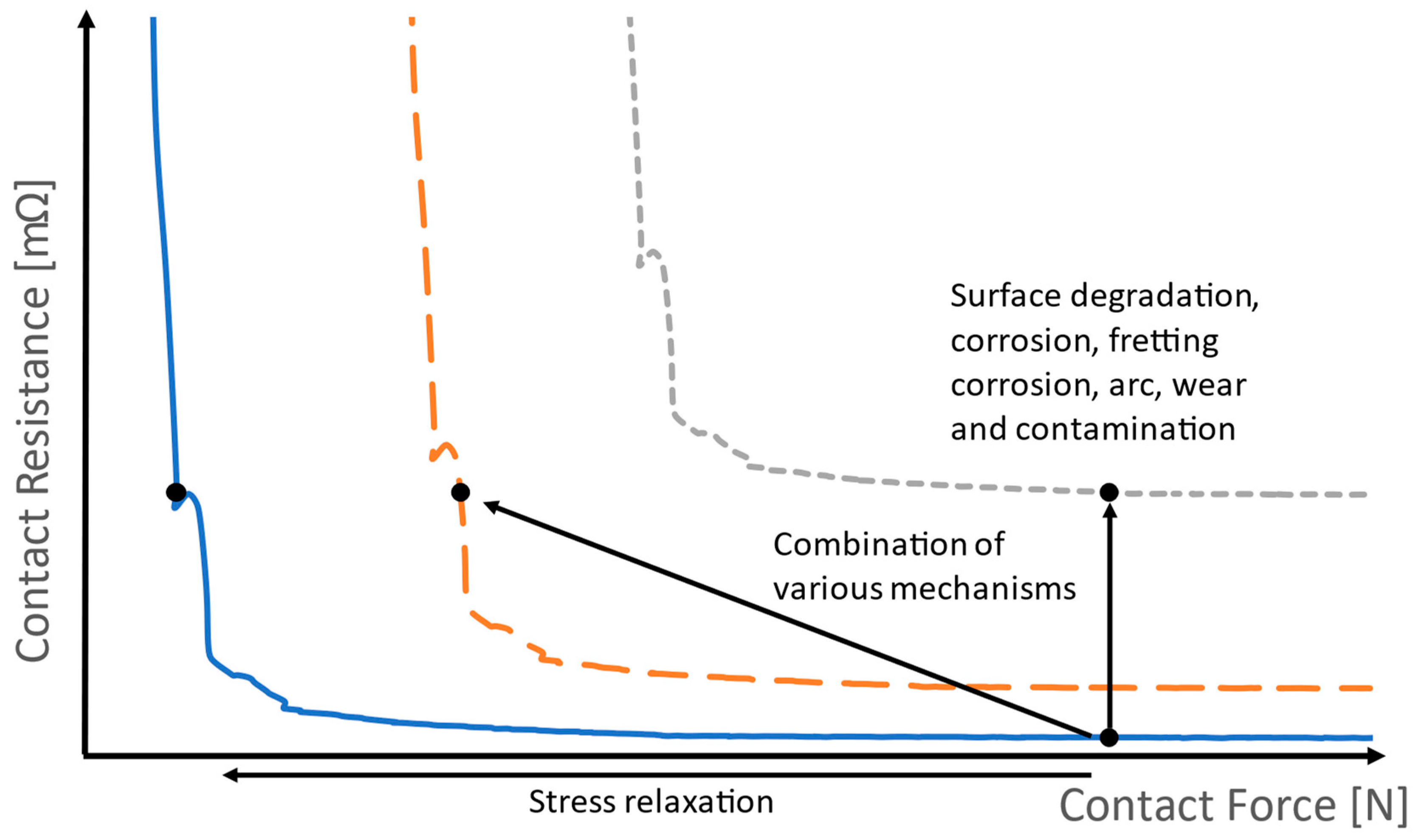
All these mechanisms can lead to a shift in the force–resistance curve, as seen in Figure 1. In most cases, there is a complex combination of several failure mechanisms depending on the respective operation parameters. The operating parameters leading to these failures are resultant of design and environmental factors such as the input current, potential, vibration, contact force, contact geometry, coating thickness, thermal loads, lubrication, humidity, contamination, differential pressure, presence of third bodies in the contact zone, arrangement of contacts, amplitude, direction of relative motion, road conditions, etc.
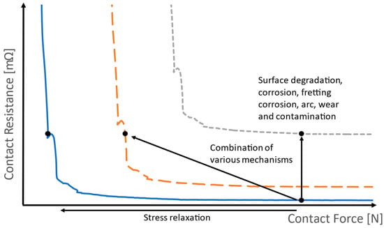
Figure 1.
Schematic illustration of the effect of different failure mechanisms on the force–resistance curves.
2. Reliability Requirements and Accelerated Lifetime Testing
One of the key indicators of reliability is the lifetime of connectors. In order to evaluate the lifetime of electrical connectors, a testing method and a model for the calculation of lifetime based on the test data were developed.
For vehicle applications, only some of the failure mechanisms are relevant. According to an existing study [2], the main causes of failures are fretting of the contact surface, which results in fretting corrosion, and the wear-through of the coating material in combination with oxidation, as well as the stress relaxation resulting from the high operating temperatures. Therefore, it is important to comprehend the influence of vibrational and thermal loads on the connectors, which cause micromotions and wear of the contact surface and eventually lead to the connector failing.
In general, the lifetime or the reliability of a component can be predicted using either a physical-model-based approach, data-driven approach or hybrid approach combining the physical-model-based and data-driven approaches [9,10]. The physical-model-based approach demands in-depth knowledge of the physics of failure to develop a mathematical function defining the relationship between the lifetime-defining performance parameter and the stresses acting on the component. The complex physics of failure in the electrical connector system limits the possibility of the development of a generalized mathematical model for reliability estimation. The data-driven approach can be used for reliability prognosis through the application of the historical performance data of the component. The data-driven model eliminates the need for an in-depth understanding of the system physics of failure, thereby enabling the comparatively easier prognosis of reliability estimation [11,12]. To increase the accuracy of a prognosis through data-driven models, the historical performance data should represent the healthy as well as degraded performance states of the component, i.e., the data recorded should be such that the degradation development from the normal functioning to the failure is recorded. The historical performance data can then be used to train the statistical models or machine learning algorithms to predict the degradation and lifetime. However, there can be challenges in the data collection depending on the time to failure for the corresponding component. Some components have relatively shorter lifetimes and therefore undergo faster degradation. Hence, the data collection of the states representing the healthy and failed conditions is relatively easy compared with components that have very long times to failure and undergo degradation at a slower pace. In the case of electrical connectors, the lifetime could be very long, thereby making the data collection under normal operating stresses almost impractical at times. In the hybrid approach, the physics of failure and the effects of the failure modes are identified, and the corresponding performance parameter is monitored. The data thus collected are then used for training using the data-driven approach to predict the lifetime and reliability. In the field of reliability estimations of electrical connectors, the majority of the investigations for prognosis of reliability and lifetime are either based on data-driven models [13,14,15] or a combination of physical and data-driven models [9,16,17].
Therefore, there are challenges to be overcome with regard to the gathering of knowledge of failure mechanisms and the lifetime and performance data collection while determining the reliability. Also, the reliability prediction requires the physical models or statistical models to be established, which is generally a challenging task, since such models are component-specific, and the involvement of complex interactions between the various failure mechanisms and performance parameters complicates it further. Moreover, the lifetime of the components in the field operations is usually significantly longer than the permissible test period for reliability prediction. This introduces time constraints in the reliability prediction. A reliability assessment could be required to be carried out with limited samples, which could influence the conclusions derived from the failure analysis and statistical outcomes of tests.
In order to overcome these challenges, accelerated tests are performed. In accelerated tests, the failure causing stress levels to act on the components in the tests are relatively higher than those in field operations. Through this, the performance degradation of the components is accelerated, and knowledge of the failure mechanisms and sufficient failure data are gained in a relatively shorter time. The lifetime in the test is then translated to an equivalent lifetime in the field using an appropriate acceleration factor. This is based on an assumption that the life distribution of the component in the test and field are similar, with the scale of the distribution in the field being a multiple of the test distribution. Care is to be taken during the selection of stress levels in the accelerated tests. The selected stress levels should reproduce the failure mechanisms that act during the field operations. The failure rate increases with increasing stress levels, as illustrated in Figure 2. The selection of inappropriate stress levels could speed up the degradation process but at the same time distort the failure mechanisms acting on the component. This could result in incorrect reliability models and predictions. Therefore, the selection of an appropriate acceleration factor is important in reliability estimations through testing [4,18]. The tests can be performed using different stress levels, and the results can be compared for a better accuracy of prediction.
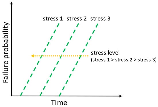
Figure 2.
Schematic illustration of the correlation of the stress level and failure probability.
Accelerated tests play an important role in the field of reliability by serving various purposes. They are employed in establishing a correlation between the operating conditions and product reliability and gain knowledge of the possible failure modes influencing the reliability under given operating stresses beforehand. The accelerated tests are also used in the identification of design failures and manufacturing defects and comparing the performances of the different designs, components, operating conditions, etc., thereby aiding in the determination and demonstration of reliability.
The different types of accelerations used in reliability testing can be classified as high usage rate, overstress testing, censoring and degradation [19]. In high usage rate, the components are operated at higher speeds or are operated for longer fractions of time than those in field operations, causing the increase in degradation rate. In overstress testing, the stresses such as thermal loads, mechanical loads, humidity, etc., in the test are at higher levels than those used in field conditions. The high usage rate and overstress tests can be run either until the component failure occurs, or the tests can be terminated before failures. When the tests are terminated before complete failure occurs, such accelerated tests are termed censored tests. Censoring is used for products with very high reliability where the information on early failures is required. In the case of degradation testing, instead of failures, the performance of the component is analyzed at different stages of test duration.
The data from the accelerated tests can be classified as life data or performance data [19]. The performance data are analyzed by fitting the degradation model to the data, and the relationship between the performance, stress and lifetime is predicted. In the case of performance data, the degradation paths are usually extrapolated using specific physical or statistical models, and the lifetime is predicted. The life data classification depends on the test conditions. The data from the tests where the failure of all the components is allowed to occur are called complete data [20]. In such data, the exact times to failure for all the components are known. In the case of censored tests, the data are known as censored data, which could be singly censored or multiply censored. Further, the censored data could be time-censored or failure-censored [20]. In the case of time-censored data, the tests are allowed to run until the fixed time and are independent of the number of failures. In time-censored data, the components could fail either completely, partially or not at all. In the case of failure-censored data, the tests are terminated after the predefined number of failures occur. In such cases, the length of test duration is not fixed. In multiply censored data, the components are put to the test at different start times, resulting in a mixture of time-censored and failure-censored data [20]. The test data could also be based on the test intervals at which the components are taken out from the test for inspection of failures and are put back to be tested after completion of the inspection. The data collected from the tests could also be classified based on the competing failure modes, where the failure of the components is caused by the different failure mechanisms even under the same test conditions.
The data obtained from the accelerated tests can be used for analyzing the causes of failures, as well as generating life expectancy models, in order to determine the reliability and remaining useful life of the component. An overview of the different types of modeling approaches for the determination of the remaining useful life in industries, along with their advantages and disadvantages, is given in [10]. The lifetime prognosis models are broadly classified into four main categories as knowledge-based models, life expectancy models, artificial neural networks and physical models. The knowledge-based models investigate the similarities between the observations from the present test and the data from previous similar tests and extrapolate the lifetime based on previous events. The life expectancy models estimate the lifetime by performance degradation, either through statistical or stochastic methods. The artificial neural networks predict the lifetime from the mathematical representation of the system, which in turn is established using the observation data. The physical models use the mathematical functions representing the physics of failure and degradation processes and are system-specific.
2.1. Acceleration Factor
In the case of electrical connectors, the majority of failures occur due to thermal and mechanical stresses [2,4]. The Norris–Landzberg model and Modified Norris–Landzberg model are used for the determination of the acceleration factor (AF).
2.1.1. Norris–Landzberg Model
The Norris–Landzberg model is a further improvement of the Arrhenius model [21,22,23] and Coffin–Manson [24,25,26,27] model. It combines both the models and, along with that, includes the influence of the thermal cycling frequency and maximum temperature. The acceleration factor is calculated as follows (Equation (1)) [24,25,26]:
where is the temperature difference in the test and field, is the coefficient of damage due to the temperature difference in thermal cycling, and are the thermal cycling frequencies in the field and test and is the damage coefficient due to the thermal cycling frequency. is the activation energy, is the Boltzmann constant and and are the maximum temperatures in the field and test. The values of range from 1.9 to 2 in various works. The value of is 1/3 [26,28,29,30].
2.1.2. Extended Norris–Landzberg Model
The extended Norris–Landzberg (ext. N-L) model is applicable to accelerated tests combining thermal and vibrational stress. It is an extension of the Norris–Landzberg model for an acceleration factor where the influence of the vibration loading is included. The acceleration factor based on the extended Norris–Landzberg model is given as follows (Equation (2)) [4]:
where and are the vibration load in accelerated test and field conditions, respectively, and is the coefficient of vibration.
2.2. Failure in Time (FIT) Rate
The mean time to failure (MTTF) can be obtained as a function of the failure probability with respect to time. In general practice, the time to failure data are modeled using the probability distributions, and the probability density function and instantaneous failure rates are determined. The normal, lognormal, exponential, Gaussian, Weibull and extreme value distributions are the most commonly used distributions for modeling the time to failure data [10,31]. The equations in the following section are established according to [19].
The failure rate can be written as the ratio of the number of failures to the cumulative operation time, also known as equivalent device hours (EDHs), and given as follows [32] (Equation (3)):
where is the total number of devices in the test, is the test duration in hours and is the acceleration factor. The acceleration factor is the time acceleration obtained by operating the components at higher stress levels and is used to convert the test duration in accelerated tests to the equivalent time in the field. The models for calculating the FIT rate are discussed further in this section.
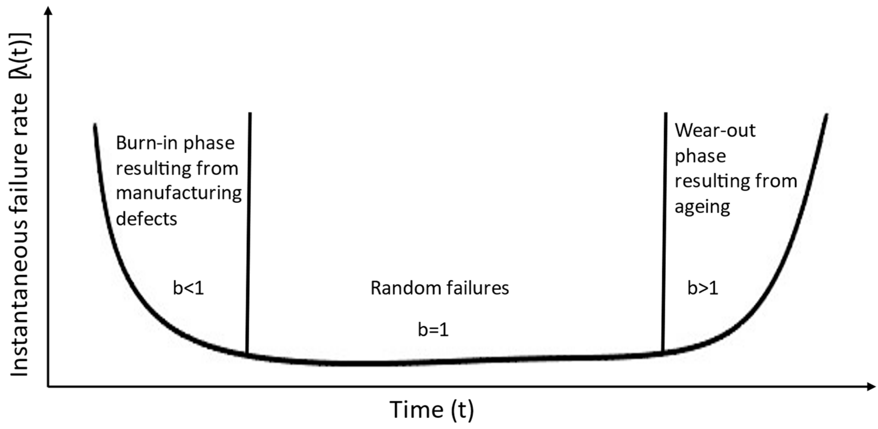
In a given component population, there exists a possibility of a set of components exhibiting a high failure rate in the initial phase of life, after which the failure rate stabilizes in the intermediate phase, and towards the end of life, the failure rate starts increasing rapidly. The failure rate in the initial phase is termed the “burn-in phase”, which could occur due to manufacturing defects. In the intermediate phase, the failures are randomly occurring, and the failure rate is almost constant. It is termed as the “useful life of the component”, which is important from a reliability point of view. In actual cases, the instant failure rate during the useful life could show a slightly upward trend. Towards the end phase of the life of a component, the failure rate shows a significant increase resulting from the wear-out of the components due to ageing. The combination of the failure rates in these three phases of the component’s life is represented by a bathtub curve, as shown in Figure 3. The life distributions followed by the component during these three phases are different. Such decreasing, constant and increasing failure rates are efficiently modeled using Weibull distribution. The Weibull shape parameter during the burn-in phase is less than 1, and in the useful life phase, it is equal to 1, while in the wear-out phase, it is greater than 1.
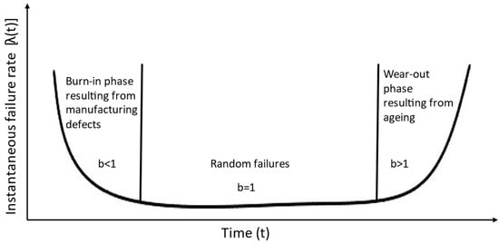
Figure 3.
The development of the shape parameter b over the lifetime as a so-called “bathtub curve” [19], graphically renewed.
The failure in time (FIT) rate is also one of the measures of the component’s reliability and is the measure of failure rates in one billion hours of operation, given as follows (Equation (4)):
It can be seen from the equation for the FIT rate that the determination of the failure rate forms the basis of the reliability estimation. The failure rate can be determined using different probability distributions, of which exponential, Weibull and Chi-square are commonly used for modeling.
The exponential distribution is used for modeling the constant failure rates. Based on the exponential distribution, the cumulative distribution function of the fraction of the components failing by the time is given as follows (Equation (5)):
where is the characteristic lifetime.
Also, the failure rate of the exponential distribution is given as follows (Equation (6)):
Thus, (Equation (7)) is
The Weibull distribution can model various types of failures, and because of this, it is the most widely used distribution in reliability estimation. Using the two-parameter Weibull distribution with a scale parameter and shape parameter , the cumulative distribution function of the fraction of components failing by time is given as follows (Equation (8)):
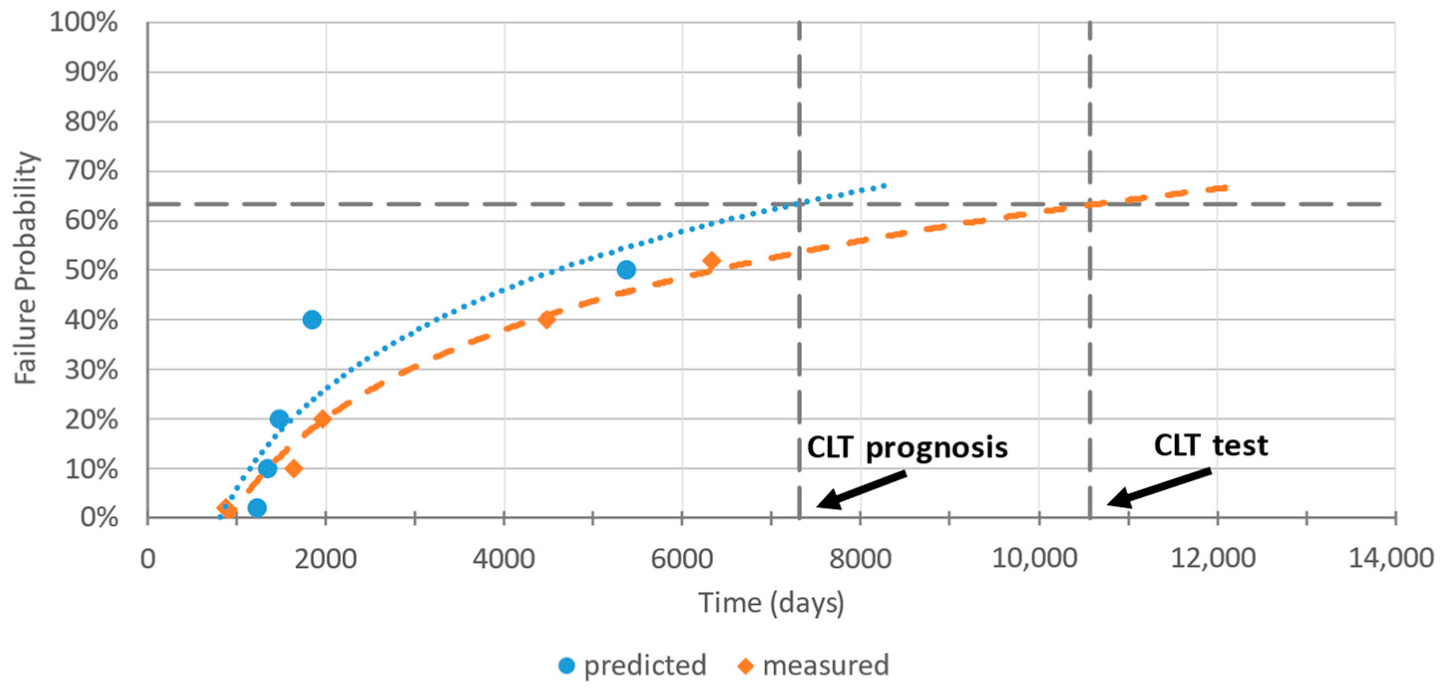
The scale parameter has the same unit as time, while the shape parameter represents the slope which can be estimated from the fitted Weibull plot. Also, all the curves, irrespective of the parameter value, intersect at the 63.2nd percentile. The scale parameter is thus called the characteristic lifetime (CLT). In other words, the CLT represents the time of occurrence of a 63.2% population failure. The CLT can be determined by modeling the time to the failure data using a Weibull distribution. In order to reliably determine the CLT, it is ideal to have at least 20% to 30% component failures during the test. The failure rate using the Weibull distribution is obtained as follows (Equation (9)):
As seen in Figure 3, the shape parameter for the constant failure rate is equal to 1. Therefore, for a constant failure rate, the Weibull failure rate becomes equal to the exponential failure rate and can be calculated as follows (Equation (10)):
The Chi-square distribution can be used for the estimation of the FIT rate when the failure rate follows the exponential distribution. The advantage of using a Chi-square distribution is that it can be used in cases where the number of failures during the test is very low or even equal to zero. The number of failures is obtained using the percentile values of the Chi-square distribution for the corresponding degrees of freedom (DOF) and confidence level using Equation (11):
where
Therefore, the failure rate using Equation (11) and Chi-square distribution is given as follows (Equation (12)):
As can be seen from Equation (12), the Chi-square distribution can be used to determine the failure rates even in the tests with no occurrences of failures until the end of the test duration. The FIT rate based on the Chi-square distribution is calculated as follows (Equation (13)):
3. Models for Prognosis of Reliability and Lifetime of Connectors
In cases where the failure mechanisms are known, physical models can be used to predict the connectors’ lifetime. One such example of physical models is the calculation model for the prediction of the wear of coatings of electrical connectors [33,34,35].
The applicability of a physics-based model depends on a comprehensive understanding of the damage mechanisms involved. Due to the complexity and variety of these mechanisms, as well as the possible interactions between different damage mechanisms in electrical connectors, this requirement is rarely fulfilled [36].
3.1. Statistical Model for State of Health (SoH) and Lifetime Prognosis
The electrical resistance is the most important performance parameter in electrical connectors. An electrical connector is said to have failed when its electrical resistance rises beyond the permissible limit, and hence, it is unable to conduct the required current or signal. Therefore, the lifetime, as well as extent of degradation and state of health, of an electrical connector can be monitored through the development of electrical resistance in the given connector [14,15]. In the case of electrical connectors, the lifetime is very long, making it almost practically impossible to gather failure data. Even at accelerated stress levels, the time required for an adequate number of failures to occur for reliable prognosis could be very long. In the case of connectors with very high reliabilities, there exists a possibility of no occurrence of failures even at accelerated stress levels. In order to estimate the lifetime in a short test duration, the electrical resistance development resulting from the given test or operation duration is extrapolated until the failure criteria through the remaining useful life estimation models. These models apply general statistics or machine leaning approaches for the prognosis. The statistical methods can be based on probability distributions [9,17,36] or distribution-free methods [15,36]. The similarity in all the approaches is the extrapolation of the degradation path, i.e., the development of the contact resistance in order to predict the time to failure. Also, through the state of health indicators, the state of health of electrical connectors can be monitored and predicted. The monitoring and forecasting of the state of health of electrical connectors can in turn assist in the prognosis and management of system health in critical and sophisticated systems.
The state of health indicators such as the surge point, time to surge, quotient q and prognosis of the time to failure for the given failure probability are defined in [36]. Also, the data-driven statistical procedure for the determination of characteristic lifetime (CLT) in order to determine the reliability using the FIT rate and Equation (10) is defined. The CLT determination applies a normal distribution, whereas in [36], the negatively skewed generalized extreme value distribution is used for CLT prognosis. Alternatively, the distribution-free method applying the percentiles of measured contact resistance instead of the standard variates of distribution can be used. The direct correlation between the electrical resistance development in the short term and long-term failure development forms the basis of the statistical procedure for estimating the CLT and FIT rate. Figure 4 shows the distribution of resistance values over the failure probabilities according to the standard normal distribution. The higher electrical resistance values represent the heavily degraded connectors. The given failure probability is equivalent to the corresponding percentage area under the distribution curve on the upper side. For, e.g., a contact resistance between 80% and 100%, i.e., the top 20% values correspond to the 20% contact population failure during the test or operation. The standard variates of the corresponding probability distribution and the failure probability, along with the mean and standard deviation of the electrical resistance, are then used to obtain the upper scatter of resistance, which is then used for extrapolation to determine the time to failure. In the distribution-free method, the actual percentiles of measured contact resistance are used to obtain the upper scatter and for extrapolation to predict the time to failure. For, e.g., the upper spread of electrical resistance, a 20% failure probability corresponds to the 80th percentile of the measured contact resistance. Through the proposed statistical procedures in [36], the time needed for a precise estimation of the reliability of electrical connectors subjected to thermal and mechanical loads is reduced by 85% to 98%, thereby saving considerable time and resources.
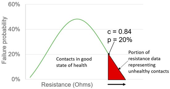
Figure 4.
Distribution of resistance values over failure probabilities according to standard normal distribution.
3.2. Electrical Contact Resistance and Failure Pattern Development
In order to investigate the development of contact resistance of the population of electrical connectors in a test, general statistical terms such as mean, standard deviation and standard variates of the normal distribution are used. The upper scatter of the electrical resistance for the corresponding probability distribution is given as follows (Equation (14)):
- —upper end of the spread of contact resistance at a given time t and failure probability p;
- —mean of contact resistance;
- —standard deviation;
- —standard variate score, estimated from the given distribution.
Originally, the standard normal distribution is used to obtain the c-scores for further analysis and for the results in the respective section.
For the exploratory data analysis, the upper spread of the contact resistance, , is calculated with a score of 2, i.e., a 4 level. However, the values of the scatter on the upper spread are considered for the analysis to understand the extent of degradation in the connector population. Thus, is given as follows (Equation (15)):
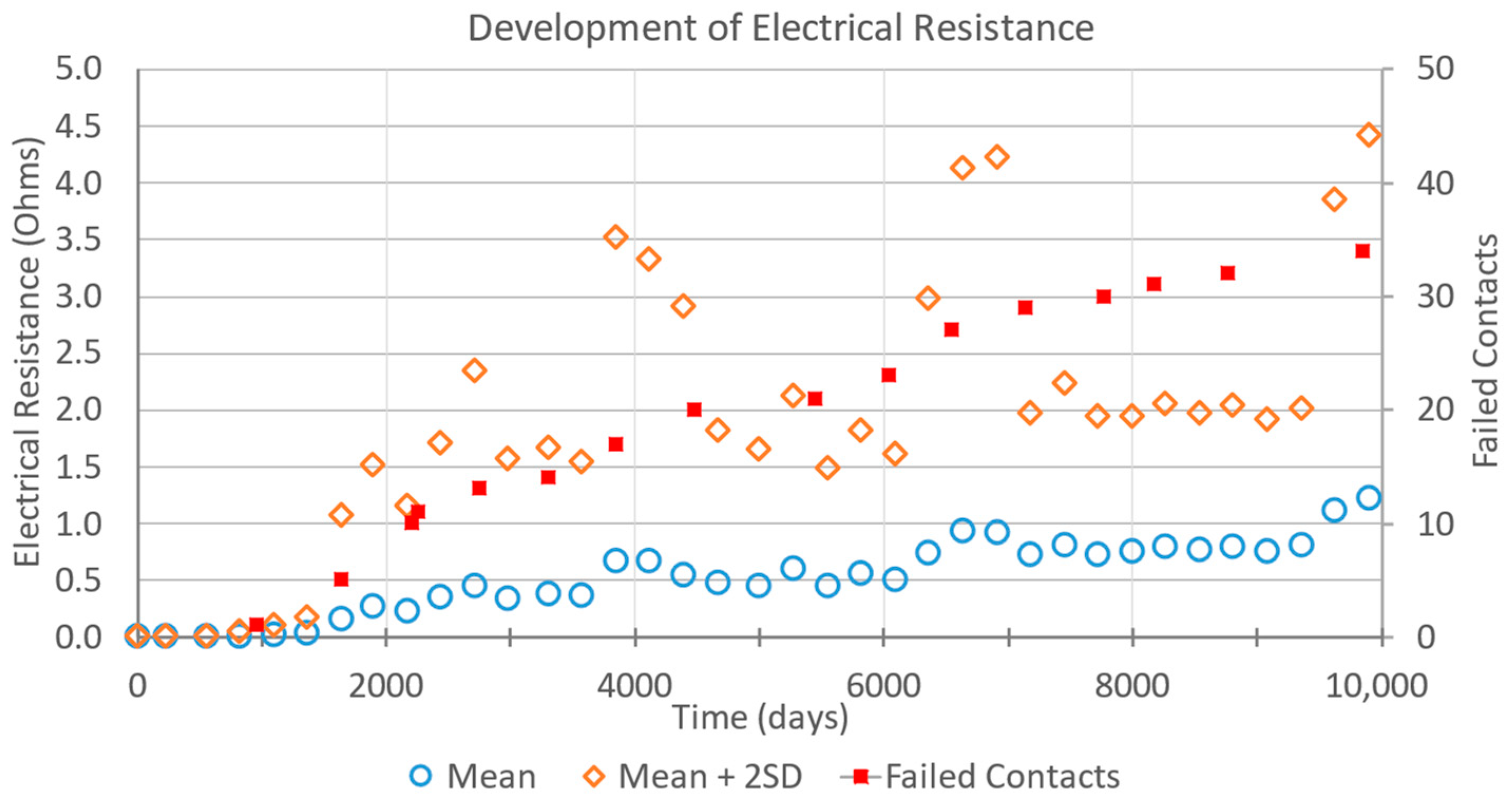
The electrical resistance of the connector remains stable in the beginning of the operation, as illustrated in Figure 5. During this phase, the standard deviation of the electrical resistance is also smaller. As time progresses further, the degradation caused by failure mechanisms such as stress relaxation and fretting wear and corrosion results in a gradual increase in the contact resistance. Also, the standard deviation of the resistance shows a noticeable increase. When one or more contacts in the given population approach failure, the mean and upper spread of the resistance show a sudden increase. This point of sudden increase in the mean and upper scatter of electrical resistance is termed the surge point, and the time to the occurrence of the surge point is termed the time to surge. In the majority of cases, it has been observed that the surge point is followed by the first failure. In Figure 5, the surge in the electrical resistance occurs around 800 days, and the first failure occurs after 950 days. The connectors with low reliability have a shorter time to surge, while those with intermediate reliability have a comparatively longer timer to surge. The electrical connectors with very high reliability and no failures possibly do not exhibit a surge in the upper spread of resistance.
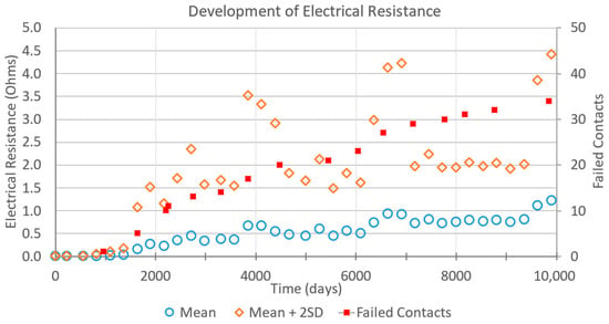
Figure 5.
Contact resistance development and connector failure.
3.3. Quotient q
The quotient is used to obtain an estimation of the degree of degradation that has occurred in the connector at a given point in time with respect to the initial electrical resistance. It is defined as the ratio of the upper spread of electrical resistance, , at the given time to the mean initial electrical resistance and calculated as follows (Equation (16)):
where means the initial electrical resistance.
The value of quotient provides an effective estimation of the possibility of the occurrence of the failures in the near future. Also, it is a reliable state of health indicator for the stability, i.e., the degree of fluctuation in the electrical resistance, of the connector. The advantage of quotient is that it can be determined at any given point in time based on the time to surge, which only occurs after reaching a certain amount of degradation. The very highly stable and reliable connectors have smaller values of quotient , which are generally below 2. Such connectors do not show failures during longer test durations. The connectors with > 4 are found to show one or more failures during their lifetime. The values at the surge for the majority of the electrical connectors’ designs lie between 4 and 50. The quotient is connector-specific and hence cannot be applied as a basis of comparison between different connectors.
3.4. Failure Time Prognosis
According to the FIT rate equation based on the Weibull function (Equation (10)), the characteristic lifetime (CLT), representing the time to 63.2% connector failures, is one of the required quantities for the determination of the failure in time (FIT) rate, with the acceleration factor being another required quantity. The acceleration factor can be calculated through the different acceleration factor models and is independent of the test duration. In standard practice, a time to failure data of 30% to 50% failures is recorded, and by fitting the Weibull distribution to the data, the characteristic lifetime is estimated and used for the FIT rate calculation. In actual accelerated tests, depending on the reliability of the connector, the time to 63.2% failures could be very long, whereas in some cases, even the minimum required failures for distribution fitting might not occur. Therefore, there is scope for the development of a statistical procedure to determine the CLT using short-term test data.
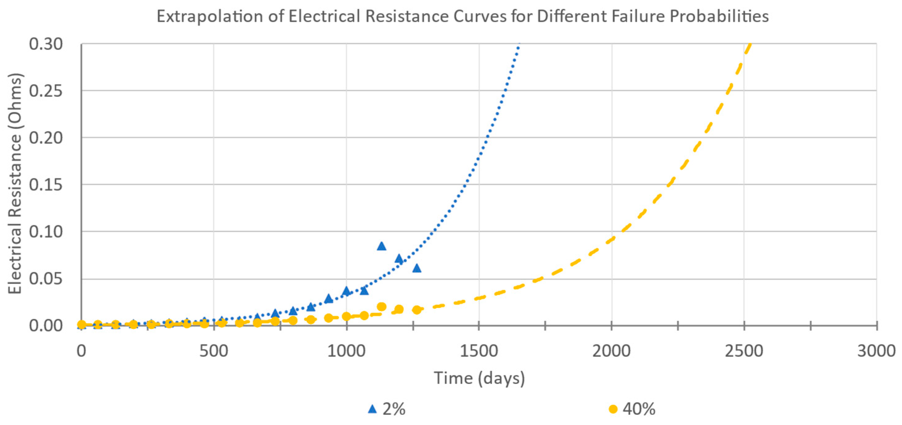
The surge point indicates the occurrence of the first failure in the test. The contact resistance data until the surge point are used for the prognosis of the time to failure of the given failure probability through an extrapolation of the degradation path, represented by the upper scatter (Equation (14)). The -scores of the standard normal distribution and negatively skewed generalized extreme value distribution are used for calculating the upper scatter for the respective failure probabilities [36] and are given in Table 1. The upper scatter of electrical resistance is calculated for the 2%, 10%, 20% and 40% failure probabilities with the contact resistance data until the surge point. The data are then exponentially extrapolated to obtain the time to failure for corresponding failure probabilities (Figure 6).

Table 1.
The c-score for normal and GEV distribution of different failure probabilities.
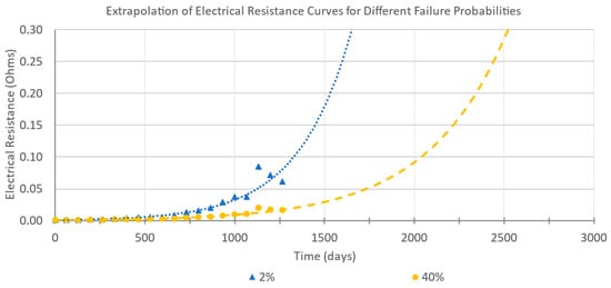
Figure 6.
Exemplary exponential extrapolation (dotted lines) of the data for different failure probabilities.
The exponential function fitted to the data is given as follows (Equation (17)):
where is the time to failure for a given failure probability . The coefficients and are obtained from the exponential fit. The extrapolated curves for different failure probabilities are shown in Figure 6. The higher the number of failures is, the longer it takes for the extrapolation to reach the resistance threshold of 300 mΩ.
The time to failure for a given failure probability is calculated by substituting with the value of electrical resistance corresponding to the failure criteria as follows (Equation (18)):
The predicted time to failure data of 2%, 10%, 20% and 40% failure probabilities are plotted and extrapolated until the 63.2% failure probability in order to obtain the CLT (Figure 7). The extrapolation of the time to failure data in the case of the distribution-based method is carried out via logarithmic fitting.

Figure 7.
Measured and predicted failure times plotted over their respective failure probabilities (circular and diamond pointers) with logarithmic extrapolation (blue and orange dotted curves) till 63.2% failure probability to get CLT.
3.5. Experimental Testing
For the validation of the proposed approach to determine the state of health and lifetime of electrical connectors, the data of more than 20 different connector types with approximately 4000 contacts and more than 80 lifetime tests with different acceleration levels were analyzed.
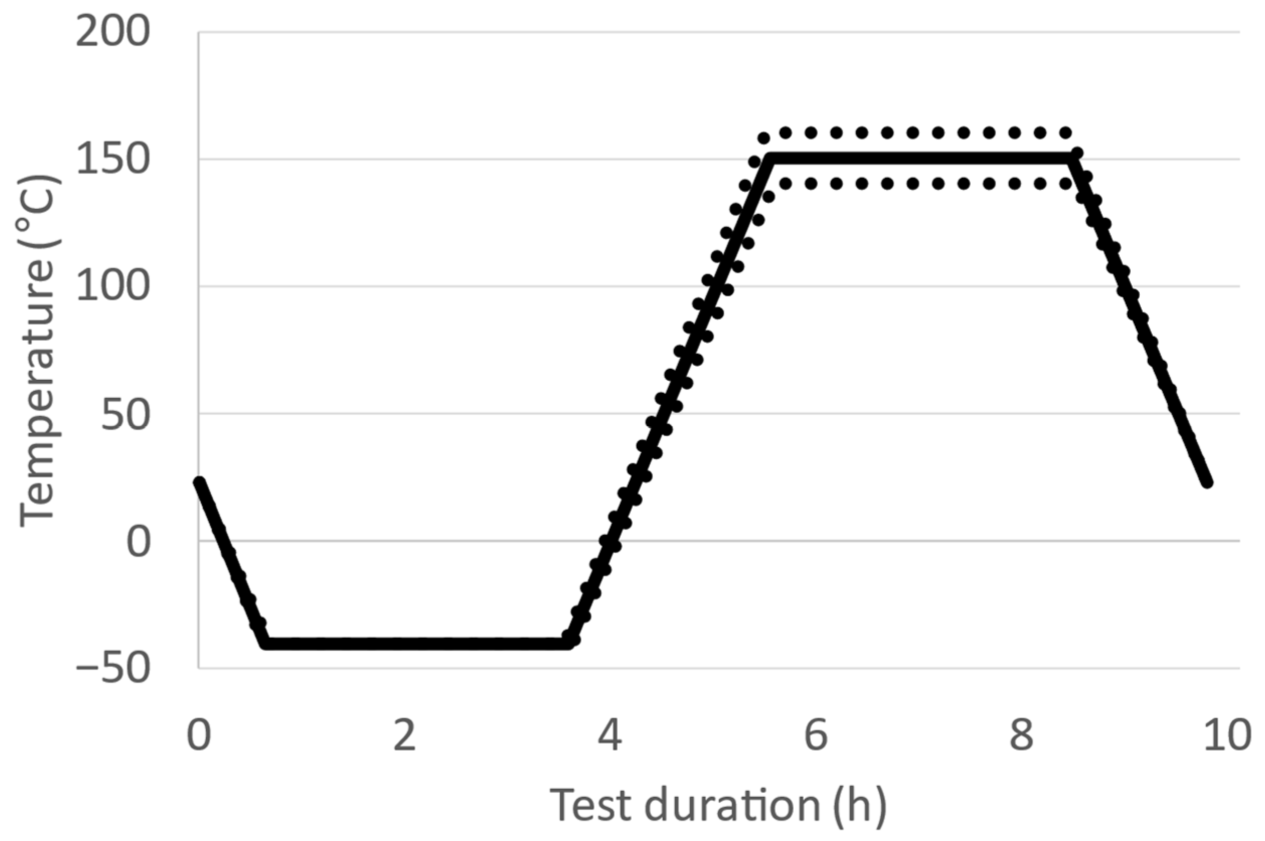
The lifetime tests were carried out using thermal cycling tests with a cycle duration of 10 h in accordance with [37]. As shown in Figure 8, the lower temperature of −40 °C and upper temperature of 140–160 °C are held constant for 3 h each. In the phases between the temperature limits, the temperature gradually increases/decreases over a duration of 2 h. About 50 contacts of one connector type are placed in the temperature chamber (Vötsch VTS 7021-5, Weiss Technik GmbH, Reiskirchen, Germany) at the same time (Figure 9).

Figure 8.
Schematic representation of the temperature profile during the thermal cycling test.
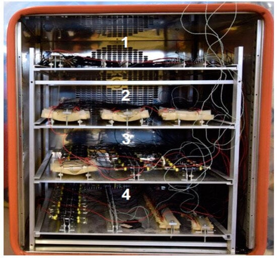
Figure 9.
Illustration of the connectors placed in the four levels of the temperature chamber.
The resistance values were measured using a Keithley (Keithley Instruments, Solon, OH, USA) 3706 A System Switch/Multimeter with a constant current of 100 mA. For each cycle, three independent measurements were taken for every single contact about 2 h after reaching the upper temperature limit. A schematic illustration of the resistance measurement is shown in Figure 10. L1 to L6 represent the female connector parts and M1 to M6 the male counterparts.

Figure 10.
Schematic representation of the resistance measurement to ensure a constant current during the measurement.
The current flows from contact 1 to contact 2 and so on. This way, it is ensured that the voltage values are measured with the same current for all 50 contacts. In case of an occurring failure, the respective contact is bypassed.
In this way, the proposed approach is applicable to the wide variety of electrical connectors, irrespective of their design and operating conditions. In order to illustrate the effectiveness of the approach, the prognosis results corresponding to one connector each from the categories unstable (Connector A) and stable (Connector B) are illustrated, and the respective predicted characteristic lifetimes are compared with the measured values. It should be noted that the stable connectors are the ones exhibiting a larger reliability in comparison to the unstable connectors. Since the tests have been performed with different acceleration factors, the results are converted to the comparable operating stresses. All evaluations in this section have been performed using the standard normal distribution.
4. Results
The failure pattern and electrical resistance development in connector A and connector B are highlighted in Figure 11. A total of 29 failures are recorded after 6200 days of operation in connector A, whereas in the case of connector B, 8 failures are recorded after 10,500 days of operation. Initially, the contact resistance in both the connectors is stable, with mean and upper spread values coinciding with each other. With increasing degradation, the standard deviation of the contact resistance increases, and a sudden increase in the contact resistance is observed near the surge point. The surge point is usually succeeded by the first failure in the majority of cases. The surge in connector A and connector B, as indicated by the upper spread of contact resistance, occurs around 1000 days and 4000 days of operation, respectively.

Figure 11.
Development of mean resistance value, as well as upper spread and number of failed contacts, of connector types A (left) and B (right).
The measured characteristic lifetimes are determined via a Weibull plot based on the actual failures that occurred during the tests. The detailed procedure to determine the characteristic lifetime based on Weibull plots is given in [20]. The predicted characteristic lifetimes based on the extrapolation of the times to failure of various failure probabilities, as described in the section titled “Failure Time Prognosis” are highlighted in Table 2. Additionally, the q values at the time of evaluation, i.e., surge, are given.

Table 2.
Results of characteristic lifetimes of two exemplary electrical connectors.
Based on the measured characteristic lifetime, it can be seen that connector A has a lower stability than connector B. Connectors A and B have a measured characteristic lifetime of 12,300 days and 105,000 days, respectively (Table 2). The surge in electrical resistance in connector A occurs after 1000 days (Figure 11, left), whereas in connector B, the surge is observed after 4000 days (Figure 11, right). The q value at the surge in connectors A and B is 25 and 40, respectively. Thus, the q value which gives the extent of degradation at a given time is unique to a connector type and should not be used as a basis of comparison between different connector types.
The predicted characteristic lifetime of connector A is 8000 days, which is 35% lower than the measured value. On the other hand, the predicted characteristic lifetime of connector B is 79,500 days, which is approximately 24% lower than the measured value. Given the randomness in the failures and lifetimes of the electrical connectors, the predicted characteristic lifetime can be considered to be adequately precise and can be reliably used for the determination of the FIT rate values. Therefore, the test duration required for reliable prediction of the characteristic lifetime in connector A and connector B is reduced by 91% and 96%, respectively.
Apart from the standard normal distribution, the negatively skewed generalized extreme value (GEV) distribution, as well as a distribution-free method based on the percentiles of measured electrical resistance, can be effectively employed for the prognosis of the characteristic lifetime. When compared with the measured characteristic lifetime, the prognoses derived from the GEV distribution and percentiles of electrical resistance are observed to obtain better estimates of the characteristic lifetime in comparison to the standard normal distribution. However, the advantage of using a standard normal distribution is that the predicted reliability is on the conservative side and hence produces estimations that are on the safer side. The proposed approach can also be applied for the estimation of the characteristic lifetime in case of the connectors showing no failures. In this way, the need to conduct very long accelerated tests for the determination of the reliability of electrical connectors is eliminated with the proposed approach.
5. Conclusions
The knowledge about the operating stresses and failure mechanisms of electrical connectors is an important basis for designing lifetime tests. Modern electrical connectors have very high reliability. Due to the large number of electrical connectors used in vehicles and their associated relevance for the vehicle’s reliability, the determination of connectors’ reliability is still an important issue. A data-driven approach was introduced for the prediction of the reliability of electrical connectors with data from the early phase of accelerated tests. These data can be used for relatively precise predictions of the lifetime of electrical connectors and also enable a distinction of connectors with respect to their performance stability and reliability. The data-driven approach is validated by comparing the predicted characteristic lifetimes with the lifetime obtained from long-term accelerated tests. With this statistical method, the lifetime of electrical connectors can be reliably estimated, irrespective of the stress levels and the occurrence of a number of failures.
The lifetime predictions using the single-term exponential function have good precision (Equation (17) and Figure 6) and can therefore reliably be applied for health monitoring and diagnostics of a connector and, in turn, physical network’s health. The remaining useful life of electrical connectors can be obtained in real time, and preventive measures can be taken in case of upcoming failures.
Author Contributions
Conceptualization, J.S.; Methodology, J.S.; Formal analysis, A.S.; Investigation, A.S.; Resources, J.S.; Writing—original draft, A.S.; Writing—review & editing, J.S. and R.P.; Funding acquisition, J.S. All authors have read and agreed to the published version of the manuscript.
Funding
This study is financed by the German Federal Ministry for Economic Affairs and Climate Action (BMWK, IGF, 23011 N).
Data Availability Statement
The original contributions presented in the study are included in the article, further inquiries can be directed to the corresponding author.
Conflicts of Interest
The authors declare no conflicts of interest.
References
- International Organization for Standardization. Road Vehicles—Functional Safety—Part 5: Product Development at the Hardware Level, Genf; International Organization for Standardization: Geneva, Switzerland, 2016. [Google Scholar]
- Hilmert, D.; Yuan, H.; Song, J. The Analysis of Failure Mechanisms of Electrical Connectors in Long-term Use Field Vehicles. In Proceedings of the 2022 IEEE 67th Holm Conference on Electrical Contacts, Tampa, FL, USA, 23–26 October 2022; pp. 9–16. [Google Scholar]
- Callen, B.W.; Johnson, B.; King, P.; Timsit, R.S.; Abbott, W.H. Environmental degradation of utility power connectors in a harsh environment. IEEE Trans. Compon. Packag. Technol. 2000, 23, 261–270. [Google Scholar] [CrossRef]
- Song, J.; Yuan, H.; Koch, C. Accelerated Testing of Electromechanical Connectors Considering Thermal and Mechanical Loads. In Proceedings of the 2018 IEEE 64th Holm Conference on Electrical Contacts, Albuquerque, NM, USA, 14–18 October 2018; pp. 467–474. [Google Scholar]
- Kyeong, S.; Pecht, M.G. Electrical Connectors: Design, Manufacture, Test, and Selection; John Wiley & Sons: Hoboken, NJ, USA, 2020. [Google Scholar]
- Bock, E.M.; Whitley, J.H. Fretting corrosion in electrical contacts. In Proceedings of the 20th Annual Holm Seminar on Electrical Contacts, Harrisburg, PA, USA, 29–31 October 1974. [Google Scholar]
- Liu, H.; McBride, J.W. A Finite-Element-Based Contact Resistance Model for Rough Surfaces: Applied to a Bilayered Au/MWCNT Composite. IEEE Trans. Compon. Packag. Manuf. Technol. 2018, 8, 919–926. [Google Scholar] [CrossRef]
- Yuan, H.; Song, J.; Schinow, V. Fretting corrosion of tin coated electrical contacts: The influence of normal force, coating thickness and geometry of sample configuration. In Proceedings of the 2016 IEEE 62nd Holm Conference on Electrical Contacts, Clearwater Beach, FL, USA, 9–12 October 2016. [Google Scholar]
- Sun, B.; Yu, L.; Wang, Z.; Ren, Y.; Feng, Q.; Yang, D.; Lu, M.; Chen, X. Remaining useful life prediction of aviation circular electrical connectors using vibration-induced physical model and particle filtering method. Microelectron. Reliab. 2019, 92, 114–122. [Google Scholar] [CrossRef]
- Sikorska, J.Z.; Hodkiewicz, M.; Ma, L. Prognostic modelling options for remaining useful life estimation by industry. Mech. Syst. Signal Process. 2011, 25, 1803–1836. [Google Scholar] [CrossRef]
- Seehase, H. A reliability model for connector contacts. IEEE Trans. Reliab. 1991, 40, 513–523. [Google Scholar] [CrossRef]
- Pecht, M.G.; Jaai, R. A prognostics and health management roadmap for information and electronics-rich systems. Microelectron. Reliab. 2010, 50, 317–323. [Google Scholar] [CrossRef]
- Bierwirth, F.; Froeschl, J.; Gebert, J.; Herzog, H.-G. Determining Vehicle Energy Paths’ Remaining Useful Life using Design of Experiments. In Proceedings of the 2020 Fifteenth International Conference on Ecological Vehicles and Renewable Energies (EVER), Monte-Carlo, Monaco, 10–12 September 2020. [Google Scholar]
- Gómez-Pau, Á.; Riba, J.-R.; Moreno-Eguilaz, M. Time Series RUL Estimation of Medium Voltage Connectors to Ease Predictive Maintenance Plans. Appl. Sci. 2020, 10, 9041. [Google Scholar] [CrossRef]
- Martínez, J.; Riba, J.-R.; Moreno-Eguilaz, M. State of Health Prediction of Power Connectors by Analyzing the Degradation Trajectory of the Electrical Resistance. Electronics 2021, 10, 1409. [Google Scholar] [CrossRef]
- Zhao, Y.; Zio, E.; Fu, G. Remaining storage life prediction for an electromagnetic relay by a particle filtering-based method. Microelectron. Reliab. 2017, 79, 221–230. [Google Scholar] [CrossRef]
- Ren, Y.; Feng, Q.; Ye, T.; Sun, B. A Novel Model of Reliability Assessment for Circular Electrical Connectors. IEEE Trans. Components, Packag. Manuf. Technol. 2015, 5, 755–761. [Google Scholar] [CrossRef]
- Yu, Z.; Ren, Z.; Tao, J.; Chen, X. Accelerated Testing with Multiple Failure Modes under Several Temperature Conditions. Math. Probl. Eng. 2014, 2014, 839042. [Google Scholar] [CrossRef]
- Nelson, W.B. Accelerated Testing: Statistical Models, Test Plans and Data Analysis, 2nd ed.; John Wiley & Sons, Inc.: Hoboken, NJ, USA, 2004. [Google Scholar]
- Härtler, G. Das Lebensdauernetz—Leitfaden zur grafischen Bestimmung von Zuverlässigkeitskenngrößen der Weibull-Verteilung; Deutsche Gesellschaft für Qualität e. V: Frankfurt am Main, Germany, 1995. [Google Scholar]
- Klinger, D.J. On the notion of activation energy in reliability: Arrhenius, Eyring, and thermodynamics. In Annual Reliability and Maintainability Symposium. 1991 Proceedings; IEEE: New York, NY, USA, 1991; pp. 295–300. [Google Scholar]
- Bayle, F.; Mettas, A. Temperature acceleration models in reliability predictions: Justification & improvements. In Proceedings of the 2010 Proceedings—Annual Reliability and Maintainability Symposium (RAMS), San Jose, CA, USA, 25–28 January 2010; pp. 1–6. [Google Scholar]
- Ostendorf, F.; Wielsch, T.; Reiniger, M. Reliability assessment and field failure predictions—A prognostic model for separable electrical contacts. In Proceedings of the ICEC 2014; The 27th International Conference on Electrical Contacts, Dresden, Germany, 22–26 June 2014; pp. 1–6. [Google Scholar]
- Vasudevan, V.; Fan, X. An acceleration model for lead-free (SAC) solder joint reliability under thermal cycling. In Proceedings of the 2008 58th Electronic Components and Technology Conference, Lake Buena Vista, FL, USA, 27–30 May 2008; pp. 139–145. [Google Scholar]
- Dauksher, W. A Second-Level SAC Solder-Joint Fatigue-Life Prediction Methodology. IEEE Trans. Device Mater. Reliab. 2008, 8, 168–173. [Google Scholar] [CrossRef]
- Spahr, M.; Kreitlein, S.; Haas, R.; Jaumann, A.; Gläßel, T.; Spreng, S.; Franke, J. Application and comparison of analytic accelerated test-models for lifetime prediction of a novel contacting method. In Proceedings of the 2016 IEEE 62nd Holm Conference on Electrical Contacts, Clearwater Beach, FL, USA, 9–12 October 2016; pp. 94–99. [Google Scholar]
- Ciappa, M.; Carbognani, F.; Fichtner, W. Lifetime prediction and design of reliability tests for high-power devices in automotive applications. IEEE Trans. Device Mater. Reliab. 2003, 3, 191–196. [Google Scholar] [CrossRef]
- Norris, K.C.; Landzberg, A.H. Reliability of Controlled Collapse Interconnections. IBM J. Res. Dev. 1969, 13, 266–271. [Google Scholar] [CrossRef]
- Eckel, J.F. The influence of frequency on the repeated bending life of acid lead. Proc. Am. Soc. Test. Mater. 1951, 51, 745–760. [Google Scholar]
- Gohn, G.R.; Ellis, W.C. The fatigue test as applied to lead cable sheath. Proc. ASTM 1951, 51, 721–744. [Google Scholar]
- Rausand, M.; Høyland, A. System Reliability Theory—Models, Statistical Methods, and Applications, 2nd ed.; John Wiley & Sons, Inc.: Hoboken, NJ, USA, 2004. [Google Scholar]
- Ellerman, P. Calculating Reliability Using FIT & MTTF: Arrhenius HTOL Model [Internet]. Available online: https://www.google.com.hk/url?sa=t&source=web&rct=j&opi=89978449&url=https://www.microsemi.com/document-portal/doc_view/124041-calculating-reliability-using-fit-mttf-arrhenius-htol-model&ved=2ahUKEwi2p5PZ6piHAxVUh68BHSuGBFUQFnoECBsQAQ&usg=AOvVaw1i8HeKszUQig5FSVQ2CYL5 (accessed on 22 May 2023).
- Song, J.; Schinow, V.; Yuan, H. Third bodies in electrical contacts—Wear and electrical performance. In Proceedings of the 2017 IEEE 63rd Holm Conference on Electrical Contacts, Denver, CO, USA, 10–13 September 2017; pp. 117–124. [Google Scholar]
- Yuan, H.; Song, J.; Schinow, V. Simulation methodology for prediction of the wear on silver-coated electrical contacts with a sphere/flat configuration. IEEE Trans. Compon. Packag. Manuf. Technol. 2018, 8, 364–374. [Google Scholar] [CrossRef]
- Yuan, H.; Song, J.; Schinow, V. Modification of the Calculation Model for the Prediction of the Wear of Silver-Coated Electrical Contacts with Consideration of Third Bodies. In Proceedings of the 2018 IEEE 64th Holm Conference on Electrical Contacts, Albuquerque, NM, USA, 14–18 October 2018; pp. 310–316. [Google Scholar]
- Song, J.; Shukla, A.; Probst, R. Prediction of failure in time (FIT) of electrical connectors with short term tests. Microelectron. Reliab. 2022, 138, 114684. [Google Scholar] [CrossRef]
- DIN EN 60068-2-14*VDE 0468-2-14; Environmental Testing—Part 2-14: Tests—Test N: Change of Temperature (IEC 60068-2-14:2009); German Version EN 60068-2-14:2009. VDE-VERLAG GmbH: Berlin, Germany, 2010.
Disclaimer/Publisher’s Note: The statements, opinions and data contained in all publications are solely those of the individual author(s) and contributor(s) and not of MDPI and/or the editor(s). MDPI and/or the editor(s) disclaim responsibility for any injury to people or property resulting from any ideas, methods, instructions or products referred to in the content. |
© 2024 by the authors. Licensee MDPI, Basel, Switzerland. This article is an open access article distributed under the terms and conditions of the Creative Commons Attribution (CC BY) license (https://creativecommons.org/licenses/by/4.0/).

